i F p L ! 'Cl-FT! O IN! V /jt.\. . - i .7 ^ i V-/ «
Economics
_■ V:. ,_i i. M jn>l V O tt. W *15^ i;»4^Ju ly 20C3
/ f C 7 9 a s “ u S 9 IL O O OA POWERFUL TEST FOR UNIT ROOT
AND AN APPLICATION TO GNP OF SEVEN OECD COUNTRIES
The Institute o f Economics and Social Sciences
of
BiUcent University
by
ALÎYE ÜSTÜNDAG
In Partial Fulfillment of the Requirements for the Degree of
MASTER OF ARTS IN ECONOMIC
m
THE DEPARTMENT OF
ECONOMICS
BiLKENT UNIVERSITY
ANKARA
July 2000
" IL·
Z O O О
I certify that I have read this thesis and that in my opinion it is fully adequate, in scope and in quality, as a thesis for the degree of Master of Arts.
Asst. Prof. Dr. Mehmet Caner (Supervisor)
I certify that I have read this thesis and that in my opinion it is fully adequate, in scope and in quality, as a thesis for the degree o f M aster o f Arts.
Asst. Prof. Dr. Erdem Başçı
I certify that I have read this thesis and that in my opinion it is fiilly adequate, in scope and in quality, as a thesis for the degree of M aster o f Arts.
Asst. Prof. Dr. Hakan Berument
Approved for the Institute of Economics and Social Sciences:
ABSTRACT
A POWERFUL TEST FO R UNIT ROOT
AND AN APPLICATION TO GNP OF SEVEN OECD COUNTRIES
Aliye Ustiindag M.A. in Economics
Supervisor: Asst. Prof. Dr. M ehmet Caner July 2000
This thesis uses a powerful test, Dickey-Fuller Generalized Least Squares (DF-GLS), to see whether unit root exists or not in real GNP of OECD Countries - Australia, Canada, Germany, Japan, Italy, U.K. and U.S. - for the years between the first quarter o f 1960 and the second quarter of 1998 by using quarterly data that takes 1995 as base year. For this purpose a simple model with a deterministic component plus an error term, which is assumed to be AR (1), is used. The results of the regressions show the existence of unit root for all of the considered countries. Furthermore, we give flnite sample performances o f Augmented Dickey-Fuller (ADF) test and DF-GLS tests which Elliott et al. (1996) conducted by using Monte Carlo experiment.
K epvords: Unit root, DF-GLS, deterministic component, AR (1), ADF and
M onte Carlo experiment.
ÖZET
BİRİM K Ö K İÇİN GÜÇLÜ BİR TEST
VE BU TESTİN YEDİ OECD ÜLKESİNİN GSMH’SEVA UYGULAMASI
Aliye Üstündağ
İktisat Bölümü, Yüksek Lisans
Tez Yöneticisi: Yrd. Doç. Dr. Mehmet Caner Temmuz 2000
Bu tez güçlü bir test kullanarak - Dickey-Fuller Genelleştirilmiş Küçük Kökler
(DF-GLS) yedi OECD ülkelesinin - Avustralya, Almanya, Kanada, Japonya,
İngiltere, İtalya ve ABD - reel GSMH’sında 1960’ın ilk çeyreği ve 1998’in ikinci çeyreği arasında kalan dönem için (1995 yılını esas alarak) birim kökün olup olmadığına bakar. Bu amaçla deterministle kısım ve hata teriminin toplamından oluşan ve hata terimi AR(1) olarak kabul edilen basit bir model kullanılmıştır. Regresyon sonuçları adı geçen bütün ülkelerde birim kökün varlığını göstermektedir. Ayrıca, Elliott ve diğerlerinin (1996) yapmış olduğu Monte Carlo deneyini kullanarak, geliştirilmiş Dickey-Fuller (ADF) ve DF- GLS testlerinin sonlu örnek performanları verilmiştir.
A nahtar Sözcükler: Birim kök, DF-GLS, deterministik kısım, AR(1), ADF,
Monte Carlo deneyi
ACKNOWLEDGEMENTS
I would like to express my gratitute to Assistant Professor Dr. Mehmet Caner for drawing my attention to the subject, for providing me the necessary background that I needed to complete this study and the valuable supervision he provided.
I also would like to thank Assistant Professor Dr. Erdem Başçı, Professor Dr. Erinç Yeldan, Assistant Professor Dr. Hakan Berument, Assistant Professor Dr. Kıvılcım Metin Özcan and Assistant Professor Dr. Serdar Sayan for the understanding, patience and moral support they provided during my M.A. in Economics.
I am grateful to my family for the understanding, patience, moral and material support they provided during my whole education. Furthermore, I think it would be great ungratefulness not to recognize my sister Aylin’s supports. I think it would have been great unfairness to forget to thank for the moral support provided by Arzdar K raci. Finally, I thank to Gülşen Yılmaztürk, Mesut Açıkkol, Pınar Asöcal and Rezzan Aydmoğlu for their endless support.
Contents
1 Introduction
2 Theoretical Background
2.1 Asymptotic Properties o f a First-Order Autoregression When The True Coefficient is Less Than Unity in Absolute Value 2.2 Asymptotic Properties of a First-Order Autoregression
When The True Coefficient is Unity 7 2.3 The Data Generating Process 9 2.3.1 The Dickey Fuller Family of Unit Root Tests 10
3 The Data and Results 13
3.1 Finite Sample Performance 15
4 Conclusion 18 Select Bibliography 19 Appendix 20 A Data 21 B Figures 28 C Program 32 VI
LIST OF TABLES
Table I Table n Table i n Table IV
Critical Values for Linear Trend 13
Calculated Values for Linear Trend 14 Calculated Values for Linear Trend 14 Size and Size-Adjusted Power of Selected Tests 17 of The 1(1) Null; Mcnte Carlo Results 5% Level
LIST OF FIGURES
Figure B .l. Real GNP o f Australia 28
Figure B.2. Real GNP o f Canada 28
Figure B.3. Real GNP o f Germany . 29
Figure B.4. Real GNP o f Italy 29
Figure B.5. Real GNP o f Japan 30
Figure B.6. Real GNP o f U. K. 30
C h a p te r 1
Introduction
The recent method employed by Elliott, Rothenberg and Stock (1996) for an autoregressive unit root, for testing whether a univariate time series is integrated o f order one (difference stationary) against the hypothesis that it is integrated o f order zero (trend stationary), opened a new debate in economic literature.
Interest in this field starts with the seminal works o f Fuller (1976) and Dickey and Fuller (1979). They employed three types o f tests and their test statistics to determine whether a series contains a unit root, unit root plus drift;, and/(or) unit root plus drift plus a time trend under the assumption that the errors are statistically independent and uncorrelated. After Dickey and Fuller, Philips and Perron (1988) developed an extension o f Dickey and Fuller's testing procedure under the assumption that the residuals o f a unit root process are heteregenous and weakly dependent.
Although various testing principles developed in econometric literature, numerical calculations showed that power functions for these tests differ substantially and no general optimality theory have been developed in this field. Cheung and Chinn (1996) stressed that
Recently, concern has arisen regarding the low power o f conventional unit root tests, such as augmented Dickey-Fuller (ADF) test, and consequently, the apparent finding o f a unit root in GNP data using these tests. For
instance, Christiano and Eichenbaum (1990), Stock (1991), Rudebusch (1992, 1993), and Dejong, Nankervis, Savin, and Whiteman (1992) show that the ADF test has low power to differentiate between the trend and difference stationary properties o f G N P... *
Furthermore, Caner and Killian (2000) examine whether real exchange rates are mean-reverting or not. They emphasized that the standard tests o f unit root null hypothesis have not been able to provide guidance to economic theorists due to low power.^
However, the testing principle employed by Elliott et al. (1996) provides the locally most powerful test for testing whether the series is integrated o f order one or integrated o f order zero. DF-GLS test employed by Elliot et al. (1996) have higher- size adjusted power than the standard ADF test for almost all o f the data generating processes.
Cheung and Chinn (1996) used Dickey- Fuller generalised least squares (DF- GLS) technique to study the persistence o f U.S. GNP. They point out that the DF- GLS test o f Elliott et al. (1996) is more powerful than the original ADF test and approximately uniformly most power invariant.
Cheung and Lai (1998) again used DF-GLS test to examine the validity o f parity reversion in real exchange rates during the post-Bretton Woods period. As Cheung and Chinn (1996), they indicated that:
’ Cheung and Chinn (1996), page 1. ^ Caner and Kilian (2000), pages 1-2. ^ Cheimg and Chinn (1996), page 1.
In studying the asymptotic power envelope for various unit root tests, Elliott et al. (1996) propose a simple modification o f the augmented Dickey-Fuller (ADF) test such that the modified test can nearly achieve the power envelope using generalized least squares (GLS) estimation. The resulted DF-GLS test is shown to be approximately uniformly most powerful. Monte Carlo results confirm that the power improvement fi"om using the DF-GLS test can be large relative to standard ADF test."*
Basically, there are two main differences between the testing procedure o f Elliott et al. (1996) and Dickey and Fuller. Firstly, Elliott et al. (1996) assumes that errors are correlated and makes a transformation to make residuals o f the unit root process uncorralated. Secondly, Elliott et al. (1996) use GLS technique whereas others use least squares (LS) technique.
In the thesis, we employ the procedure o f Elliott et al. (1996) by using real GNP o f seven OECD countries; Australia, Canada, Germany, Italy, Japan, U.K. and U.S. by using seasonally unadjusted data - which took 1995 as base year- for the years between the first quarter o f 1960 and second quarter o f 1998.
We assume that the data y i.. .yx were generated as
yt = u t+ d t
ut = aut-i+Vt (t= l..,T )
(
1
.1
)(
1
.
2
)
Where dt and v, are deterministic trend and unobserved zero-mean error process, respectively. As usual, our interest is in the null hypothesis a = l (which implies the yt are integrated o f order one) versus |a |< l (which implies the yt are integrated o f order zero).
The organization o f the thesis is as follows: Chapter 2 provides a theoretical background in this field and presents the data generation process employed for testing process. Chapter 3 introduces and provides a comparison o f the finite sample performance o f usual Dickey-Fuller test and the test employed by Elliott et al. (1996). Finally, Chapter 4 provides the concluding remarks.
C h a p te r 2
Theoretical Background
2.1 Asymptotic Properties of a First-Order Autoregression When
The True Coefficient is Less Than Unity in Absolute Value
If a univariate process contains a unit root, asymptotic distributions and rates of convergence for the estimated coefficients of unit root processes differ from those for stationary process/
To see distributional properties of a stationary process, consider LS estimation o f a Gaussian AR (1) process.
yt = ayt-i+ vt (b=l,...,T)
(
2
.
1
)
where Vt is i.i.d. N(0, cr^), and initial value o f y is 0. The LS estimate o f a is given by
j l y t - i y .
a , =t /=1T
(
2
.
2
)
f=l
if |a |< l, then
r '" (d r -a )-> A i(0 ,(l-o '))
(2.3)Equation 2.3 is also valid when a = l, and the variance of the left hand side approaches to zero. Thus,
- 1 ) ^ 0 (2.4)
Although the distributional property does not change when the true value of a is unity, equation 2.4 is not very usefiil for hypothesis testing purposes.
We will consider if a univariate process contains a unit root for four main cases.
11
-111
-No cohstant term or time trend included in the regression; true process is a random walk.
Constant term but no time trend included in the regression; true process is a random walk.
Constant term but no time trend included in the regression; true process is a random walk with drift.
iv- Constant term and time trend included in the regression; true process is random walk with or without drift.
2.2 Asymptotic Properties o f a First-Order Autoregression When
The True Coefficient is Unity
Firstly, we will consider the case in which there is no constant term or time trend included in the regression where the true process is a random walk. Consider LS estimation of a which is assumed to be based on AR(1) regression.
yt = ayt-i+ vt (t= i,...,T )
(
2.
2.
1)
where vt has properties described before. We deal with the properties o f the equation 2.2; the deviation of LS estimate from the tm e value is characterized by:
r - 'E l ', - , » ,
r ( a ,- l) =
2L
t=l
(
2.
2.
2)
After making necessary calculations, it is possible to observe that distribution of the LS estimate from the true value is characterized with 2.3. Nevertheless, the value o f
t-statistic substantially differs from those obtained when the tme value o f a is less than unity in absolute value. ^
Second case is the one where there is a constant term but no time trend included in the regression and true process is a random walk. Again assume that the disturbance term has the same properties as we described before. Thus the model specified that is to be estimated by LS:
yt = A,+ay,.i+ Vt (2.2.3)
As in previous section, it is important to consider the properties ofL S estimates o f X and a. Neither of the estimates has limiting gaussian distribution. Furthermore, t- statistics differ as well.^
Thirdly, assume that the equation is formed by a constant term but no time trend is included in the regression and the tme process is a random walk with drift. The estimated equation is same with the equation for the second case we described but it differs in only one respect; the tme process is supposed to be random walk with drift;
yt = X+ayt-i+ Vt (f=l,... ,T) (2.2.4)
^ See Hamilton (1994), pages 487-490 for more detailed explanation. ^ See Hamilton (1994), pages 490-495 for details.
As in second case, it is important to consider the properties ofL S estimates o f X and a. However, both of the estimated coefficients are gaussian. Thus, the standard LS F and t statistics can be calculated and usual tables for these statistics can be used."*
For the last case, assume that a constant term and a time trend included in the regression; true process is a random walk with or without drift. The estimated equation is:
yt = X+ayt-i+5t+Vt (2.2.5)
Then, the asymptotic distribution substantially differs from equation 2.3.^
2.3 The Data Generating Process
As it was indicated in Elliott et al. (1996), although econometricians have developed numerous alternative procedures for testing the hypothesis that a univariate time series is integrated of order one (a = l) against the hypothesis that it is integrated of order zero (|a|< l), no general optimality theory have been developed. The DF-GLS test developed by Elliot et al. (1996) gives the most powerful test for unit root.
See Hamilton (1994), pages 495-497. ^ See Hamilton (1994), pages 497-501.
The hypothesis testing problem is to test a = l , against trend stationary alternative |a|< l
2.3.1 The Dickey Fuller Family o f Unit Root Tests
The currently most widely employed tests for a unit root, "augmented" versions of those developed by Dickey and Fuller (1979 and 1981), are based on the t-statistic for a = 1 in the OLS regressions for de-meaned, de-trended and de-meaned and de trended cases, respectively are:
Ay, = (« a J=1 (2.3.3.1) Ay, = («j - l)y,-i + «00 + + ^bt y=i (2.3.3.2) or
Ay, = («, - l)y,-i + «0, + «,/ + Z«,Ay,_^. + (2.3.3.3)
The test equations were augmented with p lags o f Ay, on the right-hand side, thus Vt is approximated by a stationary AR(p).
The DF-GLS tests o f Elliott et al. (1996) uses GLS technique as opposed ADF tests. The GLS test statistics are thus defined as the t-statistic on the coefficient o f yn* in the LS regression is
^yt * = (« * * +£»,
y=i
(2.3.3.4)
where cot is the error term, in which yt* = yt ( which corresponds to equation 2.3.3.1), or
yt*= yt - Poo.GLs (which corresponds to equation 2.3.3.2), or
yt*= yt - Poi,GLs-Pii,GLst (which coiTesponds to 2.3.3.4).
We can define the Py,GLs by writing aj = 1 + cj/T, (j = 0,1). Elliot et al. (1996) obtained Co = -7.0 for de-meaned and Ci = -13,5 for de-meaned and de-trended. Poo,gls is the OLS regression coefficient obtained by regressing the vector
[yi, y2-Ooyi, y3-«oy2 ..., yr-CloyT-l]',
on the vector
[1, l-oo,..., 1-ao]'.
Similarly, [Poi, Pii]gls' results fi-om the OLS regression o f the vector.
[yi, y2-aiyi,..., yT-aiyx.i]'
on the matrix
1, 1 - a i
1
,2-cci,..., T - { T - l ) a i
Chapter 3
Data and Results
The data is gathered from IMF-IFS tape for seven OECD countries; Australia, Canada, Germany, Italy, Japan, U.K. and U.S. for the years between the first quarter o f 1960 and the second quarter o f 1998. We used real seasonally unadjusted GNP at constant prices, which took 1995 as base year.
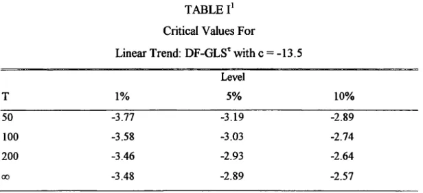
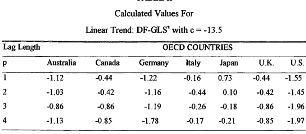
As it can be seen from Tables I and n , for the GNP data under consideration, the sample value o f the DF-GLS^ is greater than the critical values that are obtained by Elliott et al. (1996). Thus, we cannot reject the null hypothesis, which states a univariate time series is integrated o f order one.
TABLE l ' Critical Values For
Linear Trend: DF-GLS^ with c = -13.5
T 1% Level 5% 10% 50 -3.77 -3.19 -2.89 100 -3.58 -3.03 -2.74 200 -3.46 -2.93 -2.64 00 -3.48 -2.89 -2.57
' See Elliott et al. (1996), page 825 for more detailed table. 13
TABLE II Calculated Values For
Linear Trend: DF-GLS^ with c = -13.5
Lag Length OECD COUNTRIES
P Australia Canada Germany Italy Japan U.K. U.S.
1 -1.12 -0.44 -1.22 -0.16 0.73 -0.44 -1.55
2 -1.03 -0.42 -1.16 -0.44 0.10 -0.42 -1.45
3 -0.86 -0.86 -1.19 -0.26 -0.18 -0.86 -1.96
4 -1.13 -0.85 -1.78 -0.17 -0.21 -0.85 -1.97
Table III gives the sample values after 1974 for the same data. Except U.S. for all o f the countries we fail to reject the null by using the critical values indicated in Table I. However, when the level is 5% and p>3 we reject the null hypothesis that states the series is difference stationary. Similarly, at 10 % level when p ^ , we reject the null.
T A B L E m Calculated Values For
Linear Trend: DF-GLS^ with c = -13.5
Lag Length OECD COUNTRIES
P Australia Canada Germany Italy Japan U.K. U.S.
1 -2.04 -1.87 -1.51 -2.13 -1.38 -1.64 -2.66
2 -1.98 -2.04 -1.54 -2.23 -1.36 -2.12 -2.93
3 -2.48 -2.06 -1.67 -2.23 -1.53 -2.64 -3.09
4 -2.01 -1.96 -2.19 -2.44 -1.54 -2.76 -3.38
3.1 Finite Sample Performance
Elliott, Rothenberg, and Stock (1996) conducted a Monte Carlo experiment to see how well the asymptotic theory describes the small-sample properties o f DF- GLS. They investigated tests based on the standard Dickey-Fuller t statistic (denoted DF-T^) and the modified Dickey-Fuller t statistic (denoted DF-GLS^) in the linear trend case. They considered (rit) as a set o f standard normal variables. Although they used the three models for the (vt) process we considered only tw o o f them:
Ut = Ot-l+Vt
I. MA(1): Vt = Tit - 0Tit-i II. AR(1) Vt = <|)Vt-i + Tjt
(0 = .8, .5, 0, -.5, -.8) ((t»= .5, -.5)
(3.1.1) (3.1.2) (3.1.3)
In all o f conditions they considered, since small-sample power typically depends on uo they restrict uo = 0. Although they employed two choices o f lag length, we deal with the one that chooses lag length (p) by the Schwartz (1978) Bayesian information criterion (BIC) constrained so 3<p<8 which is denoted as AR(BIC) estimator.
The results are summarized in Table IV. Tests were at the 5% significance level and the sample size T was 100. For a =1, the table report the observed rejection rates from 5000 Monte Carlo simulations when critical values were based on the limiting distributions. For a < 1, the tables report size-adjusted power, which
is the rejection rate when critical values are estimates from the a =1 Monte Carlo trials.
Table IV shows the size and size-adjusted power o f selected tests o f the 1(1) Null: Monte Carlo Results o f 5% level tests for linear trend for T=100. As it can be observed from the table, DF-GLS^ and DF-t^ have similar size. However, the size- adjusted power o f these tests differs and DF-GLS^ yields better results. For instance, when the power o f the DF-GLS^ is 69%, the power o f DF-x^ stays at 48% with AR(1) coefiBcient is 0.70 in equation 4.3.
The main conclusion that can be obtained from simulations is that the predicted superiority o f the tests using local-to-unity estimates o f the trend parameters is borne out by the Monte Carlo study. The modified Dickey-Fuller tests have higher size-adjusted power than the standard Dickey-Fuller t tests for almost all o f the data generating process.
TABLE IV^
Size and Size-Adjusted Power of Selected Tests of The 1(1) Null; Monte Carlo Results 5% Level Tests, Linear Trend (z* = (l,t)'), T=100
Test Statistic a Asymptotic Power -0.8 MA(1),0= -0.5 0.0 0.5 0.8 AR(1),(|)= 0.5 -0.5 DF-GLSX0.5) 1.00 0.05 0.11 0.08 0.07 0.11 0.58 0.06 0.07 AR(BIC) 0.95 0.10 0.11 0.10 0.10 0.11 0.12 0.10 0.10 0.90 0.27 0.23 0.23 0.24 0.28 0.27 0.22 0.25 0.80 0.81 0.53 0.57 0.61 0.72 0.70 0.48 0.63 0.70 0.99 0.75 0.80 0.84 0.94 0.91 0.69 0.88 DF-x^ 1.00 0.05 0.10 0.07 0.05 0.09 0.58 0.05 0.06 AR(BIC) 0.95 0.09 0.09 0.08 0.08 0.09 0.08 0.08 0.08 0.90 0.19 0.16 0.14 0.15 0.18 0.17 0.14 0.15 0.80 0.61 0.36 0.36 0.39 0.51 0.50 0.30 0.42 0.70 0.94 0.57 0.58 0.64 0.81 0.80 0.48 0.69
See Elliott et al. (1996), page 829 for more detailed Monte Carlo results. 17
Chapter 4
Conclusion
Although lots o f testing procedures developed for testing the hypothesis that a univariate time series is integrated o f order one against the hypothesis that it is integrated o f order zero, no general optimality theory have been developed and the power o f these tests generally questioned in most o f the papers in this field. However, the testing principle developed by Elliott et al.(1996) is one o f the powerful tests in this field.
In our thesis, we applied the testing principle developed by Elliot et al. (1996) by using seasonally unadjusted real GNP o f seven OECD countries; Australia, Canada, Germany, Italy, Japan, U.K., U.S., for two different time period; one for the years between the first quarter o f 1960 and the second quarter o f 1998, and one for the years between the first quarter o f 1974 and the second quarter o f 1998. Although Monte Carlo results - provided by Elliott et al. (1996) - suggest that the DF-GLS test applied to locally de-trended time series has the best overall performance in terms o f small-sample size and power, we caimot reject the hypothesis we have stated before for larger span o f data. However, for the period after 1974 we reject the null for only U.S. when the level is 5%, and 10% when p>3 and p>2, respectively.
SELECT BIBLIOGRAPHY
Ayat, L. and P. Burridge (2000), “ Unit Root Tests in the Presence o f Uncertainty about the Non-Stochastic TxgoA " Journal o f Econometrics, 71-96.
Caner, M., and L. Kilian (2000), “Finite-Sample Critical Values for the Leyboume- McCabe Test o f the Null Hypothesis o f Stationarity,” forthcoming: Journal o f International M oney and Finance.
Cheung, Y.-W., and K. S. Lai (1998), “Parity Reversion in Real Exchange Rates During the Post-Bretton Woods Periods,” Journal o f International M oney and Finance, 17, 597-614.
Cheung, Y. W, and Chinn, M. D. (1996), ‘Turther Investigation o f The Unit Root in GNP,” NBER Technical Working Papers #206.
Diebold, X. Francis and A. Senhadji (1996), “The Uncertain Unit Root in Real GNP: Comment,” The Am erican Economic Review, 86, 264-272.
Elliott, G., Rothenberg, T. J., and Stock, J. H. (1996), “EfiBcient Tests for an Autoregressive Unit Root,” £'cowowc/r/ca, Vol. 64, No. 4, 813-836.
Hamilton, James D. 1994. Time Series Analysis. New Jersey: Princeton University Press.
Rudebusch, G. D. (1993), “The Uncertain Unit Root in Real GNP,” The American Economic Review, 83, 264-272.
APPENDICES
APPENDIX A
THE DATA
AUTRALIA 1960-Ql 26.04 1960-Q2 1960-Q3 1960- Q4 1961- Q l 1961-Q2 1961-Q3 1961- Q4 1962- Q l 1962-Q2 1962-Q3 1962- Q4 1963- Q l 1963-Q2 1963-Q3 1963- Q4 1964- Ql 1964-Q2 1964-Q3 1964- Q4 1965- Q l 1965-Q2 1965-Q3 1965- Q4 1966- Q l 1966-Q2 1966-Q3 1966- Q4 1967- Ql 1967-Q2 1967-Q3 1967- Q4 1968- Q l 1968-Q2 1968-Q3 1968- Q4 1969- Q l 1969-Q2 1969-Q3 1969- Q4 1970- Q l 1970-Q2 1970-Q3 1970- Q4 1971- Ql 1971-Q2 1971-Q3 1971- Q4 1972- Q l 1972-Q2 1972-Q3 1972-Q4 26.09 28.01 27.05 27.07 26.08 27.05 27.05 28.03 28.02 29.04 29.08 30.03 29.02 31.4 31.07 31.05 32.0 33.2 33.9 34.1 34.2 34.8 34.7 34.5 34.4 36.5 36.7 37.7 37.0 38.5 38.7 38.0 38.9 41.2 42.4 42.0 42.2 43.4 44.4 44.7 45.5 46.0 46.6 46.9 47.0 48.3 48.6 47.7 48.9 48.6 49.5 1973-Ql 1973-Q2 1973-Q3 1973- Q4 1974- Q l 1974-Q2 1974-Q3 1974- Q4 1975- Q l 1975-Q2 1975-Q3 1975- Q4 1976- Q l 1976-Q2 1976-Q3 1976- Q4 1977- Q l 1977-Q2 1977-Q3 1977- Q4 1978- Q l 1978-Q2 1978-Q3 1978- Q4 1979- Q l 1979-Q2 1979-Q3 1979- Q4 1980- Q l 1980-Q2 1980-Q3 1980- Q4 1981- Q l 1981-Q2 1981-Q3 1981- Q4 1982- Q l 1982-Q2 1982-Q3 1982- Q4 1983- Q l 1983-Q2 1983-Q3 1983- Q4 1984- Q l 1984-Q2 1984-Q3 1984- Q4 1985- Q l 1985-Q2 1985-Q3 1985-Q4 50.5 50.7 51.4 53.1 53.6 52.1 52.6 53.1 53.1 53.5 53.9 54.1 54.8 55.5 56.2 56.2 56.5 56.9 57.0 56.5 57.0 58.1 58.8 59.4 61.9 60.4 60.7 62.3 61.7 61.7 62.5 63.4 63.2 64.6 65.4 65.9 65.8 66.0 65.3 64.1 63.6 63.7 65.6 67.8 68.5 69.2 69.9 70.1 71.6 72.8 73.9 74.1 1986-Ql 1986-Q2 1986-Q3 1986- Q4 1987- Q l 1987-Q2 1987-Q3 1987- Q4 1988- Ql 1988-Q2 1988-Q3 1988- Q4 1989- Ql 1989-Q2 1989-Q3 1989- Q4 1990- Q l 1990-Q2 1990-Q3 1990- Q4 1991- Ql 1991-Q2 1991-Q3 1991- Q4 1992- Q l 1992-Q2 1992-Q3 1992- Q4 1993- Q l 1993-Q2 1993-Q3 1993- Q4 1994- Q l 1994-Q2 1994-Q3 1994- Q4 1995- Ql 1995-Q2 1995-Q3 1995- Q4 1996- Ql 1996-Q2 1996-Q3 1996- Q4 1997- Ql 1997-Q2 1997-Q3 1997- Q4 1998- Q l 1998-Q2 74.4 74.1 74.6 75.9 76.6 77.7 78.9 80.5 80.8 81.0 81.8 83.3 83.9 85.7 86.0 86.2 87.1 87.4 86.6 87.0 86.4 85.8 85.9 86.2 87.2 87.4 88.4 89.4 90.7 91.1 91.1 92.7 95.0 95.6 97.1 97.7 97.9 99.3 101.0 101.8 103.3 103.0 104.1 105.1 105.5 107.5 108.3 109.7 111.2 112.5 21CANADA 1960-Ql 1960-Q2 1960-Q3 1960- Q4 1961- Q l 1961-Q2 1961-Q3 1961- Q4 1962- Ql 1962-Q2 1962-Q3 1962- Q4 1963- Ql 1963-Q2 1963-Q3 1963- Q4 1964- Q l 1964-Q2 1964-Q3 1964- Q4 1965- Q l 1965-Q2 1965-Q3 1965- Q4 1966- Q l 1966-Q2 1966-Q3 1966- Q4 1967- Q l 1967-Q2 1967-Q3 1967- Q4 1968- Q l 1968-Q2 1968-Q3 1968- Q4 1969- Q l 1969-Q2 1969-Q3 1969- Q4 1970- Q l 1970-Q2 1970-Q3 1970- Q4 1971- Q l 1971-Q2 1971-Q3 1971- Q4 1972- Q l 1972-Q2 1972-Q3 1972-Q4 27.01 26.06 27.0 27.01 26.09 27.06 28.01 28.06 29.04 29.04 29.09 30.04 30.06 31.0 31.04 32.4 33.0 33.1 33.6 33.8 34.9 35.2 35.7 36.6 37.5 38.0 38.1 38.5 38.4 39.2 39.4 39.5 39.9 40.9 41.6 42.5 42.8 43.0 43.6 44.4 44.4 44.1 44.9 44.9 45.3 46.7 48.1 48.6 48.4 49.7 49.9 51.3 1973-Ql 1973-Q2 1973-Q3 1973- Q4 1974- Q l 1974-Q2 1974-Q3 1974- Q4 1975- Q l 1975-Q2 1975-Q3 1975- Q4 1976- Q l 1976-Q2 1976-Q3 1976- Q4 1977- Q l 1977-Q2 1977-Q3 1977- Q4 1978- Q l 1978-Q2 1978-Q3 1978- Q4 1979- Q l 1979-Q2 1979-Q3 1979- Q4 1980- Q l 1980-Q2 1980-Q3 1980- Q4 1981- Q l 1981-Q2 1981-Q3 1981- Q4 1982- Q l 1982-Q2 1982-Q3 1982- Q4 1983- Q l 1983-Q2 1983-Q3 1983- Q4 1984- Q l 1984-Q2 1984-Q3 1984- Q4 1985- Q l 1985-Q2 1985-Q3 1985-Q4 52.9 53.3 53.5 55.0 55.5 55.9 56.2 56.6 56.5 57.1 57.9 58.5 59.8 61.2 61.6 61.6 62.6 62.8 63.2 64.4 65.0 66.0 66.4 67.2 68.0 68.4 69.1 69.4 69.6 69.5 69.2 70.6 72.1 73.0 72.3 71.8 71.0 70.1 69.7 69.1 70.3 71.9 73.0 73.6 74.8 76.5 77.4 78.3 79.2 79.5 80.5 82.3 1986-Ql 1986-Q2 1986-Q3 1986- Q4 1987- Q l 1987-Q2 1987-Q3 1987- Q4 1988- Q l 1988-Q2 1988-Q3 1988- Q4 1989- Ql 1989-Q2 1989-Q3 1989- Q4 1990- Q l 1990-Q2 1990-Q3 1990- Q4 1991- Q l 1991-Q2 1991-Q3 1991- Q4 1992- Q l 1992-Q2 1992-Q3 1992- Q4 1993- Q l 1993-Q2 1993-Q3 1993- Q4 1994- Ql 1994-Q2 1994-Q3 1994- Q4 1995- Ql 1995-Q2 1995-Q3 1995- Q4 1996- Q l 1996-Q2 1996-Q3 1996- Q4 1997- Ql 1997-Q2 1997-Q3 1997- Q4 1998- Q l 1998-Q2 82.8 83.0 83.4 83.1 85.1 85.6 87.3 88.4 89.6 90.8 91.1 91.8 92.7 92.9 93.2 93.3 93.7 93.3 92.8 91.6 90.4 91.2 91.4 91.6 91.6 91.9 91.9 92.0 92.9 93.7 94.1 94.9 95.9 97.0 98.4 99.6 100.8 99.7 99.9 100.3 100.4 100.6 102.5 103.1 104.4 105.7 106.8 107.6 108.4 108.8 22
G ERM ANY 1960-Ql 1960-Q2 1960-Q3 1960- Q4 1961- Q l 1961-Q2 1961-Q3 1961- Q4 1962- Ql 1962-Q2 1962-Q3 1962- Q4 1963- Q l 1963-Q2 1963-Q3 1963- Q4 1964- Q l 1964-Q2 1964-Q3 1964- Q4 1965- Q l 1965-Q2 1965-Q3 1965- Q4 1966- Q l 1966-Q2 1966-Q3 1966- Q4 1967- Q l 1967-Q2 1967-Q3 1967- Q4 1968- Q l 1968-Q2 1968-Q3 1968- Q4 1969- Q l 1969-Q2 1969-Q3 1969- Q4 1970- Q l 1970-Q2 1970-Q3 1970- Q4 1971- Q l 1971-Q2 1971-Q3 1971- Q4 1972- Q l 1972-Q2 1972-Q3 1972-Q4 32.0 32.5 33.7 34.0 34.4 34.2 34.9 35.0 35.5 35.9 36.8 36.7 35.4 37.0 38.3 38.5 39.0 39.5 39.9 40.4 41.1 41.7 42.0 42.3 43.0 43.2 43.2 42.5 42.3 42.2 43.2 43.8 42.9 45.0 45.8 47.3 46.3 48.4 49.2 50.7 49.2 51.2 51.3 52.4 51.6 52.6 52.8 53.2 53.8 54.3 55.1 56.2 1973-Ql 57.2 1986-Ql 71.2 1973-Q2 57.3 1986-Q2 72.2 1973-Q3 57.7 1986-Q3 72.9 1973-Q4 57.7 1986-Q4 73.5 1974-Ql 58.1 1987-Ql 71.5 1974-Q2 57.9 1987-Q2 73.4 1974-Q3 57.7 1987-Q3 73.9 1974-Q4 56.9 1987-Q4 74.8 1975-Ql 56.6 1988-Ql 74.8 1975-Q2 56.4 1988-Q2 75.4 1975-Q3 56.9 1988-Q3 76.6 1975-Q4 57.8 1988-Q4 77.5 1976-Ql 58.9 1989-Ql 78.3 1976-Q2 59.7 1989-Q2 78.3 1976-Q3 59.3 1989-Q3 78.9 1976-Q4 61.0 1989-Q4 79.9 1977-Ql 61.1 1990-Ql 81.9 1977-Q2 61.3 1990-Q2 82.7 1977-Q3 61.0 1990-Q3 84.1 1977-Q4 62.8 1990-Q4 85.5 1978-Ql 62.8 1991-Ql 94.4 1978-Q2 62.8 1991-Q2 94.8 1978-Q3 63.4 1991-Q3 94.3 1978-Q4 64.7 1991-Q4 95.1 1979-Ql 64.5 1992-Ql 96.9 1979-Q2 66.6 1992-Q2 96.3 1979-Q3 66.5 1992-Q3 96.2 1979-Q4 66.9 1992-Q4 96.0 1980-Ql 67.5 1993-Ql 94.7 1980-Q2 66.9 1993-Q2 94.7 1980-Q3 66.4 1993-Q3 95.7 1980-Q4 66.2 1993-Q4 95.8 1981-Ql 66.9 1994-Ql 96.9 1981-Q2 66.9 1994-Q2 97.4 1981-Q3 66.9 1994-Q3 98.0 1981-Q4 66.6 1994-Q4 99.1 1982-Ql 66.7 1995-Ql 98.7 1982-Q2 66.5 1995-Q2 99.4 1982-Q3 65.6 1995-Q3 99.2 1982-Q4 65.7 1995-Q4 99.1 1983-Ql 66.6 1996-Ql 99.1 1983-Q2 67.2 1996-Q2 100.4 1983-Q3 67.1 1996-Q3 100.8 1983-Q4 68.3 1996-Q4 101.2 1984-Ql 69.1 1997-Ql 101.6 1984-Q2 68.0 1997-Q2 102.6 1984-Q3 69.7 1997-Q3 103.2 1984-Q4 70.0 1997-Q4 103.5 1985-Ql 69.7 1998-Ql 105.0 1985-Q2 70.5 1998-Q2 105.0 1985-Q3 71.4 1985-Q4 71.6 23
ITA LY 1960-Ql 1960-Q2 1960-Q3 1960- Q4 1961- Q l 1961-Q2 1961-Q3 1961- Q4 1962- Q l 1962-Q2 1962-Q3 1962- Q4 1963- Q l 1963-Q2 1963-Q3 1963- Q4 1964- Q l 1964-Q2 1964-Q3 1964- Q4 1965- Q l 1965-Q2 1965-Q3 1965- Q4 1966- Q l 1966-Q2 1966-Q3 1966- Q4 1967- Q l 1967-Q2 1967-Q3 1967- Q4 1968- Q l 1968-Q2 1968-Q3 1968- Q4 1969- Q l 1969-Q2 1969-Q3 1969- Q4 1970- Q l 1970-Q2 1970-Q3 1970- Q4 1971- Q l 1971-Q2 1971-Q3 1971- Q4 1972- Q l 1972-Q2 1972-Q3 1972-Q4 28.01 28.06 28.09 29.0 30.0 30.07 31.4 31.9 32.4 32.8 33.0 33.5 33.5 34.5 35.2 35.7 36.0 35.6 35.5 35.4 35.9 36.6 37.0 37.6 40.7 41.3 42.4 42.6 43.5 44.4 45.1 46.0 46.1 47.1 48.2 49.3 50.1 51.0 51.1 50.1 52.4 53.1 53.9 53.7 53.9 53.9 54.5 54.9 55.7 55.5 55.9 56.4 1973-Ql 1973-Q2 1973-Q3 1973- Q4 1974- Q l 1974-Q2 1974-Q3 1974- Q4 1975- Q l 1975-Q2 1975-Q3 1975- Q4 1976- Q l 1976-Q2 1976-Q3 1976- Q4 1977- Q l 1977-Q2 1977-Q3 1977- Q4 1978- Q l 1978-Q2 1978-Q3 1978- Q4 1979- Q l 1979-Q2 1979-Q3 1979- Q4 1980- Q l 1980-Q2 1980-Q3 1980- Q4 1981- Q l 1981-Q2 1981-Q3 1981- Q4 1982- Q l 1982-Q2 1982-Q3 1982- Q4 1983- Q l 1983-Q2 1983-Q3 1983- Q4 1984- Q l 1984-Q2 1984-Q3 1984- Q4 1985- Q l 1985-Q2 1985-Q3 1985-Q4 57.2 58.7 60.7 61.6 62.8 62.8 62.6 61.1 60.4 60.3 61.2 62.1 62.9 64.3 65.8 66.8 67.2 66.9 66.5 66.7 68.0 68.7 69.6 71.0 71.8 72.2 73.4 75.6 76.2 76.2 75.4 75.6 75.5 76.4 76.4 76.5 76.6 76.8 76.4 76.3 76.7 77.0 77.6 78.6 79.4 79.4 79.5 79.7 80.4 81.4 82.1 82.8 1986-Ql 1986-Q2 1986-Q3 1986- Q4 1987- Ql 1987-Q2 1987-Q3 1987- Q4 1988- Ql 1988-Q2 1988-Q3 1988- Q4 1989- Ql 1989-Q2 1989-Q3 1989- Q4 1990- Ql 1990-Q2 1990-Q3 1990- Q4 1991- Q l 1991-Q2 1991-Q3 1991- Q4 1992- Q l 1992-Q2 1992-Q3 1992- Q4 1993- Q l 1993-Q2 1993-Q3 1993- Q4 1994- Q l 1994-Q2 1994-Q3 1994- Q4 1995- Q l 1995-Q2 1995-Q3 1995- Q4 1996- Ql 1996-Q2 1996-Q3 1996- Q4 1997- Q l 1997-Q2 1997-Q3 1997- Q4 1998- Q l 1998-Q2 82.9 83.8 84.6 84.9 85.1 86.5 86.9 88.1 89.1 89.6 90.2 91.1 91.6 92.1 92.7 93.9 94.4 94.5 94.9 94.5 95.0 95.3 96.0 96.3 96.5 96.6 96.1 95.5 94.9 95.0 94.8 95.6 96.0 97.0 97.6 98.0 99.7 99.6 100.2 100.6 101.4 100.3 100.6 100.3 100.5 102.3 102.8 103.1 102.9 103.5 24
JAPAN 1960-Ql 1960-Q2 1960-Q3 1960- Q4 1961- Q l 1961-Q2 1961-Q3 1961- Q4 1962- Q l 1962-Q2 1962-Q3 1962- Q4 1963- Q l 1963-Q2 1963-Q3 1963- Q4 1964- Q l 1964-Q2 1964-Q3 1964- Q4 1965- Q l 1965-Q2 1965-Q3 1965- Q4 1966- Q l 1966-Q2 1966-Q3 1966- Q4 1967- Q l 1967-Q2 1967-Q3 1967- Q4 1968- Q l 1968-Q2 1968-Q3 1968- Q4 1969- Q l 1969-Q2 1969-Q3 1969- Q4 1970- Q l 1970-Q2 1970-Q3 1970- Q4 1971- Q l 1971-Q2 1971-Q3 1971- Q4 1972- Q l 1972-Q2 1972-Q3 1972-Q4 16.05 16.05 17.01 17.08 18.03 18.07 19.0 19.09 20.02 20.05 20.08 21.01 21.04 22.0 22.07 23.04 24.02 24.09 25.02 25.05 25.07 26.01 26.07 27.0 27.08 29.0 29.07 30.2 31.0 31.08 32.9 33.6 34.3 35.6 36.4 38.7 38.9 40.0 40.9 42.7 43.9 44.3 45.6 45.5 45.7 46.4 47.2 47.7 49.0 50.0 51.0 52.2 1973-Ql 1973-Q2 1973-Q3 1973- Q4 1974- Ql 1974-Q2 1974-Q3 1974- Q4 1975- Ql 1975-Q2 1975-Q3 1975- Q4 1976- Ql 1976-Q2 1976-Q3 1976- Q4 1977- Q l 1977-Q2 1977-Q3 1977- Q4 1978- Q l 1978-Q2 1978-Q3 1978- Q4 1979- Ql 1979-Q2 1979-Q3 1979- Q4 1980- Q l 1980-Q2 1980-Q3 1980- Q4 1981- Q l 1981-Q2 1981-Q3 1981- Q4 1982- Q l 1982-Q2 1982-Q3 1982- Q4 1983- Ql 1983-Q2 1983-Q3 1983- Q4 1984- Q l 1984-Q2 1984-Q3 1984- Q4 1985- Ql 1985-Q2 1985-Q3 1985-Q4 53.9 54.5 54.5 54.9 53.5 54.0 54.7 54.3 54.2 55.6 56.1 56.8 57.3 57.7 58.5 58.6 60.0 60.5 60.8 61.7 62.7 63.2 64.1 64.9 58.8 59.8 60.4 60.9 61.8 61.7 62.2 63.0 64.0 64.0 64.7 64.9 65.6 66.4 66.7 67.3 67.6 67.7 68.8 69.0 70.1 71.1 71.5 72.1 73.2 74.5 75.0 76.1 1986-Ql 1986-Q2 1986-Q3 1986- Q4 1987- Ql 1987-Q2 1987-Q3 1987- Q4 1988- Ql 1988-Q2 1988-Q3 1988- Q4 1989- Ql 1989-Q2 1989-Q3 1989- Q4 1990- Ql 1990-Q2 1990-Q3 1990- Q4 1991- Q l 1991-Q2 1991-Q3 1991- Q4 1992- Ql 1992-Q2 1992-Q3 1992- Q4 1993- Ql 1993-Q2 1993-Q3 1993- Q4 1994- Ql 1994-Q2 1994-Q3 1994- Q4 1995- Q l 1995-Q2 1995-Q3 1995- Q4 1996- Ql 1996-Q2 1996-Q3 1996- Q4 1997- Ql 1997-Q2 1997-Q3 1997- Q4 1998- Ql 1998-Q2 75.3 76.5 77.0 78.0 78.3 78.7 80.1 81.9 83.2 83.8 85.5 86.6 87.7 87.6 89.3 90.4 90.8 92.7 93.8 95.0 96.0 96.6 96.9 97.7 98.3 98.0 97.5 97.5 97.6 97.9 98.1 98.0 98.0 98.5 99.1 98.8 98.3 99.8 100.5 101.2 103.9 104.0 103.6 104.7 106.8 103.8 104.6 104.2 104.4 103.7 25
υ.κ.
1960-Ql 1960-Q2 1960-Q3 1960- Q4 1961- Q l 1961-Q2 1961-Q3 1961- Q4 1962- Q l 1962-Q2 1962-Q3 1962- Q4 1963- Ql 1963-Q2 1963-Q3 1963- Q4 1964- Ql 1964-Q2 1964-Q3 1964- Q4 1965- Q l 1965-Q2 1965-Q3 1965- Q4 1966- Q l 1966-Q2 1966-Q3 1966- Q4 1967- Ql 1967-Q2 1967-Q3 1967- Q4 1968- Q l 1968-Q2 1968-Q3 1968- Q4 1969- Q l 1969-Q2 1969-Q3 1969- Q4 1970- Q l 1970-Q2 1970-Q3 1970- Q4 1971- Q l 1971-Q2 1971-Q3 1971- Q4 1972- Q l 1972-Q2 1972-Q3 1972-Q4 44.9 44.6 45.2 45.3 46.0 46.3 46.2 46.0 46.2 46.8 47.2 46.9 46.8 48.7 49.0 49.9 50.5 51.1 51.1 52.3 52.3 52.1 52.5 53.2 53.3 53.5 53.6 53.7 54.3 54.8 54.8 55.1 57.0 56.2 57.2 57.6 57.6 58.0 58.3 58.7 58.4 59.5 59.9 60.2 59.6 60.5 61.3 61.4 61.1 62.8 62.9 64.3 1973-Ql 1973-Q2 1973-Q3 1973- Q4 1974- Q l 1974-Q2 1974-Q3 1974- Q4 1975- Q l 1975-Q2 1975-Q3 1975- Q4 1976- Q l 1976-Q2 1976-Q3 1976- Q4 1977- Q l 1977-Q2 1977-Q3 1977- Q4 1978- Q l 1978-Q2 1978-Q3 1978- Q4 1979- Q l 1979-Q2 1979-Q3 1979- Q4 1980- Q l 1980-Q2 1980-Q3 1980- Q4 1981- Q l 1981-Q2 1981-Q3 1981- Q4 1982- Q l 1982-Q2 1982-Q3 1982- Q4 1983- Q l 1983-Q2 1983-Q3 1983- Q4 1984- Q l 1984-Q2 1984-Q3 1984- Q4 1985- Ql 1985-Q2 1985-Q3 1985-Q4 67.5 67.6 67.7 66.9 65.2 66.6 67.2 66.1 66.4 65.6 65.4 65.9 67.3 66.9 67.5 68.9 68.8 68.6 69.2 70.2 70.7 71.4 72.0 72.4 72.0 75.1 73.4 74.0 73.6 72.1 71.6 70.8 70.7 70.6 71.5 71.6 71.7 72.3 72.4 72.8 74.3 74.5 75.2 76.0 76.8 76.4 76.4 77.3 78.5 79.7 79.9 80.4 1986-Ql 1986-Q2 1986-Q3 1986- Q4 1987- Q l 1987-Q2 1987-Q3 1987- Q4 1988- Ql 1988-Q2 1988-Q3 1988- Q4 1989- Ql 1989-Q2 1989-Q3 1989- Q4 1990- Q l 1990-Q2 1990-Q3 1990- Q4 1991- Q l 1991-Q2 1991-Q3 1991- Q4 1992- Q l 1992-Q2 1992-Q3 1992- Q4 1993- Q l 1993-Q2 1993-Q3 1993- Q4 1994- Ql 1994-Q2 1994-Q3 1994- Q4 1995- Q l 1995-Q2 1995-Q3 1995- Q4 1996- Q l 1996-Q2 1996-Q3 1996- Q4 1997- Ql 1997-Q2 1997-Q3 1997- Q4 1998- Ql 1998-Q2 81.5 82.5 83.5 84.7 85.2 86.3 87.8 88.8 90.1 90.6 92.0 92.8 93.1 93.4 93.5 93.6 94.0 94.5 93.6 92.8 92.4 91.8 91.6 91.8 91.1 91.2 91.6 91.7 92.6 92.8 93.7 94.4 95.5 96.6 97.6 98.3 98.7 99.1 99.7 100.1 100.4 101.8 102.5 103.5 104.3 105.3 106.2 106.8 107.6 108.1 26u.s.
1960-Ql 1960-Q2 1960-Q3 1960- Q4 1961- Ql 1961-Q2 1961-Q3 1961- Q4 1962- Q l 1962-Q2 1962-Q3 1962- Q4 1963- Q l 1963-Q2 1963-Q3 1963- Q4 1964- Q l 1964-Q2 1964-Q3 1964- Q4 1965- Q l 1965-Q2 1965-Q3 1965- Q4 1966- Q l 1966-Q2 1966-Q3 1966- Q4 1967- Q l 1967-Q2 1967-Q3 1967- Q4 1968- Q l 1968-Q2 1968-Q3 1968- Q4 1969- Q l 1969-Q2 1969-Q3 1969- Q4 1970- Q l 1970-Q2 1970-Q3 1970- Q4 1971- Q l 1971-Q2 1971-Q3 1971- Q4 1972- Q l 1972-Q2 1972-Q3 1972-Q4 33.7 33.5 33.5 33.1 33.3 33.9 34.5 35.2 35.8 36.2 36.6 36.6 37.1 37.5 38.2 38.5 39.4 39.9 40.4 40.5 41.5 42.1 42.9 43.9 45.0 45.2 45.5 45.9 46.2 46.3 46.6 47.0 47.9 48.7 49.0 49.3 50.0 50.1 50.4 50.2 50.1 50.2 50.6 50.1 51.5 51.8 52.1 52.3 53.3 54.5 55.1 56.1 1973-Ql 1973-Q2 1973-Q3 1973- Q4 1974- Q l 1974-Q2 1974-Q3 1974- Q4 1975- Q l 1975-Q2 1975-Q3 1975- Q4 1976- Q l 1976-Q2 1976-Q3 1976- Q4 1977- Q l 1977-Q2 1977-Q3 1977- Q4 1978- Q l 1978-Q2 1978-Q3 1978- Q4 1979- Q l 1979-Q2 1979-Q3 1979- Q4 1980- Q l 1980-Q2 1980-Q3 1980- Q4 1981- Q l 1981-Q2 1981-Q3 1981- Q4 1982- Q l 1982-Q2 1982-Q3 1982- Q4 1983- Q l 1983-Q2 1983-Q3 1983- Q4 1984- Q l 1984-Q2 1984-Q3 1984- Q4 1985- Q l 1985-Q2 1985-Q3 1985-Q4 57.6 58.0 57.8 58.4 57.8 58.0 57.4 57.0 56.2 56.7 57.8 58.5 59.8 60.2 60.5 61.0 61.8 63.0 64.0 64.0 64.3 66.7 67.3 68.1 68.1 68.3 68.7 68.9 69.2 67.5 67.5 68.8 70.1 69.5 70.3 69.4 68.3 68.5 68.2 68.3 69.0 70.4 71.7 73.0 74.7 75.9 76.5 77.0 77.8 78.1 79.3 79.8 1986-Ql 1986-Q2 1986-Q3 1986- Q4 1987- Q l 1987-Q2 1987-Q3 1987- Q4 1988- Q l 1988-Q2 1988-Q3 1988- Q4 1989- Q l 1989-Q2 1989-Q3 1989- Q4 1990- Ql 1990-Q2 1990-Q3 1990- Q4 1991- Q l 1991-Q2 1991-Q3 1991- Q4 1992- Q l 1992-Q2 1992-Q3 1992- Q4 1993- Q l 1993-Q2 1993-Q3 1993- Q4 1994- Q l 1994-Q2 1994-Q3 1994- Q4 1995- Q l 1995-Q2 1995-Q3 1995- Q4 1996- Q l 1996-Q2 1996-Q3 1996- Q4 1997- Ql 1997-Q2 1997-Q3 1997- Q4 1998- Ql 1998-Q2 80.8 80.9 81.3 81.7 82.3 83.1 83.8 85.0 85.6 86.4 86.9 88.0 88.9 89.6 90.0 90.1 91.0 91.3 90.8 89.9 89.4 89.8 90.1 90.3 91.3 91.9 92.6 92.3 93.6 94.1 94.6 95.8 96.5 97.6 98.0 98.9 99.3 99.4 100.3 100.9 101.8 103.3 103.8 104.9 106.0 107.0 108.1 108.9 110.4 110.9 27APPENDIX B
FIGURES
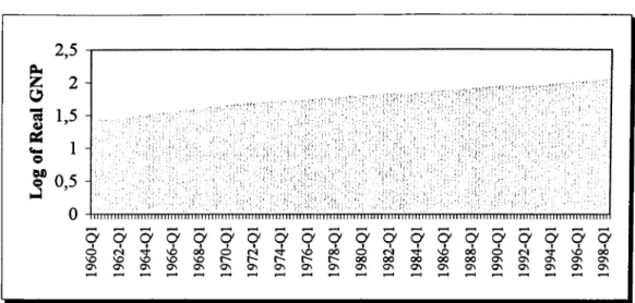
Figure B. 1. Real GNP o f Australia
Z o
■a
o OD
Figure B.2. Real GNP o f Canada
Pui o "3 o M) o 28
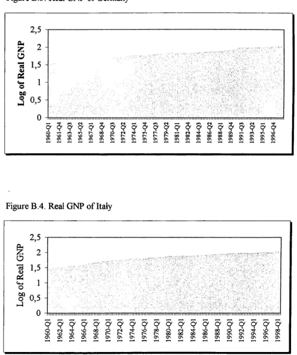
Figure B .3. Real GNP o f Germany Pm
§
*c3 £ O OX) oFigure B.4, Real GNP o f Italy
O ' S o 00 o 29
03 о 1 9 6 0 - Q l 1 9 6 1 - Q 4 1 9 6 3 -Q 3 1 9 6 5 -Q 2 1 9 6 7 - Q l 1 9 6 8 - Q 4 1 9 7 0 -Q 3 1 9 7 2 -Q 2 1 9 7 4 - Q l 1 9 7 5 - Q 4 1 9 7 7 -Q 3 1 9 7 9 -Q 2 1 9 8 1 - Q l 1 9 8 2 - Q 4 1 9 8 4 -Q 3 1 9 8 6 -Q 2 1 9 8 8 - Q l 1 9 8 9 - Q 4 1 9 9 1 -Q 3 1 9 9 3 -Q 2 1 9 9 5 - Q l 1 9 9 6 - Q 4 L o g o f R e a l G N P о J> о Ί λ ^ b J \ 4- -- 1 -1_ __ __ 1_ __ -J . . J л h cj f 3 o \ σ ^ С L o f o f R e a l G N P o ^ N NJ NJ D ^ » u » to u i .■ 1 9 6 0 -Q 1 : Ξ . - ; 1 9 6 1 -Q 4 1 E
i
1 9 6 3 -Q 3 1 j . ^ ' 1 9 6 5 -Q 2 1 j о '-Ъ 1 9 6 7 -Q 1 1 . : ■■ ■ ■■ r- - ■ dИ
1 9 6 8 -Q 4 1 Γ 1 9 7 0 -Q 3 1 Ι ' -. ' 1 9 7 2 -Q 2 1 1 9 7 4 -Q 1 1 1 1 9 7 5 -Q 4 1 1 1 9 7 7 -Q 3 1 z ■ ■ · . ■ . . .... . . . .... ... 1 9 7 9 -Q 2 Î 1 ' _ . / ' 1 9 8 1 -Q 1 І 1 9 8 2 -Q 4 I 1 9 8 4 -Q 3 1 1 ■' ;■ ·'· 1 9 8 6 -Q 2 i y : 1 9 8 8 -Q l I ·'. ,■ . '·■ ' ■. / 1 ' ; 1 9 8 9 -Q 4 i 1 9 9 1 -Q 3 I 1 ^ ул ': у > -ч '· 1 9 9 3 -Q 2 1 - ' -y . . 1 9 9 5 -Q l 1 - - ' / " 'r. 1 - ■ 1 9 9 6 -Q 4 I f 3 о о «o> L o g o f R e a l G N P о N o ·— » to LT » 1 О ЛП ni İ l i l IV O U -v ^l ; 19 62 -Q l \ 19 64 -Q l Ξ 19 66 -Q l Ξ 19 68 -Q l Ξ 19 70 -Q l \ ’> ¿1 19 72 -Q l 1 19 74 -Q l \ 19 76 -Q l i 19 78 -Q l i 19 80 -Q l 1 19 82 -Q l i 19 84 -Q l ! 19 86 -Q l i 19 88 -Q l 1 19 90 -Q l i 19 92 -Q l l 19 94 -Q l \ 19 96 -Q l i 19 98 -0 1 = 'S ' о Os <1 Й. 0 o *-b G СЛ
APPENDIX C
Gauss Program
load dat[154,l]=italy.txt;
P =i;
pmax=4; dfgs=zeros^max, 1); do while p<=^max;
ou^ut file=ausq.out reset; y=ln(dat); t=rows(dat); rbar=l+(-13.5/t); yb=zeros(t,l); yb[2:t]=y[2t]-(rbar*y[l i-1]); yb=y[l]|yb[2;t]; z=ones(t, l)~seqa(l, 1 ,t); zb=zeros(t,2); zb[2.t.,]=z[2t,.]-(rbar.*z[l:t-l,.]); zb=z[l,.]|zb[2A,.]; beta=inv(zb'zb)*zb'*yb; y=y-z*beta; dy=y[2t]-y[l:t-l]; x=yb>+l :t-l]~dy0).t-2]; ki=2; do \diile k i< ^ ; x=x~dy|p+l-ki:t-l-ki]; ki=ki+l; endo; 32
b=inv(x'x)*x'*dy[p+l dc=zeros^,l); ep={l}; ep=ep~dc'; A o=^*b; res=dy[p+l l-l]-(x*b); s2=res'res/(t-p-l); xx=inv(x'x); den=sqrt(diag(xx)*s2); dfgs[p]=Ao/den[l]; p=p+l; «ido; dfgs; 33