Solution of feasibility problems via non-smooth optimization

SOLUTION OF FEASiBİLir/ PROBLEMS

VIA NON-SMOOTH Ό ΡΤΙΜ Ι2.ΑΤΙ0 Μ

A ■ ε c 5 ς іГЧ» n я яяи.. f . - « r e a r » · · » « я ;. *--Г*ДГ^ ■T?·-'! 3 ■?" ·«“ ·?· * ♦ ? · ' ^ » » * . л -«·ι- fr ί w . ^ -è -t »İ» ! i .{! ІЯ J ι··τ .k à ■ .·) K Ч '» ·’“ ■< ·►* 4 j r*»*· ¿ i’·· -f·? !· 'P j j “ “ '' Ч, îî T \» Ÿ ii Ч « » w * іа-і? I J ·^ á 5' .1»· ù! fcto.lâa«*' ii ' W ' «f « Í і і н , s a » a . « І V i i.us a ^3 ь 'I W i- « 4 V *«V · W a т . я · » » » u 3 ІГ- _{3htf^ à \} :3cJî ^'Т:і Λ i 'd -ijf к Ш і ¿."i . >:' j: -rP5 r, ¡1^ J ^ 3 >■·»« ίί*«|Η» ’} ?· i f“;“: -■’*"<-■ ■·■ и ? ··■* J *;! aJ J .î» Э.2V« Ча»* w w w ms·' w .

’**“ /·« ^

■ ВЫ ОіШ ЕЕ^Ш й *T -T** l**’-f“··;,/ i s .«41 P

SOLUTION OF FEASIBILITY PROBLEMS

VIA NON-SMOOTH OPTIMIZATION

A THESIS

SUBMITTED TO THE DEPARTMENT OF INDUSTRIAL ENGINEERING AND THE INSTITUTE OF ENGINEERING AND SCIENCES

OF BILKENT UNIVERSITY

IN PARTIAL FULFILLMENT OF THE REQUIREMENTS FOR THE DEGREE OF

MASTER OF SCIENCE

By

Iradj Ouveysi December, 1990 ___

---■

' '-ir.

( j } \

2 М

@ Copyright December, 1990 by

Iradj Ouveysi

I certify that I have read this thesis and that in my opinion it is fully ade­ quate, in scope and in quality, as a thesis for the degree of Master of Science.

Associate Prof. Dr. Osman (Principal Advisor)

I certify that I have read this thesis and that in my opinion it is fully ade­ quate, in scope and in quality, as'a thesis for the degree of Master of Science.

/

_______ V / X V/ _______

Associat^'-Prof. Dr. ^ustafa Akgiil

I certify that I have read this thesis and that in my opinion it is fully ade­ quate, in scope and in quality, as a thesis for the degree of Master of Science.

Z

'..j

Prof. D r/ Halim Doğ:rusoz

I certify that I have read this thesis and that in my opinion it is fully ade­ quate, in scope and in quality, as a thesis for the degree of Master of Science.

v M A 4 X

-Prof. Dr. A1Akif Eyler

I certify that I have read this thesis and that in my opinion it is fully ade­ quate, in scope and in quality, as a thesis for the degree of Master of Science.

Associate Prof. Dr. Peter Kas

Approved for the Institute of Engineering and Sciences:

Prof. Mehrqirt BeBar ay

Director of Institute of Engineering and Sciences

ABSTRACT

S O L U T IO N O F F E A S IB IL IT Y P R O B L E M S V I A N O N -S M O O T H O P T IM IZ A T IO N

Iradj Ouveysi

M .S . in Industrial Engineering

Supervisor: Associate Prof. Dr. Osman Oğuz

December, 1990

In this study we present a penalty function approach for linear feasibility problems. Our attempt is to find an eiL· coive algorithm based on an exterior method. Any given feasibility (for a set o f linear inequalities) problem, is first transformed into an unconstrained minimization o f a penalty function, and then the problem is reduced to minimizing a convex, non-smooth, quadratic function. Due to non-differentiability o f the penalty function, the gradient type methods can not be applied directly, so a modified nonlinear programming technique will be used in order to overcome the difficulties o f the break points. In this research we present a new algorithm for minimizing this non-smooth penalty function.

By dropping the nonnegativity constraints and using conjugate gradient method we compute a maxi­ mum set o f conjugate directions and then we perform line searches on these directions in order to minimize our penalty function. Whenever the optimality criteria is not satisfied and the improvements in all direc­ tions are not enough, we calculate the new set o f conjugate directions by conjugate Gram Schmit process, but one o f the directions is the element o f sub differential at the present point.

K ey w ’o rd s : Non-Smooth Optimization, Nonlinear Programming, Linear Programming, Feasibility Problem, Penalty Function.

ÖZET

’’ F E A S I B I L IT Y ” P R O B L E M L E R İN İN Ç Ö Z Ü M Ü N D E Y E N İ B İR C E Z A F O N K S İ Y O N U M E T O D U

Iradj Ouveysi

Endüstri Mühendisliği Bölüm ü Yüksek Lisans Tez Yöneticisi: Doç. O sm an Oğuz

Aralık, 1990

Bu çalışmada, doğrusal uyumluluk (feeısibility) problemleri için, ceza fonksiyonu yöntemine dayalı yeni bir yaklaşım sunuyoruz. Amacımız, dışsal metod ilkesiyle çalışan etkili bir algoritma bulmaktır. Geliştirilen bu yaklaşımda, ilk olarak, herhangi bir doğrusal uyumluluk problemi (bir lineer eşitsizlikler .kümesi için) , sınırlandırılmamış bir ceza fonksiyonunun minimizasyonu problemine dönüştürülür. Bunun so­ nunda ; dışbükey, kırıklı (non-smooth) ve ikinci dereceden bir fonksiyon minimizasyonu problemi ortaya çıkmaktadır. Ceza fonksiyonunun türevinin alınamaması nedeniyle (non-differentiable) direkt olarak, düşüm (gradient) tipi metodlar uygulanamaz. Kırık noktaların yarattığı bu zorlukların üstesinden gelmek için, doğrusal olmayan geliştirilmiş (modified) bir programlama tekniği kullanılmıştır. Sonuç olarak, bu araştırmada, sözkonusu kırıklı ceza fonksiyonunun minimizasyonu için yeni bir algoritma sunuyoruz.

Bu algoritmada, negatif olmama (non-negativity) kısıtlayıcıları düşürülerek ve ” Conjugate Gradient Method ” ^u kullanılarak, maximum eşlenik yönler kümesi hesaplanır. Daha sonra, ceza fonksiyonunu minimizasyonu için, bu yönler üzerinde sırasal doğru taramaları yapılır. Optimal ölçüt sağlanamadığı ve bütün yönlerdeki ilerlemelerin (improvements) yeterli olmadığı durumda, ” Conjugate Gram-Schmit Süreç ” ü ile, yeni eşlenik yönler kümesi hesaplanır. Fakat, bu yönlerin birisi, bulunan noktadaki alt türevselinin (subdifferential) elemanıdır.

A n a h ta r K elim eler: Doğrusal olmayan progralama. Doğrusal programlama. Uyumluluk problemi. Ceza fonksiyonu.

To my wife and my parents,

ACKNOWLEDGEMENT

I would like to theink to Assoc. Prof. Osman Oğuz for his supervision, guidance, suggestions, and encouragement throughout the development of this thesis. I am grate­ ful to Prof. Halim Doğrusöz, Assoc. Prof. Mustafa Akgül, Prof. Akif Eyler and Assoc. Prof. Péter Kas for their valuable comments.

I would like to extend my deepest gratitude and thanks to my wife for her morale support, encouragement, especially at times of despair and hardship.

TABLE OF C O N T E N T S

1 IN T R O D U C T IO N 1

1.1 Relaxation Methods for Solving Systems of Linear Inequalities... 1

1.2 Surrogate Constraint Methods ... 2

1.3 Khachiyan’s A lg o r it h m ... 3

1.4 c o n n’s Projection M e th o d ... 3

1.4.1 Conjugate Subgradient Methods and Extension of Them to a

Class of Bundle Methods 4

1.5 Wolfe’s Conjugate Subgradient Method 7

2 A N E W C O N JU G A T E G R A D IE N T A P P R O A C H FOR N O N -S M O O T H

O P T IM IZ A T IO N 10

3 N U M E R IC A L E X P E R IM E N T A T IO N 18

4 A P P L IC A T IO N S 26

4.1 Linear Inequality Models in Computerized Tomography 26

4.2 L IN E A R P R O G R A M M IN G V I A N O N -S M O O T H O P T IM IZ A ­

T IO N 27

5 C O N C L U SIO N S 31

6 B IB L IO G R A P H Y 32

LIST OF FIG U R ES

1.1 Constructing (j+,ci+ in Wolfe’s Method.

3.1 Number of Iterations vs. Problem Size 25

LIST OF TABLES

3.1 Schedule of design of test p rob lem s... ... 19 3.2 Ax = b , A e ... ... 20 3.3 A x = b , A e 20 3.4 A x = b , A e 21 3.5 A x = b , A G ... ... . 22 3.6 A x = b , A G 23 3.7 A x = b , ^ ^ 7^30x30 24 3.8 A x = b , ^ e 7^36x36 24 3.9 Ax = b , A e 24 4.1 Ax = b , A e 30 4.2 A x = b , A G 7^26X26 30

1. IN T R O D U C T IO N

In this chapter we summarize some of the existing theory and algorithms for solving the systems of linear inequalities and then we go over some methods for constrained optimization by using a non-differential penalty function and finally we give briefly the conjugate subgradient algorithms for non-smooth optimization.

1.1

Relcixation Methods for Solving Systems of Linear In­

equalities

Agmon [1] presented the method of relaxation to solve a system of linear inequalities in which at each iteration one inequality that is violated, is choosen in some way (the inequality which has the maximum distance from the current iterate or the inequality with the maximum residual or the inequality which is chosen by a prearranged cyclical sequence ). The method continues by moving in the direction of the inner normal to the chosen halfspace (inequality) by a multiple A of the distance from the current point to that halfspace. In summary at iteration one starts from point and if Ajt = 1 then is the orthogonal projection of x^ on the chosen halfspace and if Ajt = 2 then is the reflection of x^. We may have overprojection, that is At G (1,2) or underprojection Ait € (0,1).

The convergence proof was done by Agmon, Motzkin and Schoenberg [14] based on the fact that, under any of the three implementations of the relaxation method as applied to a nonempty polyhedron P (P is the feasible region of the system) and for A € [0,2] the relaxation sequence {x *} satisfies:

A+i - 2|| < \x^ - zl V z e P

which implies the Fejer-Monotone sequence of the points {x * } with respect to P. Fejer showed that any Fejer-Monotone sequence is convergent.

Using some lemmata basic to Khachian’s polynomially bounded algorithm Telgen [19] showed that the relaxation method is finite in all cases and so can handle infeasible problems as well. However the worst case behavior of the relaxation method is not polynomially bounded cind a class of problems are constructed on which the relaxation method requires an exponential number of iterations.

The basic advantages of the relaxation methods is that, these methods can be ef­ ficiently implemented to solve huge systems of linear inequalities, because there is no need for matrix inversions which causes the computational simplicity of these methods.

1.2

Surrogate Constraint Methods

Yang and Murty [23] developed a new iterative method based on the generation of a surrogate constraint from the violated inequalities in each step. The basic idea is due to fact that when solving a huge system of linear inequalities, considering only one constraint at any iteration would lead to slow convergence. They presented the following methods;

T h e B asic S u rrogate C onstraint M e th o d : In this method at each iteration a surrogate constraint is derived by taking a nonnegative combination of all violated constraints. At the iteration the next point is on the line segment, joining to its refiection with respect to surrogate constraint.

T h e Sequential S urrogate C onstraint M e th o d : Initially the system of linear inequalities Ax < b is partitioned into £ subproblems as: A'x < 6* , i = 1,2, . . . , ^ Starting at point x^ the surrogate constraint is constructed from the set of violated constraints of the first subproblem and the basic method is followed for obtaining In the next iteration the surrogate constraint is constructed from second subproblem but now the starting point is x^'^^ and following the basic method we reach to and so on. In this way the algorithm goes through major cycles, in every major cycle, each of the £ subproblems is operated on once in serial order i = 1,2, . . . , ¿.

Parallel S u rroga te C onstraint M e th o d : This method is similar to second one but now the surrogate constraint is constructed by considering all of the subsystems A*x < 6‘ , i = 1 ,2 , . . . ,£ simultaneously, that is if we axe at point x*' then this point is a starting point for all subsystems. Say the resulting new points based on basic method be X(,^^ i — 1,2, . . . , ^ then x*'’·'^ is the convex combination of the points i =

1.3

Khachiyan’s Algorithm

Khachiyan [18] showed that the ellipsoid method can be modified in order to check the feasibility of a system of linear inequalities in polynomial time. For finding a feasible point of the system of Ax < b (where A G G 7^", b G 7^”*) the algorithm starts with the initial ellipsoid Eq = E {Aq, xq) where lo = 0, >lo = R^I, and J2 is a real number large enough to have P C S{0, R) , here P is the set of feasible region. At any iteration

k we have E{AkiXk) containing P, if Xfc G P then the algorithm stops, but if Xk ^ P,

then the most violated inequality is chosen, say CcX < 6« and for the feasible part of the ellipsoid which is cut off by this constraint, a new ellipsoid is constructed, that is:

E(^Ak^x^ Xk+i') — P(^Akj Xk') n (x : Oo,x ^ Of^Xk}·

Hence at each iteration the volume of ellipsoid is decreased by a factor < 1.

The problem is infeasible if fc = AT, that is the volume of the ellipsoid Vf is small enough to declare P is empty. Where Vq is the volume of Eq eind

Vf = { e - ^ f ' V o

N = ¡N'l that is the smallest integer greater or equal to N'.

N is an upper bound for the number of iterations, and we can set;

Vf « where < A > is the encoding length of A.

and

N = 2n ^(2n + 1) < A > +n < b >

R = y/n where < A, 6 > is the encoding length of A and b.

1.4

c o n n

’

s

Projection Method

Consider the problem of finding the constrained minimum x* of the function / on the set

P = {x G P ” I > 0, i = l ,2, . . . , f c } (1)

where RA is an n-dimensional real vector space, / , (f>i{i = 1 ,2 ,... ,k ) are real contin­ uous functions on RA.

One method of solution is to minimize the well known penalty function [6],[7]

k

Po(x) = fif{x ) - Y^min{0,<l>i{x)) t = l

for X 6 /i > 0. Given fj. let x(^u) be the minimum of this function. It is known that for sufficiently small fj,, x{/j,) — x*. Conn[6} presented a method that enables

a modified form of the gradient type approach to be applied to a perturbation of the penalty function Pq above.

Define J(x, e) = {i Ç. k : \ (j>i{x) |> e } and A (x ,e ) = K \ I (x ,e ). Here I (x ,e ) is the index set of those <f>i that may be considered inactive in a neighborhood of x, and A(.T,e) be the active constraints at x. Starting with x’ and suitable choice of ¡jl and

e (a small positive number), the algorithm separates the set of e active and inactive

constraints. Dropping the active constraints from Pq enables us to find the gradient of

Pq at x'. Projection of — V Pq onto nullspace of gradient of active constraints gives the search direction, d,·. By line search we find x'·*"^ and then redetermine the set of active and inactive constraints and continue the iterations.

Later Conn and Pietrzykowski [8] presented a method for the same penalty function that constructs a single sequence which minimizes Pq and converges directly to x*. This method is the continuation of their earlier results. For the case of e = 0 we may exhibit the zigzagging when <^,· ’s are nonlinear. According to this reason it is necessary to consider projecting when the constraints are not necessarily exactly zero. So the stipulation of near-zero (e active) was necessary to avoid zigzagging in the nonlinear case. However, since in general this tolerance (e) is rather small, it becomes desirable, specially in the initial steps, to consider some larger value, i.e., e . But this form of projection made it difficult to satisfy the constraints exactly, a phenomena which is clearly most detrimental as we approach final convergence. Their new method overcomes this difficulty as follows: At each iteration the direction of search has two components, the first which is called horizontal component, is Conn’s projected gradient that we mentioned before. The second direction or the vertical component makes a linearization to satisfy the relevant constraints exactly.

1.4.1

Conjugate Subgradient M ethods and Extension of Them

to a Class of Bundle Methods

Wolfe [20] and Lemarechal [13] in their methods for Non-Smooth Optimization-(N.S.O) use a bundle method, in which the direction of search at any iteration is computed from a set of subgradients which have been found so far. In our algorithm we will use a bundle of conjugate directions and since there are some similarities in this sence between our method and Wolfe’s conjugate subgradient algorithm, we give a summary of the theory of the methods used in [13],[20] . Lemarechal [13] showed that the methods of conjugate gradients are perfectly justified whenever a local aspect is concerned, but

that this local aspect is not enough for constructing efficient algorithms. So he replaces the local concept by finite neighborhood and defines the cleiss of bundle methods. Now we give a brief description o f local aspect, finite neighborhood aspect and bundle method as follows:

Throughout this section f ( x ) is a convex and Lipschitz function defined on 7?.” ; as a Lipschitz function / has a gradient almost everywhere in 7?." and 7^" is considered as a Hilbert space.

L ocal a sp e ct: In the study of local aspect [13], the basic point is that we fix a point X and try to find a descent direction, i.e. we want to find a direction d such that:

f'{x^d) < 0 where:

= lin, № + M ) - / ( x )

^ ^ i^o+ i

Since / is Lipschitz function then it is possible to construct a sequence {x,·} such that V /(x,·) exists and Xj —>■ x. By defining

M (x ) = {(j\ g = lim V /(x ,),x ,· -> x ,W f { x i ) exists},

we obtain the following result [13]:

f ' { x , d ) = snp{< d,g > \ g e M {x )}.

The basic idea for constructing a descent direction or, equivalently, for constructing M (x ) is as follows:

Assume we know k points in M (x )

G = ( g r , . . . , g k ) c M ( x )

This can be initialized by computing gi = V /( x ) . Now we show that we can find either a descent direction or determine some gk+i G M (x ) so as to improve the current approximation M (x ) of V /( x ) . Since f '( x ,d ) > m ax{< d,^,· > | i = l , . . . , / u’} we choose some dk ( The set of descent directions is the (open) polar cone of the convex cone generated by M( x ) ) such that

^ z — 1 , . . . , k, ₍₃₎

Now two cases may occur:

i) either there exists t > 0 such that f ( x + tdk) < f { x ) then dk is a descent direction, and we are done.

In this case for any g £ M { x + tdk) by using the subgradient inequality for / and for any t > 0 we have:

f { x + tdk) > / ( « ) > f { x + tdk)-l· < g ,x - X - tdk > = f { x + tdk)+ < g, -tdk > ·

Let i O'*· and denote by gk+i any cluster point of g , then gk+i G M { x ) by definition. Furthermore, since < gk+i,dk > > 0 , then increasing A; by 1 and computing new direction satisfying ( 3) guaranties to obtain a new direction. In order for gk+i to be as good as possible, dk is found by solving:

m in m ax{< d,S',· > 1 i = l , . . . , A: } .

d

and we find dk as:

dk = - N r { g i , . . . , g k } ,

where N r S is the unique point in the closure of convex hull of the set S with minimal norm.

F inite n e ig h b o rh o o d aspect:[13} There are some cases that M (x ) is either singleton or is too small and contains only limited number of subgradients. In this cases M {x ) may be useless or the algorithm for minimizing / by the descent directions that are found by the above procedure, may be slow.

For these cases Lemarechal gives another procedure in which the concept of x,· —>■ x

is substituted by a finite neighborhood, Us(x) for a small e > 0 which means: x,· close enough to X.

Defining Ms{x) to be:

M( x ) C Me(x) = {s' I g = lim V /(x,·), X,· -> y, y G

by Vj(x) we mean the e neighborhood of x .(i.e. a ball)

Its construction is easy and it is never singleton (if / is not linear). Assume d is such that < d, y > < 0 Vy G Ms(x) (we choose such a d in the (open) polar cone of the convex cone generated by Me(x)) then /(.r + id) is a decreasing function of t as long as X + id G ^^(x). Since e > 0 and any line-search will get us out of ^^(x,·) then an

algorithm bcised on this process of search will be finite. Of course like the ” local aspect ” study if / ( x + id) > f { x ) Vi , then in the same way it can be shown that we can find some gk+i G M j(x) to improve the current approximation Ms{x) of V / ( x ) .

B u n dle M ethods:[13) In this part we assume that we have performed the descent algorithm discussed above for the points Xi , . . . ,Xk and for any point x,· we have one subgradient y,· and the value of / at x,·, /,·.

So symbolize these information by the bundle:

6

Where /,■ = Qi G d f ( x i ) and d f { x ) is the set of all subgradients o f f at x. Say = {^1, · · · ,9k}·

In some situations we are unable to compute exactly the function and it’s gradient at X,·, then for any x,· together with some prescribed tolerance £,■ we find /,· and gi such that:

/(x,·) - e,· < /,■ < / ( x j ) and gi G d^J{xi)

We use the above bundle to compute xjt+i and gkJri as follows:

Let Gk C d f{x k ) and choose dk = —N r Gk , do line search and find xjt+i = x+tkdk, where tk is the step length and then compute gk+i G df{xk+i + tkdk)· There are two cases to be considered:

1) When all the points from x\ to Xk are close together and all the gds are approxi­ mately in df{xk)·

2) If / is quadratic and we do exact line-searches from xi to Xk then in this case

Nr Gk turns out to be the direction of conjugate gradients.

It must be noticed that for k being large the direction dk = —Nr Gk is a poorly justified choice. To solve this difficulty we need to use a reset step by deletting those gds that appear to be poor approximation of df(xk)· In this way k is forced to be small and this gives variants of conjugate subgradient methods.

1.5 W olfe’s Conjugate Subgradient Method

Let the polyhedral, convex function / has the form :

/ ( x ) = m a x {/i(x ), i = 1,2, . . . , m} ,

where the function fi are affine, so that V/ i ( x ) = gi is constant for each i ; / and /'( x ; ·) are closed and proper. Define

I (x ) = {i : fi(x ) = / ( x ) } .

for all X, then

d f { x ) = conv{gi : i G I{x)}·

For any set S C jS", there is a unique point v in the closure of convex hull of S having minimal norm, we denote it by N r S. i.e. if N r S = v then:

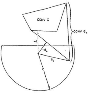
Figure 1.1: Constructing in Wolfe’s Method.

By using the following characterization of gradient:

v/(x) =

-iV r d f { x l

We can write V / ( x ) = —N r (conu{^,· : i € J(x)}) = —Nr {^,· : i G -f(x)}·

r.'ovv assuming that we have a bundle Gk — {gk-p, ■■■, 9k-i,gk] , (where p is a natural number less than k) we set dk = —N r Gk be the direction of steepest descent of / at

Xk-Wolfe [20] presented a conjugate subgradient method for minimizing non differen­ tiable functions, which is based on bundle methods with a special line search. Assuming that we have a bundle

x o y - , X k , g o ,...,g k , f { x o ) ,...- ,f { x k )

the algorithm works as:

i) Compute dk = —Nr Gk where Gk = {po, · · · ,gk}·

ii) Line search gives t > 0, and gk+i € d f ( x -b tdk}·

iii) Set

iv) If the optimality conditions are not satisfied, go to (i), else stop.

Computing G+,d+ (G+ = Gk+i, d = dk, d+ = dk+i) is shown geometrically in Figure 1.1.

If x q, . . . , X k axe close together, the above iteration continues until ||<ijt|| < e for some

k = K and then if

^ Ifxjt+i -Sfcll < 6 k<K

is satisfied, the optimality conditions can be checked, if not, a reset step is begun.

Resetting is done by choosing Gk = {fiffc}, that is by discarding all the previous subgradients. Wolfe’s algorithm constitutes an extension of the method of conjugate gradients method of Hestenes and Stiefel [11].

2. A N E W C O N JU G ATE G R A D IE N T

A P P R O A C H FOR N O N -S M O O T H

O P T IM IZA T IO N

We consider the feasibility problem :

Po s.t. Ax < b

X > 0

where A G x G 7?.” , b G and A is not necessarily full raw rank. Problem Pq

is equivalent to:

s.t. Ax = b

X > 0

where A = A \ L · e 7г'" X 6 7?.’” +” .

by adding the slack variables and identity to A we have nonsingular matrix Q as:

( dll Q = dml ■ · · 1 0

0

^Im 1 0

0 ^

0

I I

0

^ m n

0 ... 0 1

0 0 ...

0

0 ;

1 0 ... ... oj

V 0 (

Then A = Q^Q is a positive definite matrix and we make the transformation:

b = Q^b*

Where we define b* as:

b* =

and where b* , i = 1,2, . . . , n are choosen as:

h-m

It is known that if we drop the non-negativity constraints, then it is possible to solve the system of Ax = 6 by conjugate gradient method which terminates in k iterations such that k < n + m (here A 6 7^(n+m)x(n+m)^ gy conjugate directions we mean A-conjugate or A-orthogonal directions, so:

diAdj = 0 i ^ j \/i,j

dfAdi ^ 0 Vi

In fact since A is positive definite, then: d{Adi > 0 Vi . As mentioned in section 2.5 Wolfe’s algorithm constitutes an extension of the method of conjugate gradients method of Hestenes and Stiefel. Based on this we will introduce a set of A-conjugate directions

{di}^=i^ and perform search on these directions successively. Whenever it is necessary

we will compute the conjugate directions by Gram Schmit orthogonalization process.

For the feasibility problem Pq we define the penalty function Fi(x) aa follows:

m n+m

= ¿ ( a . ® - b if + ^ [min(0, 0:^)]^

t = l i = l

Recalling that A = Q^Q and b = Q^b* , we drop the non-negativity constraints and solve the system of Ax = b. Assume that we have found the conjugate directions

{d i},i = 1, . . . , n -f m and let the step sizes in any direction di, be a,·, z = 1, . . , n -|- m. then we can write the solution as;

X — X Oiid\ -|- . . . -f- Oin+mdn+m

where x'^ is any arbitrary starting point. Solving the system of Ax = b is equivalent to minimizing the:

F(a:) = [Ax - 6]*[Ax - 6]

Starting from rc° then the step size in direction dk would be ajt

F{x°) = [Ax° - bf[Ax^ - b]

F(x^) = [A(x° + akdk) — bY[A{x^ + akdk) - 6]

d F { x ^ )

d a k = 0 2{AdkY\A{x^ + akAdk) — 6] = 0

{AdkYAx^ + ak{Adk)^(Adk) - {Adk^b = 0 (Adk)^b — (Adk)^ Ax°

\ A ^ l

a k =

( d k f A F b - (d k fA ^ A x^ {dkYATAdk

Here ak is the optimal step length in direction dk without considering the non-negativity constraints and let a = iQi«!·

Assume we have 6* ,i = l ,2, . . . , n such that the unique solution of Qx — b* is a feasible solution to Po and let the set of A-conjugate are given, if we use the optimal step sizes , we have:

E i=l n-f m Oi ( -f ^ ajdj ) - 6,· j=l - I 2 = 0

since X = -f ajdj is a solution.

Now consider using step sizes dj , i = 1, 2 , . . . , (n + m ) rather than o,· , i = 1 , 2 , . . . , (n-f m) and we choose 6 as:

^ = m jn | | ^ l :

then we have the relative reduction:

E ”JT (g.-^° - - E r ir |ii (x ° + ^ <^a ) -f · ;'

E ”i r (<jix» - i ; f

That means if we define error at x^ as

n+m

= 2 9- 9"^

A* = E

- i-:).

1=1

then we have

Since A < 2^ ( here L is the size of the system of linear equalities ) then we can stop after ¡3 iterations for which

2 ^ { i - 2 0 + e-‘ Y

Which means we can bound the number of iterations as - 2L lo g2

log (1 - 2^ + 0^)

This definitely implies a polynomial bound for for problem Pq for any 1 > ^ > 0. In

this work we could not prove the existence of such 6 , but the computations results in the next chapter seems to support this idea that practically our algorithm can solve problems in polynomial time bound. It means that if in any loop the improvement in any direction is not posssible, we can remove that direction from the set of conjugate directions and the procedure reduces to search in the directions remained in the bundle of directions, and then it is possible to find a 0 < 0 < 1 , such that we can improve in all remaining directions.

i) Choose X® in 72·"·*·”* , the starting point, and sufficiently small e, 5 > 0, A = 0.

ii) Compute the conjugate gradient directions {d ,}, i = 1 , . . . , n + m by the method of C.G. algorithm and normalize them.

iii) For i = 1 to n + m do

de = di, do line search, = a; + tdi

X = X + \t\

if Fi(x·*·) < £ then stop, a feasible solution is found, else check the optimality test, if x"*· is optimal, then stop, end (For).

if min < 6 then (Reset) go to step (iu). else set A = 0 and repeat step (Hi).

iv) Set vi = — VFi(x·*·) , choose V2,...,Vn+m such that vi,V2, . . . ,Vn+m are inde­

pendent.

v) Find conjugate directions {d,·}, i = 1,2, . . . , n + m by the procedure of C.G.Schmit, normalize them, set A = 0 and go to step (iii).

The Main Algorithm:

C o n v e rg e n ce R esu lts:

D efin ition : Let W be the set of minimum points of F i(x) and let VF 7^ 0 . A sequence in 72" is called strictly Fejer-Monotone with respect to the set W , if for every x G FF we have:

\xfc+i — x|| < llx^' — x|| for all A: > 1

Every Fejer-Monotone sequence is bounded if FF 7^ 0 , since ||x^' —x|| is always positive and monotonically decreasing with FF [23].

D efin ition : Let {d,}"J"/" be A-conjugate directions such that di = —y/(x*') and d2,da,. . . ydn+m are generated by C.G. or C.G.S. algorithms with respect to di and a positive definite matrix A. We say a loop k is processed if starting from point , a set of line searches are done on all directions of the set {d. jfj"]”* and we reach the new point x*·*·*^. Of course this process is equivalent to n + m iterations.

T h e o re m 1 (basic idea due to Shor[17j) let F be a convex function and VF 7^ 0 ,

then any sequence generated by the algorithm above is strictly Fejer-Monotone

with respect to W and for any £ > 0 and any x* ^ W there exists a k and x such that F ( x ) = F (x^) and:

Where h is a real positive number.

Proof: Without loss of generality assume that in any loop the directions

are not suitable for improvement in line searchs. Then our algorithm reduces to a subgradient type method, that in any loop we have:

where: /ifc+i = steplength

„k „2

let X* e W ||x*+^ - x*|| = llx'' - X * - hfc+iijpf||||

~ | | x ^ —

X

II +

—

2 / i t 4 . x < x *^ —

X*,

>

if = 0 then X = X*’ = X*.

So let g'^ ^ 0 and take ik = < x^ — x*, > which is distance from x* to the hyperplane: fTx: = {x : < , x*' — X > = 0} Define D , = { x : F (x ) = F{x'‘ )} bk(x*) = min ||x* — x|| x€Dk

Since Dk and x ‘ are in one side of Hk , then any segment joining the point x* to a point

oi Hk passes through Dk- so we have :

4(.T*) > bk(x*)

||x^+i _ a;*||^ < lla;''· _ a:*||^ + - 2hk+ibk{x*)

let h be sufficiently small positive number as a constant stepsize:

||o;^+i _ a;*||2 < ||a;'= - a:*||'* + /i" - 2hbk{x*)

now if bk(x*) < 1 for all

A:

= 1,

2

. ..

||x^+^ — x*||^ < ||x*^ — x*||^ — eh^ < ||x^' — x*||^ — e (l + k)h'^

But since ||x*·*·^ — x*|| > 0 then there exists k such that:

hi^*) = min ||x* - x|| < ^(1 + e)

so no matter how small e or h is, we can find a k such that is the minimizer of

jP(x) and

II®

Optimality Conditions:

Ben-Tal and Zowe [2] derived the necessary and sufficient optimality conditions for the exterior penalty function:

1 ^

P e m in f(x ) = ho(x) -f -/9 ^ [m a x {0 ,/i,(x )}]^ .

^ t = l

First, it is convenient to define the following index sets:

E -- {¿1 = 0}

E+ = {i| hi(x~) > 0}

Theorem 2 Necessary and sufficient, optimality conditions for problem P«

(a) A necessary condition for x* to be a local minimizer of problem Pg is that

K(^‘)

+ E

=

0

i&E+

and for every d € 7^”+”^,

ho(x) < d , d > -f-p ^ hi{x*)h” { x ’') < d , d > -f p ]^[max{0,/i'(x*)d}]^

ieE+ i&E

+P > 0.

i€E+

(b) A sufficient condition for x* to be an isolated local minimizer for problem Pg is as above but with strict inequality for d ^ 0.

For our penalty function we have:

p = 2

s = n -f m

hi(x) = —x,(the negative of the element of x)

and

ho(x) = - h if

1=1

O p tim a lity Test: We have a set of conjugate directions D = , then a point

X* is an optimal solution of F i{x) if sufficiency condition of optimality is satisfied for

any dk and —dk such that dk E D, = 1 , 2 , . . . , n + m. Since any set of conjugate directions are also independent, then any arbitrary direction de can be written as the linear combination of the elements of the set D , that is d^ = rk E TZ. and dk E D.

So if sufficient conditions for optimality at a point x* is satisfied for any dk and —dk such that dk €: D, ^ = 1,2, . . . , n + , then it will be satisfied for any dg G and in this way the existing point x* will be optimal solution.

Of course the optimality test is not necessary for feasible problems and for the attempt feasibility problems we never used this test (for feasible problems), because min Pi (x*) = 0 for a feasible point x*. But in application of our algorithm for LP problems we need to use this optimality test.

3. NUMERICAL EXPERIMENTATION

We decided that for our A-conjugate method, we need to check the effectiveness of the algorithm practically. So we generated a series of random problems in different sizes and applied our algorithm to solve them. In these problems, that we give in tabular form in this chapter, the size of A changes from to , and for larger problems we need to modify the C.G. algorithm to find exact A-conjugate directions.

Recalling from the last chapter, although we could not guaranty the existence of

0 < 0 < 1 in any loop of iterations ( n+m iterations ) to support the polynomiality motivation of our algorithm, but as it is seen from the computations results in this chapter, the method solves problems in polynomial time bound practically at least for the size range of problems given above.

Due to numerical errors the accuracy of search directions ( generated by C.G. or C.G.S. processes) to be A-conjugate is decreased as size of A increases. The sparsity of the matrix A for all the solved problems is over 80 percent (that is the number of non-zero elements of A is more than 80 percent of its all elements) besides there is not any conditions on A and b.

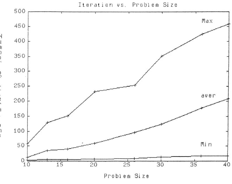
The important result from numerical experimentations is that, for all solved prob­ lems the convergence is so quick in first loop, that is for the problem of size 7^” *^" the penalty function is reduced exponencially at first n iterations and reachs to a relatively very small penalty value with respect to its initial value and then the process achieves a rather slow convergence. The worst case of number of iterations necessary to find a minimizer of penalty function in our test, is bounded by 15n.

Since the symmetric and positive matrix A may be ill conditioned, for example some of its eigenvalues may be too small, then in calculating A-conjugate directions the roundoff errors may be too large and this leads to the cases where d\Adj ^ 0 for

1 ^ j , so the set can not exactly represent 7^"+”* space.

FACTORS 1C = 10 /C = 13 x: = 16 IC = 20 1C = 26 1C = 30 1C = 36 !C = A0 m n Uij hi NZ UCj Icj pc 4 6 20 -20 4 10 - 1 0.8 5 8 20 -20 5 10 - 1 0.8

6

10 20 -20 6 10 - 1 0.8 8 12 20 -20 6 10 - 1 0.8 10 16 20 -20 8 10

- 1

0.8 12 18 20 -20 8 10 - 1 0.8 16 20 20 -20 12 10 - 1 0.8 16 24 20 -20 12 10 -1 0.8 Table 3.1: Schedule of design of test problems

K, = m =

n = Uij

"ij

dimension of the space, A G number of linear inequalities.

number of variables without adding slack variables, upper bound for d,j.

lower bound for d,_,·.

UCj =

Icj =

upper bound for Cj.

lower bound for Cj.

N Z = number of non-zero elements in every column

density of number of non-zero elements of c.

total (relative) step length during one loop (m -|- n iterations).

Pc =

A _

problem # ^ of iterations _{/( * )} min ( ¿ ) average 1 3 0.003860 0.017921 0.017921 2 4 0.007682 0.004227 0.004227 3 3 0.000367 0.004419 0.004419 4 3 0.007072 0.011708 0.011708 5 17 0.000874 0.003076 0.004755 6 28 0.010914 0.005772 0.012161 7 3 0.001199 0.003783 0.003783 8 3 0.001846 0.004212 0.004212 9 3 0.000119 0.001505 0.001505 10 3 0.000819 0.002757 0.002757 11 56 0.010789 0.000249 0.019070 12 19 0.006049 0.000003 0.001483 13 26 0.016264 0.003028 0.014203 14 15 0.016651 0.002718 0.007129 Table 3.2: Ax = b , A G

problem # ^ of iterations _f(^) min (A) average

1 5 0.000922 0.004142 0.004142 2 5 0.013952 0.002545 0.002545 3 20 0.003806 0.001378 0.002427 4 5 0.000570 0.009462 0.009462 5 30 0.019781 0.000052 0.006128 6 32 0.019084 0.000030 0.003567 7 5 0.010253 0.005145 0.005145 8 41 0.016802 0.000012 0.002100 9 72 0.019898 0.000094 0.010462 10 129 0.019927 0.001547 0.009797 Table 3.3: Ax = b , A e

20

problem ^ of iterations _f(^) average 1 23 0.002494 0.000200 0.001460 2 6 0.001620 0.011088 0.011088 3 58 0.017985 0.000874 0.010186 4 54 0.009547 0.000021 0.021087 5 39 0.018295 0.000102 0.002721 6 6 0.000240 0.015218 0.015218 7 72 0.018383 0.000108 0.007236 8 6 0.000549 0.004565 0.004565 9 7 0.002867 0.009162 0.009162 10 62 0.014058 0.000364 0.010775 11 59 0.014058 0.000221 0.005854 12 87 0.015753 0.000100 0.008568 13 5 0.008931 0.002479 0.002479 14 6 0.000389 0.007353 0.007353 15 16 0.016699 0.037585 0.037585 16 6 0.000414 0.007798 0.007798 17 54 0.014726 0.000047 0.018080 18 77 0.019968 0.000305 0.009002 19 72 0.015961 0.000092 0.007809 20 151 0.019186 0.000248 0.004713 Table 3.4: A.T = 6 , A € 21

problem # of iterations _f(^) min (A) average 1 53 0.007171 0.002620 0.006169 2 55 0.015347 0.005015 0.007598 3 7 0.007326 0.004334 0.004334 4 9 0.006160 0.013377 0.013377 5 52 0.011085 0.000143 0.026794 6 28 0.007784 0.000488 0.001557 7 25 0.019862 0.000031 0.040541 8 112 0.019612 0.000012 0.039558 9 9 0.005295 0.014534 0.014534 10 29 0.019185 0.000306 0.017977 11 10 0.018377 0.026277 0.026277 12 50 0.008287 0.000080 0.014182 13 49 0.017067 0.000080 0.010122 14 73 0.013925 0.001308 0.010502 15 69 0.019215 0.000271 0.011067 16 74 0.013281 0.000848 0.020566 17 75 0.018330 0.000522 0.008848 18 231 0.018757 0.000734 0.002817 19 76 0.009882 0.000732 0.006515 20 56 0.014150 0.005013 0.009095 21 115 0.019891 0.000747 0.006236 Table 3.5: Ax = b , A G 22

problem :fl: of iterations _f(^) min (^ ) average 1 19 0.012911 0.029228 0.029228 2 191 0.029996 0.000006 0.004158 3 36 0.027740 0.000320 0.018018 4 67 0.007212 0.000330 0.005650 5 11 0.015245 0.005242 0.005242 6 144 0.029670 0.000050 0.005359 7 10 0.007677 0.006737 0.006737 8 149 0.029920 0.000382 0.100395 9 64 0.012921 0.000136 0.004630 10 9 0.010766 0.022777 0.022777 11 68 0.027688 0.000161 0.004136 12 149 0.029920 0.000382 0.100395 13 64 0.012921 0.000136 0.004630 14 9 0.010766 0.022777 0.022777 15 68 0.027688 0.000161 0.004136 16 70 0.024106 0.002148 0.007798 17 169 0.029791 0.000020 0.010201 18 173 0.026735 0.000071 0.001617 19 64 0.026865 0.000230 0.015913 20 91 0.026094 0.000119 0.004617 21 95 0.013781 0.000310 0.006535 22 89 0.027748 0.000033 0.004375 23 143 0.023141 0.001590 0.005584 24 253 0.018113 0.002862 0.068871 Table 3.6; Ax = b , A e 23

problem # # of iterations _f(^) mm

_{H U}

average

_M

1 2 3 4 5 6 7 8 9 10 11 12 13 14 14 106 134 14 80 103 200 111 225 102 352 75 104 104 0.008159 0.028005 0.024513 0.011539 0.024698 0.016989 0.027437 0.010574 0.029625 0.026161 0.029524 0.021587 0.029698 0.029981 0.081600 0.000065 0.000022 0.007543 0.001907 0.000051 0.002198 0.001337 0.000014 0.000006 0.000163 0.000295 0.000009 0.000031 0.081600 0.006770 0.004174 0.007543 0.019771 0.018905 0.055168 0.007677 0.001667 0.003876 0.002316 0.012395 0.004808 0.007279 Table 3.7; Ax = b , A e

problem # of iterations _fi^) average (^ )

1 196 0.028532 0.000001 0.045340 2 273 0.026510 0.000483 0.014159 3 51 0.028544 0.004593 0.123871 4 17 0.026963 0.208405 0.208405 5 47 0.023672 0.001274 0.066795 6 235 0.021095 0.000081 0.180527 7 425 0.029967 0.000001 0.197356 Table 3.8: Ax = b , A e

problem # ^ of iterations _f{^) min (^) average j

1 143 0.028990 0.000039 0.092190 2 458 0.013592 0.000677 0.132495 3 62 0.028406 0.004004 0.048863 4 185 0.029546 0.000174 0.019071 5 17 0.026838 0.014640 0.014640 6 138 0.022210 0.000061 0.038515 7 176 0.028839 0.021943 0.540074 8 386 0.028450 0.000309 0.003927 9 318 0.029407 0.000971 0.018176 Table 3.9: Ax = b , A e 24

i: t. (·) I' a t. io n VO. P I' 0

1

;)

1

o m Si z e

hi u

in

t) « 0 f i; t 0 r'

a

t.

i

0 n

Figure 3.1: Number of Iterations vs. Problem Size

4. A P P L IC A TIO N S

4.1

Linear Inequality Models in Computerized Tomography

Computerized tomography [23} is a method in which the image of the cross section of the body is reconstructed by a computer. It can be used to show a three dimensional view of the interior structures of the human body and so CT can detect some conditions that conventional X-ray pictures can not detect. Initially the structure ( which can be brain, heart, etc.)which is being studied, is divided into slices and then as finite element method any slice is considered to be divided into sufficiently small pixels. The process for a two dimensional slice is as follows:

An X-ray beam, say beam 1 penetrate the slice, entering it with the initial intensity Ji, and emerges at the detector at the end of its path through the slice, with an intensity

Fi- Hence the total absorption of the energy through the path is F — Fi. Define a-ij

be the length of the intersetion of the path of beam number 1 with the pixel, and say Xj be the unknown local density of the pixel and assume the data is collected from m different beams for every slice, then we have:

O'ijXj — hj i — 1 , 2 , . . . ,

i=i

n

where hj = Ij — Fj

Since the assumption that the local density is a constant within each pixel, is unlikely to be valid and since the local densities are not negative, so we can replace upper system by the inequality system as:

i>i

- £.· <

X ] CLijXj < b{

-f £,·

j=i

1 < f < ?n

0 < .T,· < u 1 < i <

where u is a known upper bound for the density of pixels and n equals to the total number of pixels in slice. Solution of this system of linear inequalities gives densities of the object under study.

4.2

L IN E A R P R O G R A M M IN G V I A N O N -SM O O T;ri O P T I­

M IZ A T IO N

In this chapter we try to extend our algorithm for solving the linear feasibility problems to solve linear programming problems. We onsider the LP problem :

P i

where A 6 7?.'"^", c and x G 7^" , b G 7Z”

Adding slack variables we have :

max cx s.t. A x < b x > 0 max cx s.t. Ax = b X > 0

where A = A I Im] e and .t G 7г^+".

There are alternative ways of reducing this LP to a feasibility problem, one way, which we have tried is the following: Recalling the exterior penalty function

1 ^ m in /(x ) = /io(x) + -p ^ [m a x {0 ,/i,(a ;)}]P , p > 1 «=1 where: < s P . hi(x) a natural number, a positive real number.

smooth function defined on a real normed vector space.

We define the exterior penalty function F2{x) for the LP problem P i as:

m n-f-m

F2{x) = {cx - K f + ¿ ( a , x - bif + £ [min(0, Xj)^

t = l 3= 1

Here K is an upper bound for cx and we assumed that p (the penalty weight) equals 2 for any penalty term, and

ho{x) = {cx - K Y + ^{b-iX - b if i=l

hi{x) = —Xi (the negative of the element of x )

i) Choose in the starting point, and p > 0, A = 0.

ii) Compute the conjugate gradient directions {di},i = 1, .. . ,n + m. by the method of conjugate gradient of Hestenes and normalize them.

hi) For z = 1 to n 4- nr do

d( = di, do line search, = x + td(

A = A + |i|

Check the optimality conditions, if is optimal solution, then stop, end (For).

if F i(x+ ) < e then go to step(uz).

if min(A, A) < S, then (Reset) go to step (zu), else set A = 0 and repeat step (zzz).

iv) Set ui = —VFi(a;·^), choose V2, .. . ,Vn+m such that V\,V2, ■.. ,Vn+m are indepen­

dent.

v) Find conjugate directions {d ,}, z = 1 , 2 , . . . , n -f m by the procedure of C .G .S . , normalize them, set A = 0 and go to step (zzz).

vi) Improve c.t by the following procedure (it needs n iterations):

The Basic Algorithm;

consider the simplex tablaue:

^ Cl C2 c„ 0 .... 0 '

dll di2 din 1

U7712 · '' · ^mn ₀

Given X then for z = 1 to n set the lower bounds as:

Xi

>

0

£i =

0

Xi <

0

= Xi

and for z = ?r -f- 1 to n -4 m set the lower bounds as:

Xi >

0

= 4

£i =

0

Xi < 0 ==4 A’ = Xi — P

Cj = Cj — TTO·'

Cj = Cj — c bB = Cj — CB<P

C ase 1:

if Cj > Ojg// — ^ ■* ^

if Ji < 0 Vi then problem is unbounded, else we find $ such that:

$

=

$i,

= min|^^‘_^.

> o|

hence Xj enters the basis and .t,·. leaves the basis.

Case 2:

if Cj < — r' Xj * Xj ~ Q

xb — xb -{■

Where 9 = min 9x, $2 and 9i = Xj — Ij and

92 = 9i. = min | - - d\ < o|

If 0 = 9·^ then nonbasic j reachs its lower bound and basic doesn’t change. If

9 — 92 then Xi· leaves the basis and Xj enters the basis.

vii) Go to step (iu).

We randomly generated some LP problems and solved those by our algorithm but the results show that the method is not efficient for solving LP problems by using the exterior penalty function F2(x). We have also tried primal and dual problems together, but the results do not seem promising.

problem ^ solution by Undo solution via NSO 1 99.179 99.184 2 unbounded unbounded 3 395.34 369.70 4 72.135 68.30 5 85.71 80.30 6 260.00 260.41 7 123.179 118.73 8 109.434 109.45 9 132.699 132.71 10 70.339 69.667 11 70.87 69.174 12 83.849 83.853 13 198.860 171.08 Table 4.1: Ax = b , A e

problem # solution by Undo solution via NSO

1 246.420 245.00 2 88.958 89.17 3 231.291 231.558 4 50.216 50.66 Table 4.2: Ax = b , A G

30

5. CO N CLU SIO N S

For the feasibility problem, our non-smooth approach seems to be more efficient, at least in the size range of computations discussed in chapter 4 . In the surrogate con­ straint methods which are efficient versions of relaxation methods, there is no measure of usefulness of the selected surrogate constraint. As a future work, we consider using our algorithm together with the surrogate constraint methods. In our algorithm the penalty function is reduced exponentially in the first loop of iterations ( the first n-|-m iterations ). So implementing our algorithm in the beginning of the surrogate constraint method will probably yield more efficient results.

In the case of implementing our algorithm for L P problems we see that putting the objective function as a penalty term in the so defined non-smooth penalty function has a detrimental effect on the convergence of the algorithm. We worked on some variants of penalty functions to decrease that effect of the objective function by assigning a small penalty weight, but it seems that for LP case the penalty weights must be arranged in a more suitable way to gain an effective algorithm.

B IB L IO G R A P H Y

REFEREN CES

[1] Agmon S., ” The relaxation method for linear inequalities ” , Canadian Journal of

Mathemaiics 6 (1954), 382-392.

[2] Ben-Tal A. and Zowe J., ” Necessary and sufficient optimality conditions for a class of nonsmooth minimization problems ” , Mathematical Programming 24 (1982), 70- 91.

[3] Burke V., ” Second order necessary and sufficient conitions for convex composite NDO ” , Mathematical Programming 38 (1987) 287-302.

[4] Coleman T.F. and Conn A.R., ” Nonlinear programming via an exact penalty function: Global Analysis ” , Dept, of Computer Science Tech, report CS-80-31, July, 1980, University of Waterloo.

[5] Coleman T.F. and Conn A.R., ” Second order conditions for an exact penalty function ” , Mathematical Programming 19 (1980) 178-185.

[6] Conn A.R., ” Constrained optimization using a nondifferentiable penalty function ” ,SIAM J. Numer. Anal. vol. 10, No. 4, September 1973.

[7] Conn A.R., ” Linear programming via a nondifferentiable penalty function ” , SIAM

J. Numer. Anal. vol. 13, No. 1, March 1976.

[8] Conn A.R. and Pietrzykowski T., ” A penalty function method converging directly to a constrained oi^timum ”

,

SIAM J. Numer. Anal. vol. 14, No. 2, April 1977.

[9] Fletcher R., ” Practical methods of optimization ” , John Wiley , Great Britain 1987.

[10] Goffin J.L., ” The relaxion method for solving systems of linear inequalities ” ,

Mathematics of Operational Research , vol. 5, No. 3, August 1980.

[11] Hestenes M.R., ” Conjugate direction methods in optimization ” , Spinger-Verlag, New York 1985.

[12] Himmelblau D.M., ” Applied nonlinear programming ” , McGraw-Hill, New York 1972.

[13] Lemarechal C. and Mifflin R.(Eds), ” Nonsmooth optimizitation ” , IIASA Pro­

ceedings S, Pergamon, Oxford 1977.

[14] Motzkin T.S. and Schoenberg I.T., ” The relaxation method for linear inequalities ”

,

Canadian Journal of Mathematics 6 (1954), 393-404.

[15] O ’Neill P.F. and Conn A.R., ” Nondifferentiable optimization and worse ” , Deg.

of Combinatorics and Optimization report CS-83-05, March 1983.

[16] Polak E. and Mayne D.Q., ” Algorithm models for nondifferentiable optimization

” ,

SIAM J. Control and Optimization vol. 23, No. 3, May 1985.

[17] Shor N.Z., ” Minimization methods for nondifferentiable optimizationy ” , Springer-

VerlagBerlin, Heidelberg 1985.

[18] Shrijver A. and Grotschel M. and Lovasz L., ” Geometric algorithms and combi­ natorial optimization ”

,

Springer-Verlag Berlin, Heidelberg 1988.

[19] Teigen J., ” On relaxation methods for systems of linear inequalities ” , European

Journal of Operational Research 9 (1982) 184-189.

[20] Wolfe P., ” A method of conjugate subgradients for minimizing nondifferentiable functions ” , Mathematical Programming Study (1975) 145-173.

[21] Womersley R.S., ” Local properties of algorithms for minimizing nonsmooth com­ posite functions ”

,

Mathematical Programming 32 (1985) 69-89.

[22] Wright S.J., ” Local properties of inexact methods for minimizing nonsmooth com­ posite functions ”

,

Mathematical Programming 37 (1987) 232-252.

[23] Yang K. and Murty K.G., ” Surrogate constraint methods for linear inequalities ” ,

Department of Industrial and Operations Eng. University of Michigan, June, 1990.