FOREIGN TRADE AND NINETEENTH CENTURY AMERICAN
GROWTH
*Doç. Dr. M. Erdem Özgür Prof. Dr. Hasan Vergil Dokuz Eylül Üniversitesi İstanbul Üniversitesi
İşletme Fakültesi İktisat Fakültesi ORCID: 0000-0002-0324-011X ORCID: 0000-0001-9629-3036
● ● ●
Abstract
The American economy exhibited an impressive growth in the nineteenth century. There certainly are numerous factors at play in this extraordinary growth story. This paper presents a quantitative analysis which investigates the role of foreign trade in the nineteenth century American growth. To this purpose, the relationship between real exports, real imports and real GDP is questioned between the years 1820 and 1910. Since the American Civil War was an extremely important event in the American history we divided the period under examination into two, 1820-1860 and 1867-1910 periods. By examining causal relationship, we aim at investigating the existence of export led growth, growth led exports, import led growth and growth led imports hypotheses during the periods before and after the Civil War. While the results exhibit a strong evidence for growth-led imports in both samples, export led growth, growth led exports and import led growth hypotheses are supported only in the second period.
Keywords: US, Nineteenth Century, Foreign Trade, Economic Growth, Causality
Dış Ticaret ve Amerikan Ekonomisinin Ondokuzuncu Yüzyıldaki Büyümesi
Öz
Amerikan ekonomisi ondokuzuncu yüzyılda çarpıcı bir büyüme sergilemiştir. Bu sıradışı büyüme hikayesinin arkasında mutlaka farklı etkenler vardır. Bu çalışma Amerikan ekonomisinin ondokuzuncu yüzyıldaki büyümesinde dış ticaretin etkisini araştıran niceliksel bir çalışmadır. Bu amaçla 1820 ve 1910 yılları arasında reel ihracat, reel ithalat ve reel GSYİH arasındaki ilişki sorgulanmıştır. Amerikan İç Savaşı Amerika Birleşik Devletleri tarihinde çok önemli bir rol oynadığı için bu dönem 1820-1860 ve 1867-1910 olarak iki bölümde ele alınmıştır. Nedensellik ilişkisinin olup olmadığını belirlemek için Amerikan İç Savaşı öncesi ve sonrası dönemlerde ihracat yönlü büyüme, büyüme yönlü ihracat, ithalat yönlü büyüme ve büyüme yönlü ithalat hipotezlerinin varlığı incelenmektedir. Çalışmadan elde edilen sonuçlar büyüme yönlü ithalat hipotezinin her iki dönemde de geçerli olduğunu gösterirken, ihracat yönlü büyüme, büyüme yönlü ihracat ve ithalat yönlü büyüme hipotezlerinin sadece ikinci dönemde geçerli olduğu yönünde güçlü bulgular sunmaktadır.
Anahtar Sözcükler: ABD, Ondokuzuncu Yüzyıl, Dış Ticaret, Büyüme, Nedensellik
* Makale geliş tarihi: 18.07.2016 Makale kabul tarihi: 17.07.2017
Foreign Trade and Nineteenth Century
American Growth
Introduction
The nineteenth century American growth is impressive. An agricultural country with an economy based primarily on natural resources turned into the most developed country in the world before the Great War. There are countless accounts of this extraordinary story. Some of these accounts emphasized the role played by exports (North, 1961), such as cotton, and imports, some of them emphasized territorial expansion, natural resource abundance, population growth, accumulation of capital, institutional development, financial system, the power of entrepreneurial activity and increasing productivity (Rousseau and Sylla, 2005; Tuttle and Perry, 1970; Kravis, 1972; Davis, Easterlin and Parker, 1972; Ratner, Soltow and Sylla, 1979; Landes, 1999; Acemoglu, 2012). There is no doubt that all of the above factors contributed to American growth and it is not meaningful to single one of them out as the only source of growth. In this paper, a quantitative analysis which investigates the role of foreign trade in the nineteenth century American growth is presented. To this end, the relationship between real exports, real imports and real GDP is questioned between the years 1820 and 1910. To the best knowledge of the authors of this work, an econometric analysis which specifically targeted the role of exports and imports throughout the nineteenth century American growth and causality relationships among them are not available in the American economic history literature. (Vergil and Özgür, 2013) which is covering a different time period and which has a narrower scope, questioned the existence of an export-led growth in the US during the Napoleonic Wars, reaching a conclusion that there was not, with reservations concerning the available data.
Since the American Civil War, fought between 1861 and 1865, was an extremely important event, we divided the period under examination into two, and we compared them. These are 1820-1860 and 1867-1910 periods. By doing this, we believe that we can show the differences between the effects of foreign trade on growth during these two periods, if there are any significant ones. These periods were certainly very different from each other in many ways, but
the scope of this study cannot be broad enough to inquire all the aspects of American economy during the period in question.
Since the main question of this study is the effect of trade on growth, one should focus on cotton exports of the US, since cotton exports were certainly an important revenue source for the US economy in the antebellum period. According to O’Sullivan and Keuchel (1989: 52), cotton constituted about one-half of the value of America’s exports by the early 1840s. Douglass North assigns an essential role to the export of cotton in explaining American growth before 1860. To North, the stimulant for the American antebellum growth was British demand1 for American cotton, which was the main input of the engine,
the textile sector, of the Industrial Revolution. According to North (1961: 69), “the cotton trade remained an important influence upon the economy until 1860, but its role declined in relative importance after the boom and depression that followed 1839.” He (1961: 70) states that “in the expansive surges of 1815-1818 and 1832-1839 they [terms of trade] became very favorable, reflecting a rapid rise in the price of American exports. In these two periods, it was cotton that accounted for the rise and appeared to initiate the subsequent flow of capital in response to the increased profitability of opening up and developing new sources of supply of the export staple and western foodstuffs.” As Lipsey (2000: 728) puts it “North described the role of growth in foreign demand for cotton in leading to the westward expansion of cotton farming and, in its wake, more general expansions in settlement and cultivation.”
The size of the internal market, a product of territorial expansion and population growth is another crucial factor which requires emphasis. According to O’Sullivan and Keuchel (1989: 134) “the growth of the American economy in the nineteenth century can be traced in the movement from local to regional markets and then on to a national market. By 1900 this market was held together by a grid of railroad lines.” This enlargement of the market size represents regional economic interdependence which unified the people in different sections of the country into more articulate economic units with a high degree of geographical and industrial specialization and division of labor. Although the volume of foreign trade increased throughout the nineteenth century, “it never was as important a source of income nor did it support as many people as did domestic trade and commerce” (Tuttle and Perry, 1970: 211, 498). Similarly, Kravis (1972: 405) argued that the origins of growth in the nineteenth-century US were internal. US found its areas of comparative
1 Atack and Passell (1994: 136) state that the US supplied about 80 percent of the cotton used by the British cotton textile industry.
advantage through trade, however it was a supplementary factor not the engine of growth.
Two of the most critical factors of American economic development up to 1860 are a westward expansion and the growth of population. Throughout the years between 1820 and 1860, i.e. during the first period under investigation, the population of the US rose from 9.6 million to 31.4 million (Tuttle and Perry, 1970: 135). Gallman (2000: 51) states that “the march of population and economic activity to the west followed a sequence of land acquisitions2 and was coterminous with the construction of transportation,
communications, and financial networks that tied the expanding economy together.” “History arranged things well” according to Braudel (1995: 470), “it enabled the United States to expand from the Atlantic to the Pasific, almost without hindrance.”
The increase in input per capita and the rise in productivity are other sources of growth underlined by economists or historians (Abramowitz, 1989; Broadberry and Irwin, 2006; Atack, Bateman and Margo, 2008). Gallman (2000: 14) asserts that “in the nineteenth century, growth of US output was apparently dominated by the increase of supplies of factor inputs. The rates of change of these inputs, taken together, accounted for between about 82 and 85 percent of the growth rate of output; productivity change, of course, accounted for the residual, 15 to 18 percent. Productivity seems to have contributed more to the expansion of the economy after 1840 than before, but the contrast between the two periods is not great.” A different argument for American growth was put forward by Rousseau and Sylla (2005), who argued that as new technologies emerged the innovative and expanding financial system of the US provided debt and equity financing to businesses and government, and this was a powerful determinant of the early growth and modernization of the country.
This paper investigates the causal relationship between real exports, real imports and real GDP in American economic history before and after the American Civil War. By examining causal relationship, we are investigating the existence of export led growth, growth led exports, import led growth and growth led imports hypotheses during the periods before and after the Civil
2 “After the Louisiana Territory was added to the US in 1803, the second largest single acquisition of new lands was that of Texas in 1845...The largest addition to the continental US was the Mexican Cession of 1848 by which over 560.000 sq miles of territory were added...The ownership of the Oregon Territory was settled by treaty with England in 1846...It remained for the Gadsden Purchase in 1853 to round out the territorial limits of the continental US.” (Tuttle and Perry, 1970: 143-145).
War. Since the relationship between trade and economic growth is vastly discussed in the literature, this paper focuses on and discusses only the mechanisms and procedures in providing evidence for the validity of these hypotheses.3 To achieve this objective, the exports, imports, real exports and
GDP variables are used for cointegration and causality analyses employing Johansen’s method and error correction models. The rest of the paper is organized as follows. Section 2 presents a brief discussion on trade before and after the civil war. Section 3 presents the source of data and the evolution of exports and imports. Section 4 first discusses econometric methods and then presents the estimation results. Section 5 summarizes and concludes the paper’s findings.
1. Trade Before and After The Civil War: An
Overview
Lipsey (2000: 700) argues that the United States was mainly an exporter of raw materials and foods before the Civil War. Raw materials alone constituted 60 percent or more of exports, “food exports were about 20-25 percent, and semi-manufactures and finished manufactures accounted for the rest, with the finished goods rising in importance and the semi-manufactures declining”. The period after the Civil War, however, saw very different trends. He (2000: 700) adds that “the share of raw materials fell to around 30 percent and food exports increased to replace them, reaching a peak importance of over 40-45 percent in the last two decades of the nineteenth century and then declining to about a quarter just before World War I.” According to Fite and Reese (1973: 222) “the political independence of the United States did not mean economic independence. The unfavorable balance of trade, the importation of manufactured goods, the exportation of raw materials, and the heavy reliance on foreign investment all indicate a continuation of a colonial type of economy. By the end of the period [1790-1865], however, the declining importance of foreign trade and the development of manufacturing signaled the beginning of the independent economy which the United States was to develop during the years after the Civil War.” Bensel (2000: 4) states that “industrialization transformed the United States from an agricultural, commodity-exporting dependency of Great Britain into an independent, leading force in the international system.” The leading exports of the US before the
3 Acemoglu (2009: 648-691) documents the large literature on trade and economic growth in a number of important aspects. For empirical papers, among others, see Marin (1992) and Awokuse (2006).
Civil War were raw materials (raw cotton, tobacco, livestock, wool, hemp), manufactures, manufactured foodstuffs; and the leading imports consisted of manufactures, crude foods and raw materials, and manufactured foodstuff (Tuttle and Perry, 1970: 235). In addition, a large volume of re-exports was an important feature of this period.
After the Civil War American economy experienced a rapid industrial expansion, but occurring in the Northeast and in the Midwestern states of Ohio, Indiana, Illinois, Wisconsin and Michigan, this expansion was extremely uneven (Bensel, 2000: 19). According to Lipsey (2000: 725), rapid growth in US manufacturing during this period involved import substitution. He (2000: 725) states that after the Civil War there was “a major shift in the balance of political power that was relevant to trade policy, since the southern states, more dependent on exports and more oriented to free trade, lost to the northern states, which were import dependent and more favorable to protectionist legislation.” He (2000: 725) adds that “the era after the Civil War is sometimes cited as a period in which the United States used high tariffs successfully to encourage infant industries that eventually became giants. In 1869 imports were 14 percent of the consumption of manufactured goods, and by 1909 that ratio had fallen to 6 percent.” According to Tuttle and Perry (1970: 248, 249) “as an agricultural section of the country and one that exported most of its money crop, the South was not interested in a tariff policy, except in a negative manner. The Northern and Middle Atlantic States were in favor of high protective tariffs in order to create and to protect infant industries from competition in the sale of foreign manufactured goods.” Northern merchants, on the other hand, were interested in tariffs as a means of keeping foreign competition out of a lucrative southern market.” According to Chang (2002: 61), the US was the pioneer country in infant industry protection, and during the period between 1816 and 1945 she “had one of the highest average tariff rates on manufacturing imports in the world.” For Bensel (2000: 6) “three great developmental policies underpinned American industrialization in the late nineteenth century: the political construction of an unregulated national market, adherence to the international gold standard, and tariff protection for industry.” The leading exports of the US after the Civil War were raw cotton, leaf tobacco, coal, petroleum, grain, fruits and vegetables, lard, meats and prepared fruits, lumber, iron and steel plates, refined copper, wood and iron products, textiles and cigarettes. The leading imports consisted of raw silk, hides and skins, crude rubber, coffee, tea, tropical fruits and nuts, sugar, meat, wheat flour, copper in bars, wood pulp, woolens, cotton textiles and lace, newsprint, iron and steel products, and manufactured fur products (Tuttle and Perry, 1970: 499-501).
2. Data and The Evolution of Exports and Imports
The data used is annual data of real GDP, exports, imports and real exchange rate spanning from 1820 to 1910. Since the Civil War was fought from 1861 to 1865, we divide the sample into two parts as a period from 1820 to 1860 and from 1867 to 1910. Real GDP, exports and imports data were obtained from the website of Historical Statistics of the United States Millennial Edition Online, http://hsus.cambridge.org/HSUSWeb/toc/hsus Home.do. The real GDP variable is readily available on the website in 1996 million Dollars. Nominal exports and imports data in million Dollars were converted to real terms by using the price deflator index of 1996=100. Furthermore, all series are transformed into natural logarithm form.
The number of US Dollars per British Pound is used as an exchange rate since the United Kingdom was the largest trade partner of the US during the time of the study. The nominal exchange rates are converted to real ones using
the formula of:
US UK P P Pound RER ) $ (
where PUK is the UK GDP Deflator
(index 2009=100) and PUS is the US GDP Deflator (index 2009=100). Increases
in real exchange rates correspond to cheaper US export goods. These data were obtained from Johnston and Williamson (2017) and transformed into natural logarithm form.
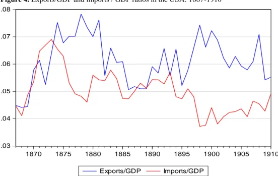
Before doing formal analyses, examining graphs of the variables might give a hint about causal flows among GDP, exports and imports. Even though correlation does not necessarily imply causality, correlation coefficients, 0.90 and above, indicate very high linear association among variables. Generally, the series follow a linear trend along the sample period. For the first sample period, the USA generally runs trade deficit, especially between 1830-1838 during which the country experienced acceleration in economic growth. Between the years 1842 and 1844, the imports declined more than exports and the USA had a trade surplus in these years (see Figure 2). For the period after the Civil War, starting from the 1874 the USA runs trade surplus for the rest of the period except the year 1888 (see Figure 3). The difference between the ratio of exports to GDP and imports to GDP had been very high during this period (see Figure 4).
Figure 1. Exports (in logs) , imports (in logs) and GDP (in logs) in the USA:
1820-1860
Figure 2. Exports/GDP and imports / GDP ratios in the USA: 1820-1860
6 7 8 9 10 11 12 1820 1825 1830 1835 1840 1845 1850 1855 1860 GDP Exports Imports .02 .03 .04 .05 .06 .07 .08 .09 .10 .11 20 25 30 35 40 45 50 55 60 exports/GDP imports/GDP
Figure 3. Exports (in logs) , imports (in logs) and GDP (in logs) in the USA: 1867-1910 8 9 10 11 12 13 14 1870 1875 1880 1885 1890 1895 1900 1905 1910 GDP Exports Imports
Figure 4. Exports/GDP and imports / GDP ratios in the USA: 1867-1910
.03 .04 .05 .06 .07 .08 1870 1875 1880 1885 1890 1895 1900 1905 1910 Exports/GDP Imports/GDP
3. Econometric Methods
3.1. Causality and Cointegration
If the current and future values of a time series are better predicted by using past values of another time series, then the latter is the cause of the former. This concept is provided by Granger (1969) and defined as xt fails to
Granger cause of yt if for all n > 0 the mean squared error of a forecast of yt+n
based on (yt, yt-1, yt-2,…) is the same as the mean squared error of a forecast of
yt+n based on (yt, yt-1, yt-2,…) and (xt, xt-1, xt-2,…). In the context of finite-order
vector autoregressive (VAR) models, while the short-run causality takes the form of relatively simple zero restrictions on the coefficients of the VAR at horizon one, long-run causality takes the form of zero restrictions on multilinear forms in the coefficients of the VAR at higher horizons (Dufoura et.al., 2006).
Testing for Granger Causality is straightforward. In the bivariate VAR model case with stationary variables of xt and yt, the Granger test is based on:
n i t m j j t j i t i t x y u y 0 1 1
(1)
n i t m j j t j i t i t x y u x 1 2 0
(2)where u1t and u2t are assumed to be uncorrelated white-noise error terms. The
test involves testing the null of “xt does not cause yt” by testing whether
i
0
for every i and testing the null of “yt does not cause xt” by testing whether
0
j
for every j. If there are more than two variables, the block Granger causality test should be used.
If the variables are not stationary either the models (1) and (2) might be estimated with variables in first differenced forms and similar tests might be performed or the models might be converted into the error correction mechanism (ECM) specification if the variables in the system are co-integrated.
Since the aim is to investigate the causal relationship between real exports, real imports and real GDP in American economic history before and after the American Civil War, we included real exchange variable in the system to control possible effects of restrictive trade policy such as tariff and non-tariff barriers which are directly related with other variables in the system. More specifically, if Y, X, ER and M denote real GDP (in logs), real exports (in logs), real exchange rate (in logs) and real imports (in logs) of the USA, respectively,
and assuming that these variables are not stationary but cointegrated, the following ECM models might be performed:
t t p m m t m p k k t k p j j t j p i i t i t b X c Y d M k ER e u Y 1 1 1 0 0 1 0 ˆ
(3) t t p m m t m p k k t k p j j t j p i i t i t f Y g X h M k ER e u X 2 1 2 0 0 1 0 ˆ
(4) t t p m m t m p k k t k p j j t j p i i t i t l X r M s Y k ER e u M 3 1 3 0 0 1 0 ˆ
(5) t t p m m t m p k k t k p j j t j p i i t i t l ER r Y s M k X e u ER 3 1 3 0 0 1 0 ˆ
(6)where
e
ˆ
t1in each equation is the OLS residuals obtained from the static long-run equilibrium regression:t t
t
P
e
Z
0
1
(7)where
Z
tis a (4 x 1) vector of variables in the system,P
tis a (3 x 1) vector of variables excluding the dependent variable,
0is a (4 x 1) vector of constant terms and 1is a (4 x3) matrix of parameters.Most important feature of the ECM is that a regression contains only stationary variables and reflects both long-run and short-run effects. Employing the coefficients in the equation 3, for example, while the short run causality is measured by testing the null “Yt is not caused by Xt”;H0:b1b2 ....bp 0
by the Wald test, the long run causality is measured by testing the null
0
:
0
H
.The existence of cointegrating relationship among a set of economic variables can be tested by residual based tests such as the methodology of Engle and Granger (1987) or Phillips and Ouliaris (1990). However, the single equation approaches cannot treat the possibility of more than one cointegration relationship in the case of more than two variables. The Johansen (1988) maximum-likelihood method, which is a very standard application in the literature, overcomes this problem and tests for the presence of multiple cointegrating vectors.
3.2. Unit Root Tests
Before testing for causality, we should examine stationary properties of the series by using unit root tests because the usual causality test for the level variables with possible unit root and cointegration in the VAR system could be misleading. Several unit root tests consider the form of
y
t
y
t1
t,where y is I(1), transform it into the auxiliary regression
y
t
(
1
)
y
t1
t and testfor
1
by using the t statistic, namely Dickey-Fuller tests (DF tests). Because the data generating process of the I(1) variable is unknown, an intercept and an intercept plus a time trend might be included in the original specification. However, while including too many of these deterministic regressors results in lost power, not including enough of them biases the test toward finding a unit root test. The other problematic issue with the DF tests is that the data generating process might have more than one lagged value of y on the right hand side. In this case, the auxiliary regression is amended to
yt
t (
1)yt1
i yti
t, namely the augmentedDickey-Fuller test (ADF tests) by Dickey and Dickey-Fuller (1979). Adding an appropriate number of lagged terms is also used to take account of any bias due to possibility of autocorrelated errors in the DF type regression models. Phillips and Perron (1988) use nonparametric methods to account for autocorrelation in error terms without adding lagged dependent variables.
While the ADF tests seem to be the most popular unit root tests, there are several problems with these tests regarding choosing incorrect form of the model, using inappropriate lag lengths and other several issues related to the size and power of unit root tests.4 Thus, researchers have devised new unit root
tests with better size and power properties. One of these tests, which is called Dickey Fuller Generalized Least Squares test (DF-GLS), is developed by Elliott, Rothenberg and Stock (1996) who propose a slight modification in the ADF test in which the power of the ADF test is optimized by de-trending of the series before running the regression. Under the null hypothesis of yt has a
random walk trend, possibly with drift, this test first estimates intercept and trend by generalized least squares such that
y
is regressed onz
which denotes a constant and time trend where;
4 There is a vast literature for issues and solutions to problems in unit root testing. For accessible discussions, see Maddala and Kim (1998: 98-154) and Harris and Sollis (2003: 41-76).
T
T z L z L z z y L y L y y ) 1 ( ,..., ) 1 ( , ) 1 ( ,..., ) 1 ( , 2 1 2 1
and)
,
1
(
t
z
t 1(c/T)where T is the number of observations and
c
is fixed at -7 in the model with drift and at -13.5 with the linear trend case. The estimators (bˆ0,bˆ1) arethen used to compute the de-trended yt series: y yt (bˆ0 bˆ1t).
d
t
In the second step, the regression
t d p t p d t d t d t a y a y a y u y
0 1 1 1 ... is estimated to test the null;
0
:
00
a
H
. Elliott et al. (1996) show that the Dickey Fuller t test applied to a de-trended series in this way has good power properties.In most of the unit root tests, the null hypothesis is that a time series under investigation has a unit root. Sometimes it is more convenient to have stationary as the null hypothesis since the unit root tests assuming a unit root in the series are biased toward finding a unit root unless there is strong evidence against it (Kennedy, 2003: 351). Kwiatkowski et al. (1992) have devised a test which adapts a null hypothesis of stationarity rather than the Dickey Fuller type null hypothesis of non-stationarity. The test can be performed with constant and constant and linear trend and can be used for confirmatory analysis for DF-GLS test.
Perron (1989) argued that the standard unit root tests, such as the ADF and DF-GLS tests, may not be reliable in the presence of structural breaks since they do not account for the possibility of a structural break. The tests without structural break will have low power and are biased toward finding a unit root. Thus, a unit root catching the structural breaks in a time series should be conducted to confirm the results of the previous tests. One of the commonly applied structural break unit root tests was developed by Zivot and Andrews (1992). This test allows for an endogenous determination of the date of the structural break. The break can be in the level of the series, in the slope of the trend function or both.5
5 Theoretical descriptions of the tests by Kwiatkowski et al. (1992) and Zivot and Andrews (1992) are skipped here since they are discussed thoroughly elsewhere such as by Maddala and Kim (1998) and Harris and Sollis (2003).
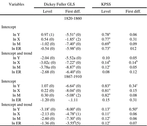
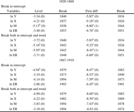
We measure stationary properties of the series in each time period with the methods of Dickey-Fuller GLS by Elliott et.al. (1996), KPSS test by Kwiatkowski et.al. (1992), and Zivot and Andrews (1992). Table 1 and Table 2 show results of these tests for two sample periods. The results of the Dickey-Fuller GLS and KPSS test mostly support the non-stationary of the variables in level and stationary in first differences. Similar conclusions are reached by the Zivot-Andrews test which considers the possibility of a structural break that series are mostly first difference stationary in two sample periods. Based on these tests, we conclude that all series are I(1). Thus we should check whether variables are cointegrated.
Table 1. DF-GLS and KPSS tests for unit roots
Variables Dickey Fuller GLS KPSS
Level First diff. Level First diff. 1820-1860 Intercept ln Y 0.97 (1) -5.51a (0) 0.78a 0.06 ln X 0.54 (0) -1.85c (2) 0.77a 0.31 ln M -1.02 (0) -7.40a (0) 0.69b 0.09 ln ER -0.54 (0) -5.98a (0) 0.73a 012 Intercept and trend
ln Y -2.04 (0) -5.52a (0) 0.10 0.05 ln X -3.02c (0) -7.22a (0) 0.14b 0.14b ln M -3.78a (0) -8.87a (0) 0.12c 0.05 ln ER -2.68 (0) -6.40a (0) 0.08 0.12 1867-1910 Intercept ln Y 1.07 (0) -6.64a (0) 0.83a 0.34c ln X 0.22 (0) -8.04a (0) 0.81a 0.15 ln M 0.30 (0) -5.08a (2) 0.82a 0.08 ln ER -1.20 (0) -.1.11 0.15 0.31
Intercept and trend
ln Y -3.18c (0) -8.00a (0) 0.13c 0.50a ln X -2.13 (0) -4.78a (1) 0.11c 0.06 ln M -2.60 (0) -7.30a (0) 0.12c 0.06 ln ER -1.36 (0) -3.55b(5) 0.12c 0.07
Note: Superscripts a, b and c denote the significance level at 1, 5 and 10 %, respectively.
Numbers in parentheses show the optimal lag lengths based on SIC criterion.
Table 2. Zivot-Andrews unit root tests
1820-1860 Break in intercept
Variables Level Break First diff. Break
ln Y -3.34 (0) 1840 -5.83a (0) 1834
ln X -4.21 (0) 1837 -9.18a (0) 1826
ln M -5.13b (0) 1838 -8.60a (1) 1844
ln ER -3.48 (0) 1853 -6.76a (0) 1851
Break both in intercept and trend
ln Y -3.72 (0) 1840 -5.83a (0) 1834 ln X -5.16b (0) 1842 -9.32a (0) 1826 ln M -5.95a (0) 1842 -8.45a (1) 1844 ln ER -3.71 (0) 1848 -6.60a (0) 1851 1867-1910 Break in intercept ln Y -4.94b (0) 1879 -8.47a (0) 1883 ln X -3.19 (0) 1873 -8.53a (0) 1890 ln M -4.14 (0) 1894 -7.59a (0) 1873 ln ER -2.86 (0) 1903 -6.45a (0) 1901
Break both in intercept and trend
ln Y -4.90 (0) 1879 -8.60a (0) 1883
ln X -4.22 (0) 1882 -8.59a (0) 1889
ln M -3.83 (0) 1894 -7.63a (0) 1878
ln ER -3.18 (0) 1894 -6.63 (0) 1874
Note: Superscripts a, b and c denote the significance level at 1, 5 and 10%, respectively. Optimal
lag lengths are based on SIC criterion. 10% of data is trimmed at either end when examining possible break points.
3.3. Johansen Cointegration Tests VECM Estimations
The results of the cointegration test based on Johansen’s method are presented in Table 3 for the years 1820 and 1860 and in Table 4 for the years 1867 and 1910. In those test, the corresponding VECM model(s) suffered from residual non-normality in both sub-samples. Therefore, the cointegration tests re-estimated by including intervention dummies for residual outliers after the presence of outliers was identified.6 The use of the intervention dummy
6 The presence of extreme residuals may lead to a rejection of the normality assumption and therefore can individually or collectively be responsible for the residual non-normality problem. See Asteriou and Hall (2011) for the inclusion of intervention dummies to account for outliers to help accommodate non-normality.
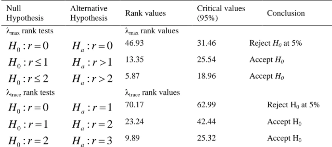
variables ensured normality of the probability distribution of the residuals in all VECM models. Both Maximum eigenvalue and Trace statistics suggest a significant long run relationship between real exports, real imports, real exchange rates and real GDP in both sub-samples.
Table 3. Cointegration test based on Johansen’s method in 1820 and 1860 Null
Hypothesis
Alternative
Hypothesis Rank values
Critical values
(95%) Conclusion
λmax rank tests λmax rank values
0
:
0r
H
H
a:
r
0
46.93 31.46 Reject H0 at 5%1
:
0r
H
H
a:
r
1
13.35 25.54 Accept H02
:
0r
H
H
a:
r
2
5.87 18.96 Accept H0λtrace rank tests λtrace rank values
0
:
0r
H
H
a:
r
1
70.17 62.99 Reject H0 at 5%1
:
0r
H
H
a:
r
2
23.24 42.44 Accept H02
:
0r
H
H
a:
r
3
9.89 25.32 Accept H0Notes: Critical values are from Osterwald-Lenum (1992). The appropriate lag lengths and the
model regarding the deterministic components in the multivariate system are set according to the AIC and SIC criteria.
Table 4. Cointegration test based on Johansen’s method in 1867 and 1910 Null
Hypothesis
Alternative
Hypothesis Rank values
Critical values
(95%) Conclusion
λmax rank tests λmax rank values
0
:
0r
H
H
a:
r
0
30.44 27.07 Reject H0 at 5%1
:
0r
H
H
a:
r
1
12.49 20.97 Accept H02
:
0r
H
H
a:
r
2
5.98 14.07 Accept H0λtrace rank tests λtrace rank values
0
:
0r
H
H
a:
r
1
51.43 47.21 Reject H0 at 5%1
:
0r
H
H
a:
r
2
20.99 29.68 Accept H02
:
0r
H
H
a:
r
3
8.49 15.41 Accept H0Notes: Critical values are from Osterwald-Lenum (1992). The appropriate lag lengths and the
model regarding the deterministic components in the multivariate system are set according to the AIC criterion.
One of the implications of the Granger representations theorem is that as long as two variables are cointegrated and each is individually integrated of order 1, then the Granger causality must exist at least in one direction. The direction of causality can be detected through the vector error correction model on which the existence of the short term causality can be detected by the joint significance of the parameters of each lagged term through the Wald-test and the long-run causality is determined by the significance of the parameter of the error correction term through the t-test.
Since the Johansen cointegration tests above suggest a unique cointegrating vector in the four-variable VAR model, Granger causality test can be performed on the coefficients of vector error correction models as depicted by the equations (3), (4), (5) and (6). Table 5 and Table 6 show results of the short run and long run Granger causality tests for the two sub-samples and Table 7 presents summaries.
In the causality tests, the emphasis is only placed on the relationship between variables of the interest in the study, namely exports, imports and GDP to test the hypotheses. Thus, presentation of the relationship between exchange rate and other variables is excluded. In the estimations, while the coefficients of error correction term with GDP and exports as dependent variables are not significant, the coefficient of error correction term with imports as dependent variable is statistically significant at the 5% significance level and its sign is negative indicating that there is a mechanism to converge short-run dynamics into long-run equilibrium.
Table 5 presents Granger causality test results for the period 1820-1860. The error correction term for cointegrating equation with GDP growth as a dependent variable is not significant at 5% level, implying that there is no long run causality running from exports and imports to GDP. In addition, the lagged coefficients of real exports are not significant at 5% level which implies that there is no evidence of causality running from exports to GDP in the short run. Similarly, the error correction term for cointegrating equation with exports as a dependent variable is not significant at 5% level, implying that there is no long run causality running from GDP and imports to exports. In addition, the lagged coefficients of GDP are not significant at 5% level which implies that there is no evidence of causality running from exports to GDP in the short run. These results indicate that the export-led growth hypothesis and growth-led exports hypothesis are not supported for the USA between 1820 and 1860. However, there is an evidence of long run causality running from exports to imports and from GDP to imports as the error correction term for cointegrating equation with imports as a dependent variable is negative and significant at 1% level in the fifth model. In addition, the Wald test in the fifth model implies the existence of one-way short run causality running from exports to imports at the
7% significance level. These outcomes indicate that growth-led imports hypothesis is supported only in the long-run. Since the Granger causality exists at least in one direction, the results in this period are in concordance with the Granger representations theorem.
In sum, Granger causality results provide evidence only for growth-led imports hypothesis in the long-run and there is no evidence of export-led growth hypothesis, growth-led exports hypothesis and import–led growth hypothesis both in the short-run and long-run for the USA between 1820 and 1860.
Impulse response functions and variance decompositions can be employed to summarize relationships among the variables in the cointegrated system. Impulse response functions show that how shocks to any one variable affect every other variable in the system and eventually feed back to the original variable itself. Variance decompositions indicate the proportion of the movements in the dependent variables that are due to their own shocks versus shocks to the other variables. Impulse responses and variance decompositions are provided for each of the four variables in the system. However, the estimations are presented only for the variable of interest, namely, GDP, exports and imports.
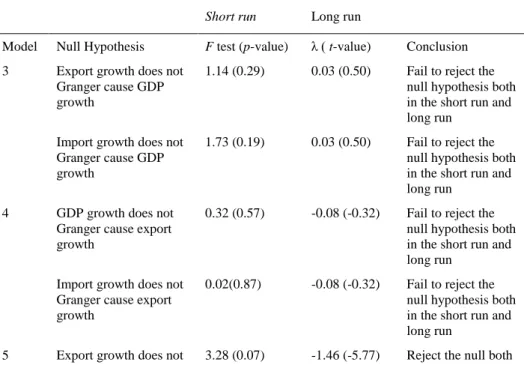
Table 5. Granger causality tests: 1820-1860
Short run Long run
Model Null Hypothesis F test (p-value) λ ( t-value) Conclusion 3 Export growth does not
Granger cause GDP growth
1.14 (0.29) 0.03 (0.50) Fail to reject the null hypothesis both in the short run and long run
Import growth does not Granger cause GDP growth
1.73 (0.19) 0.03 (0.50) Fail to reject the null hypothesis both in the short run and long run
4 GDP growth does not Granger cause export growth
0.32 (0.57) -0.08 (-0.32) Fail to reject the null hypothesis both in the short run and long run
Import growth does not Granger cause export growth
0.02(0.87) -0.08 (-0.32) Fail to reject the null hypothesis both in the short run and long run
Granger cause import growth
in the short and long run
GDP growth does not Granger cause import growth
1.01 (0.32) -1.46 (-5.77) Fail to reject the null in the short run, but reject the null in the long run
Notes: The VECMs are estimated with a constant and a lag structure determined optimally by the
AIC and SIC criteria. Diagnostic tests (not reported) conducted for various orders of serial correlation, heteroscedasticity, stability and normality. They were overall found to be satisfactory. F test is the Wald test on each lagged term. λ is an adjustment coefficient with a t test on the parameter of the error correction term.
Figure 5 shows impulse response functions and variance decompositions of each dependent variable with the ordering of the variables below. The results are consistent with the Granger causality test results. The responses of GDP and exports to the shocks are very small, except for the response of a variable to its own shock, and they die down to almost nothing after the first period. Similarly, the percentages of the GDP and export forecast variances can be attributed to shocks in GDP and export alone as opposed to other variables the throughout periods. These findings provide no supporting evidence for exports-led growth, imports-exports-led growth and growth-exports-led exports hypotheses.
In contrast to these results, the response of imports to the shocks from GDP and exports are positive and very large. The response to a shock from exports is even larger than itself in the first period. The large responses continue throughout the period. Similarly, about 20% of the import forecast variances can be attributed to shocks in GDP and exports throughout the periods. These findings provide supporting evidence for causality relationship from GDP to imports in the long run and from exports to imports in the short-run and long-short-run.
Figure 5. Impulse Response Functions and Variance Decompositions:1820-1860 -.01 .00 .01 .02 .03 .04 1 2 3 4 5 6 7 8 9 10 GDP Exports
Imports Exchange rate
Response of GDP to Cholesky One S.D. Innovations 0 20 40 60 80 100 120 1 2 3 4 5 6 7 8 9 10 GDP Exports
Imports Exchange rate
Variance Decomposition of GDP -.02 .00 .02 .04 .06 .08 .10 .12 .14 1 2 3 4 5 6 7 8 9 10 Exports GDP Imports Exchange rate
Response of Exports to Cholesky One S.D. Innovations 0 20 40 60 80 100 1 2 3 4 5 6 7 8 9 10 Exports GDP Imports Exchange rate
Variance Decomposition of Exports
-.050 -.025 .000 .025 .050 .075 .100 .125 .150 1 2 3 4 5 6 7 8 9 10 Impors GDP Exports Exchange rate
Response of Imports to Cholesky One S.D. Innovations 0 20 40 60 80 100 1 2 3 4 5 6 7 8 9 10 Imports GDP Exports Exchange rate
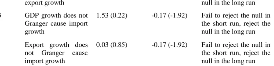
Table 6 presents Granger causality test results for the period 1867-1910. In all estimations, the coefficients of error correction term with GDP, exports and imports as dependent variables are statistically significant at 1%, 1% and 10% significance levels, respectively, and their signs are negative indicating that there is a mechanism to converge short-run dynamics into long-run equilibrium.
In contrast to the previous period, the error correction term for cointegrating equation with GDP growth as a dependent variable is significant at 1% level, implying that there is a long run causality running from exports to GDP and from imports to GDP. In addition, the lagged error terms of real exports and real imports are not significant at 5% level which imply that there is no evidence of causality running from exports to GDP and imports to GDP in the short run. These results indicate that the export-led growth hypothesis and import-led growth hypothesis are supported for the US between 1867 and 1910. There is also evidence for reverse causality relationships. The error correction term for cointegrating equation with exports as a dependent variable is significant at 1% level, implying that there is a long run causality running from GDP to exports and from imports to exports. In addition, the lagged error terms of GDP are significant at 5% level which imply that there is an evidence of causality running from exports to GDP in the short run. It can also be inferred from the estimation of the model (5) that both exports and GDP Granger cause imports in the long run as the coefficient of the error correction term is significant at 10% level. In sum, Granger causality results provide evidence for growth-led imports, import-led growth, growth-led exports and export-led growth hypotheses in the long run during the period between 1867 and 1910 in the US.
Table 6. Granger causality tests: 1867-1910
Model Null Hypothesis F test (p-value) λ ( t-value) Conclusion 3 Export growth does
not Granger cause GDP growth
0.42 (0.51) -0.03 (-4.00) Fail to reject the null in the short run, reject the null in the long run Import growth does
not Granger cause GDP growth
0.04 (0.83) -0.03 (-4.00) Fail to reject the null in the short run, reject the null in the long run 4 GDP growth does not
Granger cause export growth
4.15 (0.04) -0.22 (-2.62) Reject the null both in the short run and long run
Import growth does not Granger cause
0.14 (0.70) -0.22 (-2.62) Fail to reject the null in the short run, reject the
export growth null in the long run 5 GDP growth does not
Granger cause import growth
1.53 (0.22) -0.17 (-1.92) Fail to reject the null in the short run, reject the null in the long run Export growth does
not Granger cause import growth
0.03 (0.85) -0.17 (-1.92) Fail to reject the null in the short run, reject the null in the long run
Notes: The VECMs are estimated with a constant and a lag structure determined optimally by the
AIC and SIC criteria. Diagnostic tests (not reported) conducted for various orders of serial correlation, heteroscedasticity, stability and normality. They were overall found to be satisfactory. F test is the Wald test on each lagged term. λ is an adjustment coefficient with a t test on the parameter of the error correction term.
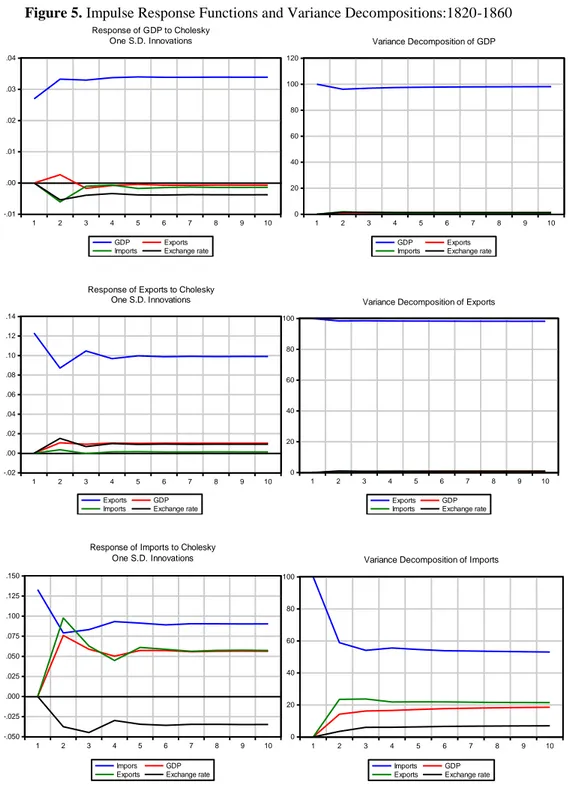
Figure 6 shows impulse response functions and variance decompositions of each dependent variable with the ordering of the variables below. The results are consistent with the Granger causality test results. The responses of imports to the shocks from GDP and exports are very large and they become larger and larger as periods have passed. Similarly, percentages of GDP forecast variances can be attributed to shocks in imports and exports are very large and they increase as periods have passed. These findings provide supporting evidence for causality relationship from exports to GDP and from imports to GDP in the long run.
The responses of exports to the shocks from GDP and imports are positive and very large. After the jump in the first period, the large responses continue throughout the period and they become larger and larger as periods have passed. Similarly, percentages of export forecast variances can be attributed to shocks in imports and exports appear very large and they gradually increase as periods have passed. These findings provide supporting evidence for causality relationship from GDP to exports and from imports to exports in the long run.
The response of imports to the shocks from GDP and exports are positive and very large. The response to a shock from exports even becomes larger than itself in the fifth period. The large responses continue throughout the period. Similarly, the percentages of the import forecast variances can be attributed to shocks in GDP and exports becomes larger and larger as periods have passed. The percentage of the import forecast variances that can be attributed to shocks in exports are larger than that of GDP throughout the period. These findings provide supporting evidence for causality relationship from GDP to imports and from exports to imports in long-run.
Figure 6. Impulse Response Functions and Variance Decompositions:1867-1910 -.03 -.02 -.01 .00 .01 .02 .03 .04 .05 1 2 3 4 5 6 7 8 9 10 GDP Exports
Imports Exchange rate
Response of GDP to Cholesky One S.D. Innovations 0 20 40 60 80 100 1 2 3 4 5 6 7 8 9 10 GDP Exports
Imports Exchange rate
Variance Decomposition of GDP -.02 .00 .02 .04 .06 .08 .10 1 2 3 4 5 6 7 8 9 10 Exports GDP Imports Exchange rate
Response of Exports to Cholesky One S.D. Innovations 0 20 40 60 80 100 1 2 3 4 5 6 7 8 9 10 Exports GDP Imports Exchange rate
Variance Decomposition of Exports
-.04 -.02 .00 .02 .04 .06 .08 .10 .12 1 2 3 4 5 6 7 8 9 10 Imports GDP Exports Exchange rate
Response of Imports to Cholesky One S.D. Innovations 0 20 40 60 80 100 1 2 3 4 5 6 7 8 9 10 Imports GDP Exports Exchange rate
Table 7 summarizes the findings from estimations for all the variables considered and for both periods.
Table 7. Summary of the Granger causality results
1820-1860 1866-1910
Direction of Causality Short-run Long-run Short-run Long-run
X→GDP - - - + GDP→X - - + + M→GDP - - - + GDP→M - + - + X→M + + - + M→X - - - +
Conclusion
In this study, the relationship between real exports, real imports and real GDP is questioned between the years 1820 and 1910 in the United States. Our aim was to determine if the nineteenth century American growth could be explained by export-led growth, growth-led exports, import-led growth and growth-led imports hypotheses. Lipsey (2000: 727) argues that through much of its history, the United States “has been pointed to as a country for which international trade was unimportant.” However the results of our study contradict with the above statement at least for the period between 1867 and 1910 and hence, attribute a larger role to international trade in American growth after the Civil War. The econometric analyses show that real exports, real imports, real exchange rate and real GDP are cointegrated for the periods 1820-1860 and 1867-1910, and therefore they are causally related. We detected a bi-directional long-run causality from exports to imports and from GDP to imports and a bi-directional short-run causality from exports to imports during the period between 1820 and 1860. However, for the period between 1867 and 1910 we detected two-way causality between all the related variables in the long run and one-way causality from GDP to exports in the short run.
Based on the estimations of and tests on the vector error correction models, we conclude that growth-led imports hypothesis is valid for both
periods. In addition, validity of growth-led export, export-led growth and import-led growth hypotheses is supported for only the 1867-1910 period. In contrast, we do not find evidence to support for export-led growth, growth-led export and import-led growth to these hypotheses in the first period. Therefore, it is safe to argue that constantly growing internal market, bringing about a constantly increasing demand, was the main determinant of growth in the pre-Civil War period. In this case, internal demand, as the main stimulant of growth, resulted in a rise in exports and imports as well, thanks to the increasing productive capacity of the nation. However, international trade became an important factor in American growth after the Civil War. These findings are in accordance with rising volume of world trade and high economic growth rates of the US economy during this period.
Reference
Abramowitz, Moses (1989), Thinking About Growth and Other Essays on Economic Growth and
Welfare (New York: Cambridge University Press).
Acemoglu, Daron (2009), Introduction to Modern Economic Growth (Princeton, NJ: Princeton University Press).
Acemoglu, Daron and James A. Robinson (2012), Why Nations Fail: The Origins of Power,
Prosperity and Poverty (London: Profile Books).
Asteriou, Dimitrious and Stephen G. Hall (2011), Applied Econometrics (New York, NY, USA: Palgrave Macmillan).
Atack, Jeremy and Peter Passell (1994), A New Economic View of American History from Colonial
Times to 1940 (New York: W.W. Norton & Company, Inc).
Atack, Jeremy, Fred Bateman, F. and Robert A. Margo (2008), “Steam Power, Establishment Size, and Labor Productivity Growth in Nineteenth Century American Manufacturing”,
Explorations in Economic History, 45: 185-198.
Awokuse, Titus O. (2006), “Export-Led Growth and the Japanese Economy: Evidence from VAR and Directed Acyclic Graphs”, Applied Economics, 38 (5): 593-602.
Bensel, Richard F. (2000), The Political Economy of American Industrialization, 1877-1900 (New York: Cambridge University Press).
Braudel, Fernand (1995), A History of Civilizations (New York: Penguin).
Broadberry, Stephen N. and Douglas A. Irwin (2006), “Labor Productivity in the United States and the United Kingdom During the Nineteenth Century”, Explorations in Economic History, 43: 257-279.
Chang, Ha-Joon (2002), Kicking Away the Ladder: Development Strategy in Historical Perspective (London: Anthem Press).
Davis, Lance E., Richard A. Easterlin and William N. Parker. eds. (1972), American Economic
Growth: An Economist’s History of the United States (New York: Harper & Row).
Dickey, David A. and Wayne A. Fuller (1979), “Distribution of the Estimators for Autoregressive Time Series with a Unit Root”, Journal of the American Statistical Association, 74 (366): 427-431.
Dufoura, Jean-Marie, Denis Pelletierb, Eric Renault (2006), "Short run and long run causality in time series: inference”, Journal of Econometrics, 132: 337–362.
Elliott, Graham, Thomas J. Rothenberg and James H. Stock (1996), “Efficient Tests for an Autoregressive Unit Root”, Econometrica, 64 (4): 813-836.
Engle, Robert. F. and Clive W. J. Granger (1987), “Co-integration and Error Correction: Representation, Estimation and Testing”, Econometrica, 55 (2): 251-276.
Fite, Gilbert C. and Jim E. Reese (1973), An Economic History of the United States (Boston: Houghton Mifflin Company).
Gallman, Robert E. (2000), “Economic Growth and Structural Change in the Long Nineteenth Century,” in Engerman, Stanley L. and Robert E. Gallman eds., The Cambridge
Economic History of the United States Vol. II, The Long Nineteenth Century (Cambridge:
Cambridge University Press): 1-55.
Harris, Richard and Robert Sollis (2003), Applied Time Series Modelling and Forecasting (West Sussex: John Wiley & Sons Ltd).
Johansen, Soren (1988), “Statistical Analysis of Cointegration Vectors”, Journal of Economics
Dynamics and Control, 12: 231-54.
Johnston, Louis and S. H. Williamson (2017), “What Was the U.S. GDP Then?” MeasuringWorth, https://www.measuringworth.com/usgdp.
Kennedy, Peter (2003), A Guide to Econometrics (Cambridge, MA: The MIT Press).
Kravis, Irving B. (1972), “The Role of Exports in Nineteenth-Century United States Growth”,
Economic Development and Cultural Change, 20 (3): 387-405.
Kwiatkowski, Denis, Peter C. B. Phillips, Peter Schmidt and Yongcheol Shin (1992), “Testing the Null Hypothesis of Stationarity against the Alternative of a Unit Root”, Journal of
Econometrics, 54: 159-178.
Landes, David S. (1999), The Wealth and Poverty of Nations (New York: W.W. Norton & Company).
Lipsey, Robert E. (2000), “U.S. Foreign Trade and the Balance of Payments, 1800-1913,” Engerman, Stanley L. and Robert E. Gallman (Eds.), The Cambridge Economic History of
the United States Vol. II, the Long Nineteenth Century (Cambridge: Cambridge University
Press), 685-732.
Maddala, Gangadharrao S. and In-Moo Kim (1998), Unit Roots, Cointegration and Structural
Change (Cambridge: Cambridge University Press).
Marin, Dalia (1992), “Is the Export-Led Growth Hypothesis Valid for Industrialized Countries?”, The
Review of Economics and Statistics, 74 (4): 678-688.
North, Douglass C. (1961), The Economic Growth of the United States, 1790-1860 (Englewood Cliffs, NJ: Prentice-Hall, Inc).
O’Sullivan, John and Edward F. Keuchel (1989), American Economic History: From Abundance to
Osterwald-Lenum, Michael (1992), “A Note with Quantiles of the Asymptotic Distribution of the Maximum Likelihood Cointegration Rank Test Statistic”, Oxford Bulletin of Economics and
Statistics, 54: 461-472.
Perron, Pierre (1989), “The Great Crash, the Oil Price Shock and the Unit Root Hypothesis”,
Econometrica, 57 (6): 1361-1401.
Phillips, Peter C. B. and Sam Ouliaris (1990), “Asymptotic Properties of Residual Based Tests for Cointegration”, Econometrica, 58 (1): 165-93.
Phillips, Peter C. B. and Pierre Perron (1988), “Testing For a Unit Root in Time Series Regression”,
Biometrika, 75: 335-346.
Ratner, Sidney, James H. Soltow and Richard Sylla (1979), The Evolution of the American
Economy: Growth, Welfare and Decision Making (New York: Basic Books, Inc.
Publishers).
Rousseau, Peter L. and Richard Sylla (2005), “Emerging Financial Markets and Early US Growth”,
Explorations in Economic History, 42: 1-26.
Tuttle, Frank W. and Joseph M. Perry (1970), An Economic History of the United States (Cincinnati: South-Western Publishing Company).
Vergil, Hasan and M. Erdem Özgür (2013), “American Growth and Napoleonic Wars”,
Panoeconomicus, 60 (5): 649-666.
Zivot, Eric and Donald Andrews (1992), “Further Evidence of Great Crash, the Oil Price Shock and Unit Root Hypothesis”, Journal of Business and Economic Statistics, 10 (3): 251-270.