Turkish credit default swap and relationship with financial indicators

(1)

i

TURKISH CREDIT DEFAULT SWAP

AND

RELATIONSHIP WITH FINANCIAL INDICATORS

DİLEK ÖZKAPLAN

108673014

İSTANBUL BİLGİ ÜNİVERSİTESİ

SOSYAL BİLİMLER ENSTİTÜSÜ

BANKACILIK FİNANS YÜKSEK LİSANS PROGRAMI

ÖĞR.GÖR. ALİ BATU KARAALİ

2011

(2)

ii

Turkish Credit Default Swaps and Relationship with Financial

Indicators

Türkiye Kredi Temerrüt Takasları ve Finansal Göstergelerle

İlişkisi

Dilek Özkaplan

108673014

Öğr. Gör. Ali Batu Karaali

: ...

Yrd. Doç. Dr. Cenktan Özyıldırım

: ...

Öğr. Gör. Kenan Tata

: ...

Tezin Onaylandığı Tarih

: ...

Toplam Sayfa Sayısı

: 52

Anahtar Kelimeler (Türkçe) Anahtar Kelimeler (İng.)

1) Kredi Temerrüt Takası 1) Credit Default Swap

2) Birim Kök 2) Unit Root

3) Granger Nedensellik Testi 3) Granger Causality Test

4) Regresyon Analizi 4) Regression Analysis

(3)

iii

I hereby declare that all information in this document has been obtained and presented in accordance with academic rules and ethical conduct. I also declare that, as required by these rules and conduct, I have fully cited and referenced all material and results that are not original to this work.

Name, Last name: Dilek ÖZKAPLAN Signature:

(4)

iv

Abstract

The credit default swap (CDS) is the building stone of hedging strategies for credit exposures, and basis of more advanced credit derivative products. The CDS market has appeared to become a major asset class in the capital markets. One largely confined to banks, to market participants have expanded to include insurance companies, hedge funds, mutual funds, pension funds, and other investors looking for yield enhancement or credit risk transference. The literature review presents the recent work on interactions of credit default swap and other variables.

The scope of this study is to find out if there is a relationship separately between CDS spreads and financial indicators as Eurobond, Dow Jones Index, Istanbul Stock Exchange Index (ISE–100), Foreign exchange currency (Fx) rates. In our empirical work, we collect CDS, Eurobond and Dow Jones data from Bloomberg data provider, ISE–100 closing price data from ISE web site and Fx –TRY currency rates from web site of Central Bank of the Republic of Turkey for dates from March 3rd, 2002 to January 22nd, 2010. E-views 5 program is used for One Variable and Multivariable Regression, Correlation, Granger Causality Tests and Vector Autoregression Tests . Dow Jones rates, and the way of the interaction runs from Eurobond and Dow Jones to CDS. Results enable to interpret the relationship between CDS–ISE 100 and CDS–currency rates. Causality runs for both variables from CDS.

(5)

v To life,

(6)

vi

Acknowledgements

First of all, I would like to express my gratitude to my dissertation advisor Ali Batu Karaali (Assistant General Manager-Treasurer of HSBC Bank). I appreciate his intellectual comments, knowledge and assistance which helped me a lot in preparing my thesis. With his instructions I have started to be interested in derivative markets and especially credit default swaps. I am also thankful to Ferhat Kasap for his help while preparing my thesis. I would also like to thank my colleagues from Turkland Bank and HSBC Bank for their understanding in this period. Special thanks to Assistant General Manager (Treasurer of Turkland Bank) Münevver Eröz for her comments, thanks to Sevgi Üstün and Didem Çalışkan for their support. Very special thanks go to PhD Candidate in Economics Coşkun Tarkoçin from HSBC, who became more of a mentor and a friend than a partner, and who taught almost everything I have learned in my work life and encouraged me to start a graduate program.

Finally and most importantly, I would like to thank my family who has never stopped supporting and encouraging me through my entire life. Without their love and belief I would do nothing.

(7)

vii

List of Tables

Table Page

1 Credit Product Composition Percent…...8

2 Buyers of Protection Percent…...9

3 Sellers of Protection Percent…...9

4 Descriptive Statistics of Data…...13

5 Descriptive Statistics of Turkey CDS_5Y by Years…...13

6 Descriptive Statistics of Turkey Eurobond by Years…...14

7 Descriptive Statistics of ISE 100 By Years………...16

8 Descriptive Statistics of Dow Jones by Years…………...17

9 Descriptive Statistics of Fx Basket by Years…………...18

10 Correlations among Variables………...19

11 ADF Unit Root Test on Turkey_CDS5Y...21

12 ADF Unit Root Test on Eurobond...21

13 ADF Fuller Unit Root Test on ISE_100...22

14 ADF Unit Root Test on Dow Jones...22

15 ADF Unit Root Test on Fx Basket...23

16 ADF Unit Root Test on Turkey_CDS5Y…...23

17 ADF Unit Root Test on Eurobond...23

18 ADF Unit Root Test on ISE_100...24 19 ADF Unit Root Test on Dow Jones...24

20 ADF Unit Root Test on Fx Basket...24

21 Descriptive Statistics of Growth Ratios of Variables...25

22 Correlations among Growth Ratios of Variables...25

23 Regression Output Table Turkey CDS 5Y-ISE100...31

24 Regression Output Table Turkey CDS 5Y-Dow Jones...32

25 Regression Output Table Turkey CDS 5Y-Fx Basket...34

26 Regression Output Table Turkey CDS 5Y-Eurobond...35

27 Multivariate Regression Output Table...36

28 Wald Test...38

29 Determining Compatible Number of Lags...40

30 Pairwise Granger Causality Tests...41

(9)

ix

List of Figures

Figure Page

1 Growth of Credit Default Swaps...7

2 Total Derivatives and Credit Default Swaps...8

3 CDS5Y Spreads in Basis Points...14

4 Eurobond Yields in Percentage...15

5 ISE 100 Closing Prices...16

6 Dow Jones...17

7 Fx Basket Rates...18

8 Graphs For Non-Stationary and Stationary Time Series...25

9 CDS-ISE 100 Scatter...32

10 CDS-Dow Jones Scatter...33

11 CDS-Fx Basket Scatter...34

12 CDS-Eurobond Scatter...36

13 CDS Against All Scatter...37

(10)

x

Abbreviations

ADF Augmented Dickey-Fuller Test

AIC Akaike Information Criterion

AIG American International Group Insurance Company

BBA British Bankers Association

BISTRO Broad Index Secured Trust Offering

CBRT Central Bank of the Republic of Turkey

CDS Credit Default Swap

DW Durbin-Watson

DCDS First Difference of CDS data

DDow Jones First Difference of Dow Jones data

DEurobond First Difference of Eurobond data

DFx basket First Difference of Foreing Exchange Currency data

DISE First Difference of Istanbul Stock Exchange data

ESS Explained Sum of Squares

FAS Financial Accounting Standarts

FPE Final Prediction Error

Fx Foreign Exchange

HQ Hannan-Quinn Information Criterion

ISDA International Swaps and Derivatives Association

ISE Istanbul stock Exchange

iBoxx Bond Market Indices

iTraxx A group of international credit derivative indexes that

are monitored by the International Index Company (IIC)

OLS Ordinary Least Squares

OTC Over the Counter

RSS Residual Sum of squares

SC Schwarz Information Criterion

SD Standard Deviation

SE Sum of Errors

Trac-x Transport Capacity Exchange

TSS Total Sum of Squares

(11)

1

1. INTRODUCTION

Credit Default Swap (CDS) has been one of the most fascinating developments of last two decades in financial markets, particularly in credit markets. CDS market is used to differentiate credit risk from other risks. In addition, it provides an efficient way to trade credit risk. The big volume of CDS trading, flourishing of CDS related products and its phenomenal role in current credit crisis indicate the importance of this relatively new financial product.

The purpose of this study is to explore the interactions and causality relationship between CDS and other financial indicators. This paper is organized as follows: In section 1, a summary of CDS market is given. In section 2, general information about previous research and an analysis on related data is provided. Finally, in last section our results have been summarized.

1.1 CREDIT DEFAULT SWAPS: THE BASICS

Credit derivatives are exciting innovations in financial markets. They give the potential to companies to trade and manage credit risk. The most popular credit derivative is a credit default swap (CDS) (Hull & White, 2000). A CDS is a contract that provides insurance against the risk of default by a particular company or even a particular debt. The contract will determine the reference entity or the reference liability. The reference entity means the issuer of the debt instrument. It could be a corporation, a sovereign government bond, or a bank loan (Fabozzi, 2004).

Credit event means a default by the company. The buyer of the CDS accepts to make periodic payments to the seller and these payments end if there is a default by the reference entity or a default by the counterparty (Hull, 2001).

(12)

2

Whenever a credit event exists, usually it requires a final accrual payment by the buyer. The total par value of the reference entity that can be sold is known as the swap's notional principal. The buyer of CDS has the right to sell a particular entity, issued by the company, for its par value when a credit event occurs (Hull, 2004).

The swap then could be settled by either a physical delivery or a cash delivery. If the contract of the swap requires physical delivery, the swap buyer delivers the reference entity to the seller in exchange for their par value. When the contract requires cash delivery, the calculation agent asks the dealers to determine the current market price, P, of the reference entity after some specified number of days of the credit event. The cash delivery is then a settled (100-P) percent of the notional principal (Hull & White, 2000).

In a credit default swap, the protection buyer makes a payment (a fee), called swap premium, to the protection seller. In the end there exists the right to receive a payment depends on the default of the reference entity. The payments made by the protection buyer are called the premium leg; the contingent payment that might have to be made by the protection seller is called the protection leg (Fabozzi, 2001).

These contracts are logically default options, not swaps. The difference from a regular option is that the cost of the option, which is called the premium, is paid in a deferred payment instead of in an advance payment. When the premium is paid in advance, these contracts might be called default put options. Default swaps and default options are not the same instruments, however, because a default swap requires deferred payments only until a triggering default event exists (Jorion, 2003).

This financial derivative has been driven by the demand from banks and insurance companies to protect their underlying entities against credit

(13)

3

defaults. Hedge funds and investment banks' also need their private trading desks for more liquid instruments to speculate on credit risk. Trading in CDS contracts can have a wide impact on market because of its fantastic growth. Because of the rapid growth of market, a number of policy concerns about market stability and risk of adverse selection have been raised by the regulatory supervision of the CDS market. This would affect both the tendency of investors to trade in the market and therefore the liquidity of CDS contracts (Tang & Yan, 2007).

There are different kinds of credit default swaps: Binary credit default swaps, basket credit default swaps, contingent credit default swaps, and dynamic credit default swaps. In a binary credit default swap, the payment when the default exists, is a specific dollar amount. In a basket credit default swap, there is a specified group of reference entities and payment is done when one of these reference entities defaults. In a contingent credit default swap, the payment requires a credit event together with an additional trigger. This trigger might be a credit event related to another reference entity or a specified movement in some market variable. In a dynamic credit default swap, the notional amount determining the payoff is linked to the mark-to-market value of a portfolio of swaps (Hull & White, 2000).

Credit default swaps can be used by financial investors in different ways such as hedging and speculating. Example of the former one is that; investing in a risky bond is equal to investing in a risk-free bond and selling a credit default swap together. The risky bond price is a and promises to pay a+2x in maturity. The risk-free price is a+x. Buying the risky bond is then equal to buying the risk-free bond at a+x and selling a credit default swap worth x at the same time. The first cost is the same in two conditions, a. If the company defaults, the final payment will be the same. The protection buyer reduces exposure to the reference entity but accepts new credit exposure to the seller. To be effective, there has to be a low correlation

(14)

4

between the default risk of the underlying credit and of the counterparty (Jorion, 2003). Example of the latter way of using CDS is that; investors can go both long and short positions in a particular credit without holding the underlying entity. This makes a credit default swap more accessible and easier to trade than its underlying reference entity. There are tradable CDS indexes (iBoxx, Trac-x, LevX, LCDX) which allow financial investors quick and easy ways to buy and sell credit risk (Byström, 2005). In June 21, 2004, the two main CDS indexes, iBoxx and Trac-x, were merged to form the CDX in North America, emerging markets and the iTraxx in Europe and Asia. Markit became the administrator for the CDX and calculation agent for iTraxx and acquired both families of indices in November 2007, and owns the iTraxx, CDX, LevX, and LCDX indices for derivatives, and the iBoxx indices for cash bonds (Markit, 2008).

1.2 HISTORY OF CREDIT DEFAULT SWAPS

During the recent credit crisis, Credit Default Swaps has received great attention because of toxic assets’ huge demand on financial markets. In 1997, a credit derivative team at JP Morgan’s (New York City, USA) launched CDSs with newspaper articles. At that time, they named this new derivative type as BISTRO (not CDS) which stands for Broad Index Secured Trust Offering. This product was a later stage in the development of CDS trading and the credit derivative market (Levy, 2009).

David Mengel (2007) describes evolution of CDS market from 1980 until today in four stages in his overview of credit derivative market.

The first stage of the credit derivative trading can be characterized as a defensive step. It mainly includes attempts taken by major banks to eliminate some of the credit exposure on their balance sheets. According to regulation (FAS 133)1, reporting standards for derivative instruments are

1

(15)

5

considered as a hedge of the exposure to the fair value of a liability, a firm commitment or a cash flow. This regulation enables a firm to reduce its credit exposure from its balance sheet. This stage took place in the late 1980s and early 1990s. During this period, banks had sold their loans to the other banks or private investors in return for periodic payments by using product similar to CDSs. When default happened, similar to the CDS contract, the loans or bonds that have credit exposure were being delivered to the investor, who would take the losses instead of the bank.

The second stage took place between 1991 and the late 1990s. The main change during this stage is the development of financial engineering technology for pricing the transfer of credit risk. The BISTRO was a financial tool designed to remove loans from banks’ balance sheets and in turn free up cash. This product has worked by establishing a new company by the bank. The new company has bought the debt of the banks’ balance sheets, and then issued bonds that were sold to different investors. Any investor who bought these bonds was betting against the default of the original borrowers, to whom the bank established in the first place.

The third stage is the mature CDS market which exist today and the standardization of its trade and contractual terms. During this stage, single name CDS contracts were developed and started being traded over-the-counter (OTC). Moreover, some new regulations were developed to organize and guide trade and define capital requirements. The International Swaps and Derivatives Association (ISDA) introduced the standardized contractual agreement, which offers the standard CDS agreement accepted by most of the traders today. Counterparty risk management begins with ISDA or other related transaction documentation. This is followed by measurement of both current exposure and potential losses if default were to occur in the future and finally collateral net exposures are made (Chaplin, 2005).

(16)

6

The fourth stage is the expansion of the types of players engaged in trading in the CDS market. Originally CDS trading was centered around banks’ activities, this stage saw the entry of hedge funds as major players into CDS market. Hedge funds started to take the position of sellers or buyers, based on seeking exposure or hedging the credit risk. The entry of the hedge funds into the CDS market also introduces new trading motivations. Hedge funds are now using CDSs to trade misprices in credit risk, to remove unwanted credit risk from their portfolio and to trade CDS bond basis spreads. This fast dynamic hedge fund activity in the CDS market has contributed to increased trade volume and increased liquidity which has resulted in better price discovery (Mengle, 2007).

1.3 MARKET DATA

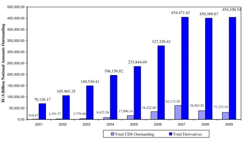
Since the credit derivates are mostly traded OTC, it is hard to generate an exact estimate of its gross market size. However, it is clear that the CDS market has the largest share in the credit derivative market, and the total credit derivative market has experienced a dramatic growth over the past decade. According to ISDA market survey, estimated gross market has reached to 62 trillion dollars in 2007 and it came down to 31 trillion dollars at the end of the second quarter of 2009. Figure 1 provides estimates for single name CDSs from 2001 to 2009, and Figure 2 provides estimates of the credit derivatives market in general (includes; interest rate swaps, currency swaps, credit default swaps and equity swaps) compared to CDS. As it can be seen in Figure 2, the credit derivative market had almost doubled from 2006 to 2007. The CDS market grew more than 25 trillion dollars during the same period. In 2003, the total CDS global notional amount was 3.7 trillion dollars, indicating a market growth of approximately 1,000 percent by 2007.

(17)

7

Source: ISDA Market Surveys,2001-1H2009 631.50 1,563.48 34,422.80 2,687.91 5,441.86 31,223.10 54,611.82 45,464.50 26,005.72 12,429.88 3,779.40 2,191.57 918.87 8,422.26 38,563.82 62,173.20 17,096.14 0.00 10,000.00 20,000.00 30,000.00 40,000.00 50,000.00 60,000.00 70,000.00 2001 2002 2003 2004 2005 2006 2007 2008 2009 $ U .S .B il li o n N o ti o n a l A m o u n ts O u ts ta n d in g 1H 2H

Figure 1. Growth of Credit Default Swaps

Source: ISDA Market Surveys,2001-1H2009 70,126.17 105,965.35 149,530.41 196,156.82 235,844.69 327,329.42 450,369.67 918.87 2,191.57 3,779.40 8,422.26 17,096.14 34,422.80 62,173.20 38,563.82 31,223.10 454,100.54 454,471.62 0.00 50,000.00 100,000.00 150,000.00 200,000.00 250,000.00 300,000.00 350,000.00 400,000.00 450,000.00 500,000.00 2001 2002 2003 2004 2005 2006 2007 2008 2009 $ U .S .B il li o n N o ti o n a l A m o u n ts O u ts ta n d in g

Total CDS Outstanding Total Derivatives

Figure 2. Total Derivatives and Credit Default Swaps

Average notional amounts for individual deals vary by region and sector. In North America, average notional amounts for investment grade CDSs are between 10 and 20 million dollars. Concerning CDSs with reference entities below investment grade, the numbers are about half of the size. In Europe, average notional amounts for investment grade CDSs are around 10 million

(18)

8

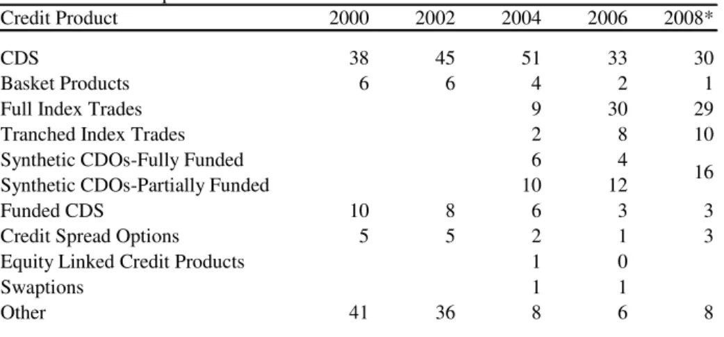
euro. The 5-year maturity is traditionally the most liquid contract, but liquidity increases for longer maturities up to 10 year ones (Mengle, 2007). Table 1 presents a market breakdown with respect to product type between 2000 and 2008. As it can be seen, the market share of single name CDS had increased from 2000 until 2004. During this period it has increased from 30 percent to above 50 percent, and then it started to decrease back to 33 percent. After their emergence, CDS indices has quickly become rival to single name CDSs. Their market share has changed from 9 percent in 2004 to 30 percent in 2006. Single CDSs and CDS indices comprise over 60 percent of the credit derivative market share together. CDS derivative, such as options, still do not comprise a large share of the market (1-5 percent between 2000-2008).

Table 1 Credit Product Composition Percent Credit Product Composition Percent

Credit Product 2000 2002 2004 2006 2008*

CDS 38 45 51 33 30

Basket Products 6 6 4 2 1

Full Index Trades 9 30 29

Tranched Index Trades 2 8 10

Synthetic CDOs-Fully Funded 6 4

Synthetic CDOs-Partially Funded 10 12

Funded CDS 10 8 6 3 3

Credit Spread Options 5 5 2 1 3

Equity Linked Credit Products 1 0

Swaptions 1 1

Other 41 36 8 6 8

*Forecast

Source: Brititish Bankers Association(2006), Mengle (2007), Bank of America (2008)

16

The market breakdown for sellers and buyers is shown in Table 2 and 3. The data indicates couple interesting patterns. First, while banks are still the main players in the market both as the seller and buyer, their market share

(19)

9

had decreased at the expense of hedge fund activity. In 2000, the banks’ share among CDS buyers was 81 percent, and 63 percent among CDS sellers, respectively. On the other hand, Hedge Funds had 3 and 5 percent in corresponding sides in that year. In 2006, banks’ activity as buyer dropped to 59 percent, and to 44 as the seller, respectively. In contrast, in this year hedge funds had increased their market shares dramatically both as seller and buyer to 28 percent as buyer and to 32 percent as seller.

Table 2 Buyers of Protection Percent

Credit Product 2000 2002 2004 2006 Banks 81 73 67 59 Banks-Trading Activities 39 Banks-Loan Portfolio 20 Insurers 7 6 7 6 Hedge Funds 3 12 16 28

Pension & Mutual Funds 2 3 6 4

Corporates 6 4 3 2

Other 1 2 1 1

Source: Brititish Bankers Association(2006), Mengle (2007)

Table 3 Sellers of Protection Percent

Credit Product 2000 2002 2004 2006 Banks 63 55 54 44 Banks-Trading Activities 35 Banks-Loan Portfolio 9 Insurers 23 33 20 17 Hedge Funds 5 5 15 32

Pension & Mutual Funds 5 5 8 7

Corporates 3 2 2 1

Other 1 0 1 1

(20)

10

Another interesting point is the net exposure of each sector to credit risk. While hedge funds are fairly balanced between their long and short position in credit risk, banks are net buyers of protection, and insurance companies are net sellers of protection. Moreover, when we look at the different applications of CDS activity within the banks’ sector, their activity is fairly balanced in exposure to credit risk, similarly for hedge funds. The source of net protection buying CDSs in banks results from their loan portfolio activity. This naturally requires more hedging of credit risk rather than exposure to it. Insurance companies, on the other hand, are net sellers of credit protection, traditionally having a share of between 20 to 30 percent as the seller, compared to a share of 6 to 7 percent as the buyer. Indeed, this fact is consistent with their function as insurance providers. In this way they gain exposure to risk. Also, it sheds light on the recent credit crisis and the collapse of the mega insurance company AIG. AIG has suffered from CDS activity and eventually brought the company bankruptcy.

(21)

11

2. EMPIRICAL ANALYSIS

2.1 LITERATURE REVIEW

The market for Credit Default Swaps (CDSs) has been growing very quickly in the last twenty years and during the credit crisis, the role of the CDS market has been drawing greater attention. Focusing on the market for CDS contracts, there exist many studies about the relationship among CDS prices and financial indicators.

Houweling and Vorst (2002) and Hull (2003) both argue that when the USD swap rate is used as risk-free rates, the price discrepancies between bond spread and CDS rates are quite small both in the short run and the long run. Longstaff (2003) who finds that both CDS and stock markets lead the bond market, but no clear lead-lag relationship was identified between CDS markets and stock markets. However, Chan-Lau and Kim (2004) find no equilibrium price relationship between sovereign CDS and sovereign bond markets, although prices converge in the long term. Haibin (2004) finds the price discrepancy between CDS rates and yield spreads very substantial in the short run. Blanco (2004) analysis dynamic relationship between investment-grade bonds and credit default swaps, and conclude that CDS rates is the upper bound and yield spread is the lower bound of the credit risk premium. Neftci, Santos and Lu (2004) find the information that helps to predict defaults and the succeeding financial crises with the difference between the CDS rate and the bond risk premium. Bystrom (2005) compares CDS spreads and stock prices using the European iTraxx CDS indices and finds that stock prices slightly lead the CDS market. He also finds a positive correlation between CDS prices and stock volatilities; CDS spreads tend to increase with increasing CDS stock price volatilities. Alexandar and Kaeck (2008) find that lead-lag relationship between stocks

(22)

12

and CDS is a regime dependent one. They show how the CDS market is extremely sensitive to stock volatilities during period of CDS market turbulence, whereas under ordinary market circumstances CDS spreads are sensitive to stock returns than they are to stock volatilities.

In the context of the above literature, this study addresses the relation among credit risk as expressed CDS spreads and other financial indicators such as Fx basket, Dow Jones Index, Eurobond rates and stock exchange returns.

2.2 DATA AND DESCRIPTIVE STATISTICS

Raw data of this study covers the time period of 8 years between March 3rd

2002 and January 22nd 2010, 1896 daily data and holidays were excluded. The complete data set is used for extracting the general pattern and behavior of Turkish CDS throughout various financial indicators and also for descriptive statistics. CDS, Eurobond and Dow Jones Index are provided from Bloomberg. Stock Price Index is provided from Istanbul Stock Exchange 100 closing price. Fx (TRY against Euro and Dollar) rates are provided from Central Bank of the Republic of Turkey (CBRT)’s web site and calculated Fx basket with fifty percent of both rates. From the beginning of 2005, CBRT removed 6 zeros form currency and made the equation of 1 New Turkish Lira to 1,000,000 Old Turkish Liras. Therefore, data before 2005 were divided to 1,000,000 to have the appropriate data set.

The mean CDS5Y spread for the data set is 393.93 basis points with standard deviation of 285.07. The difference between minimum and maximum values of variables is quite high and that cannot be undervalued. The mean of Eurobond yields is 8.53 with 1.92 standard deviation. Maximum value of 1896 observations is 14.55, which shows there have been some picks during sample years. The mean of ISE 100 prices is 30,158.78 with standard deviation of 13,912.95. Maximum value is 58,522.07 which is four times bigger than its standard deviation. The mean

(23)

13

of Dow Jones is 10,492.47 and mean of Fx basket is 1.60, standard deviation of former is 1,611.84 and latter is 0.14 (see Table 4).

Table 4 Descriptive Statistics of Data Set Proper

Name

Number of

Observations Mean

Standard

Deviation Maximum Minimum

CDS5Y 1896 393.93 285.07 1,416.88 116.55

Eurobond 1896 8.53 1.92 14.55 6.16

ISE100 1896 30,158.78 13,912.95 58,522.07 8,730.91

Dow Jones 1896 10,492.47 1,611.84 14,164.53 6,547.05

Fx Basket 1896 1.60 0.14 2.03 1.21

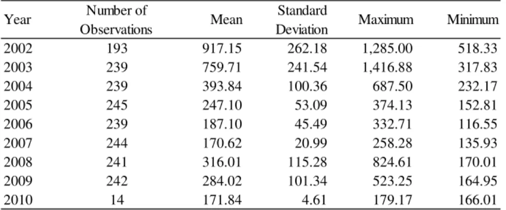
The data set become increasingly robust over time with the number of 193 observations per year in 2002, 239 in 2003, 2004 and 2006, 245 in 2005, 244 in 2007, 241 in 2008, 242 in 2009 and 14 observations per year in 2010 (see Table 5 and Figure 3). Default swap spreads vary over time with spreads historically high levels in 2002 and reverting back to an average of 170.62 basis points in 2007.

Table 5 Descriptive Statistics of Turkey CDS_5Y by years

Year Number of

Observations Mean

Standard

2002 193 917.15 262.18 1,285.00 518.33 2003 239 759.71 241.54 1,416.88 317.83 2004 239 393.84 100.36 687.50 232.17 2005 245 247.10 53.09 374.13 152.81 2006 239 187.10 45.49 332.71 116.55 2007 244 170.62 20.99 258.28 135.93 2008 241 316.01 115.28 824.61 170.01 2009 242 284.02 101.34 523.25 164.95 2010 14 171.84 4.61 179.17 166.01

(24)

14 0 200 400 600 800 1000 1200 1400 1600 2002 2003 2004 2005 2006 2007 2008 2009 TURKEY - CDS5Y

Figure 3 CDS5Y spreads in basis points

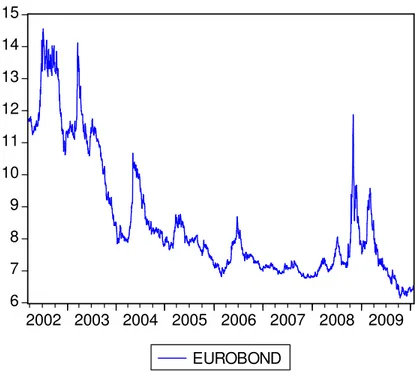
Table 6 reports the statistics for the common factors which include Eurobond yields in percentage. As shown in the table, the spot yields are decreasing with a positive mean. Historically high levels were shown in 2002 with 14.55 in percentage and decreasing level until 6.53 by the year 2010. During 2008 there is a more volatile view because of the effects of the global crisis (See Figure 4).

Table 6 Descriptive Statistics of Turkey Eurobond by years

Year Number of

Observations Mean

Standard

2002 193 12.48 1.07 14.55 10.63 2003 239 10.83 1.18 14.11 8.42 2004 239 8.62 0.75 10.67 7.77 2005 245 7.94 0.35 8.76 7.15 2006 239 7.42 0.39 8.68 6.82 2007 244 7.02 0.14 7.31 6.77 2008 241 7.64 0.89 11.87 6.79 2009 242 7.23 0.85 9.58 6.16 2010 14 6.41 0.04 6.53 6.35

(25)

15 6 7 8 9 10 11 12 13 14 15 2002 2003 2004 2005 2006 2007 2008 2009 EUROBOND

Figure 4 Eurobond yields in percentage

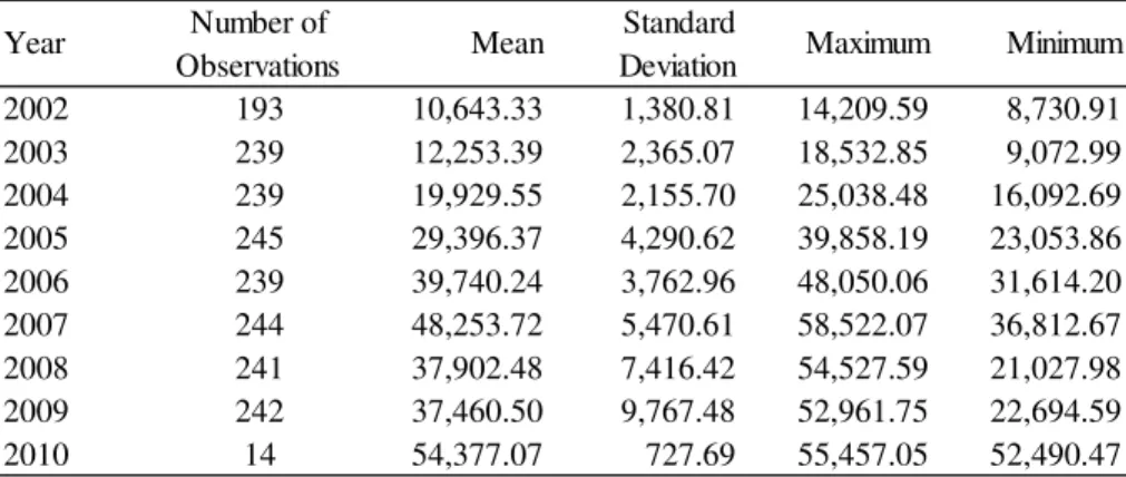
The mean ISE prices for the data set are 10,643.33 in 2002 and increasing to 37,460.50 in 2009 with standard deviation of 9,767.48. The mean is 54,337.07 for the first fourteen days of 2010. When we look at the minimum prices of the years after 2004, we could see that they have higher than the years before 2004. We can rush to the conclusion of different trends of these years (see Table 7). As we could see in the graph of ISE (Figure 5), it has an increasing trend until 2008. It again refers to global crisis and makes a downtrend. During the recovery period it rises sharply and returned to its level before crisis. As we mentioned before, the minimum price level is not as low as beginning years.

Table 8 reports the statistics for Dow Jones prices. As shown in table, means are increasing until the end of 2007 with the standard deviation of 525.48 and starts decreasing very sharply. Historically the highest price is in 2007

(26)

16 Table 7 Descriptive Statistics of ISE 100 by years

Year Number of

Observations Mean

Standard

2002 193 10,643.33 1,380.81 14,209.59 8,730.91 2003 239 12,253.39 2,365.07 18,532.85 9,072.99 2004 239 19,929.55 2,155.70 25,038.48 16,092.69 2005 245 29,396.37 4,290.62 39,858.19 23,053.86 2006 239 39,740.24 3,762.96 48,050.06 31,614.20 2007 244 48,253.72 5,470.61 58,522.07 36,812.67 2008 241 37,902.48 7,416.42 54,527.59 21,027.98 2009 242 37,460.50 9,767.48 52,961.75 22,694.59 2010 14 54,377.07 727.69 55,457.05 _52,490.47 0 10000 20000 30000 40000 50000 60000 2002 2003 2004 2005 2006 2007 2008 2009 ISE - 100

Figure 5 ISE 100 closing prices

with 14,164.53 and the lowest price is in 2009 with 6,547.05. The 2002 index has an increasing trend until 2008, like other indicators we are studying. The Dow Jones trend and falling down could be seen in Figure 6.

(27)

17 Table 8 Descriptive Statistics of Dow Jones by years

Year Number of

Observations Mean

Standard

2002 193 8,983.30 828.58 10,479.84 7,286.27 2003 239 9,016.76 695.96 10,453.92 7,524.06 2004 239 10,310.31 244.36 10,854.54 9,749.99 2005 245 10,548.94 199.30 10,940.55 10,012.36 2006 239 11,412.31 495.71 12,510.57 10,667.39 2007 244 13,173.98 525.48 14,164.53 12,050.41 2008 241 11,293.76 1,521.26 13,058.20 7,552.29 2009 242 8,860.95 1,011.45 10,548.51 6,547.05 2010 14 10,581.31 142.27 10,725.43 10,172.98 6000 7000 8000 9000 10000 11000 12000 13000 14000 15000 2002 2003 2004 2005 2006 2007 2008 2009 DOW JONES

Figure 6 Dow Jones

The statistics for Fx basket as shown in Table 9, means of rates are between 1.52041 and 1.84926. Historically high levels in 2009 with 2.02975 in and decreasing level until 1.815 by the year 2010. Fx basket rates are quite volatile during the sample years and it shows that the lowest rates are not under 1.4 level after 2003 (See Figure 7).

(28)

18 Table 9 Descriptive Statistics of Fx Basket by years

Year Number of

Observations Mean

Standard

2002 193 1.52041 0.15327 1.68757 1.20967 2003 239 1.58825 0.09445 1.80219 1.43902 2004 239 1.59563 0.07754 1.70818 1.44056 2005 245 1.50492 0.03629 1.62300 1.45535 2006 239 1.61798 0.12169 1.90900 1.42370 2007 244 1.53972 0.06745 1.67565 1.42085 2008 241 1.59342 0.12748 1.93300 1.41890 2009 242 1.84926 0.04767 2.02975 1.77130 2010 14 1.78064 0.01546 1.81500 1.76105 1.2 1.3 1.4 1.5 1.6 1.7 1.8 1.9 2.0 2.1 2002 2003 2004 2005 2006 2007 2008 2009 FX BASKET

Figure 7 Fx Basket Rates

The correlation coefficients from Table 10 clearly indicate that CDS5Y– Eurobond prices and CDS5Y–ISE prices are highly correlated and CDS5Y– DJ are correlated for this data period. This shows that we are going to find serious relationship results with our analysis.

(29)

19 Table 10 Correlations among Variables

CDS5Y Eurobond ISE100 Dow Jones Fx Basket

CDS5Y 1.0000

Eurobond 0.9635 1.0000

ISE100 -0.8091 -0.8621 1.0000

Dow Jones -0.6619 -0.6165 0.7228 1.0000

Fx Basket 0.0542 -0.0825 0.0408 -0.4388 1.0000

2.3 UNIT ROOT TESTS

Analysis for one of the financial instruments of a country may include not only the country specific variables, but also foreign instruments, especially based on US. Considering the previous reality in this study both domestic and foreign variables are chosen. One of them is the Dow Jones Industrial Average, which is extensively used in financial markets’ analyses. The other variable used in this study is the Turkey Benchmark Eurobond rates. The reason of the Eurobond selection is, it is not a local issue, therefore it attracts foreign investors’ interests. Fx spreads and ISE–100 price index are used to see whether foreign exchange and equity markets have any interactions from CDS or not.

The methodology behind this study’s estimation is based on a stationary time series. A series is said to be (weakly or covariance) stationary if the mean and auto covariance of the series do not depend on time. Therefore, it is important to check whether a series is stationary or not. The formal method to test the stationarity is the unit root test. The simplest and most widely used tests for unit roots were developed by Fuller (1976) and Dickey and Fuller (1979). These tests are generally referred to as Dickey-Fuller, or DF, tests. Apart from Dickey-Fuller, the classic papers in this area are Philips (1987), Philips and Perron (1988). Banerjee, Dolado, Galbraith and Hendry (1993) provide a readable introduction to some of the basic results (Davidson & Mackinnon, 1993).

(30)

20

1

.

t t t

y = +a b y− +ε (2.3.1)

Where a is an optional exogenous regressor which may consist of constant, or a constant and trend, b is a parameter to be estimated, and the ε_t are assumed to be white noise. If, |b| ≥ 1, y is a non-stationary series and the variance of y increases with time and approaches infinity. If |b| < 1, y is a (trend) stationary series. Thus, the hypothesis of (trend) stationarity can be evaluated by testing whether the absolute value of b is strictly less than one. Subtracting yt-1 from both sides of the model (2.3.1), we have:

1 . 1 1 ( 1). 1

t t t t t t t

y −y₋ = +a b y₋ −y₋ +ε = +a b− y₋ +ε (2.3.2) (2.3.2) can alternatively be written as below:

1

t t t

y a δy− ε

∆ = + + (2.3.3)

In (2.3.3) δ =(b−1) and is a product of ∆ . Practically (2.3.3) can be used instead of (2.3.1) and will be zero under the null hypothesis. If δ is zero b will be 1 and series will have a unit root. On the other hand, when δ is zero, model will be:

t t

y a ε

∆ = + (2.3.4)

So that apart from εt the first difference of y t is a constant which means this is a stationary series. If a time series become stationary in the n th difference, it is calledn th level stationary and showed as L(n) so this model is a first level stationary series and showed as L(1)(Patterson, 2000).

The result of unit root tests of our series is as below (Table 11-15). The unit

root tests the null hypothesis Η0:b= against the one-sided 1

alternativeΗ1:b< . 1

Tables below provide information about the form of the test (the type of test, the exogenous variables, and lag length used), and contain the test

(31)

21

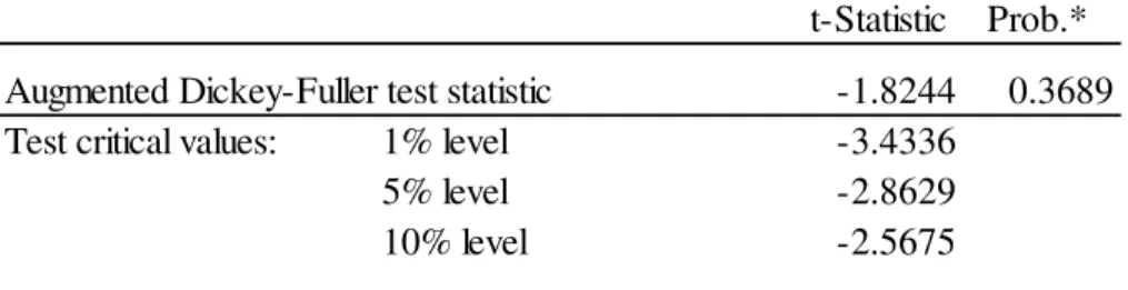
Table 11 Augmented Dickey-Fuller Unit Root Test on TURKEY_CDS5Y Null Hypothesis: TURKEY_CDS5Y has a unit root

Exogenous: Constant

Lag Length: 3 (Automatic based on SIC, MAXLAG=25)

t-Statistic Prob.*

Augmented Dickey-Fuller test statistic -1.8244 0.3689

Test critical values: 1% level -3.4336

5% level -2.8629

10% level -2.5675

*MacKinnon (1996) one-sided p-values.

Table 12 Augmented Dickey-Fuller Unit Root Test on EUROBOND Null Hypothesis: EUROBOND has a unit root

Exogenous: Constant

t-Statistic Prob.*

5% level -2.8629

10% level -2.5675

output, associated critical values, and in this case, the p-value: The Augmented Dickey-Fuller (ADF) statistic values and the associated one-sided p-values. Additionally, output reports the critical values at the 1 percent, 5 percent and 10 percent levels. For each table the statistic values are greater than the critical values so that the null hypothesis has not been rejected at conventional test sizes (Hayashi, 2000). The ADF unit root test results for the first difference of variables used in this study as below tables. Output tables (Table 16-20) show that first difference of Turkey’s 5 year CDS, Turkey Eurobond, ISE 100, Dow Jones and FX Basket variables have

(32)

22

no unit root. Therefore the null hypothesis that states that these variables have a unit root has been rejected.

Table 13 Augmented Dickey-Fuller Unit Root Test on ISE_100 Null Hypothesis: ISE_100 has a unit root

Exogenous: Constant

t-Statistic Prob.*

5% level -2.8629

10% level -2.5675

Table 14 Augmented Dickey-Fuller Unit Root Test on DOW_JONES Null Hypothesis: DOW_JONES has a unit root

Exogenous: Constant

t-Statistic Prob.*

5% level -2.8629

10% level -2.5675

After the results of Augmented Dickey-Fuller Test, logarithm and 1st difference levels of variables are taken and used for the rest of the analysis. Therefore, growth rate of the variables will be used for all analysis studied on rest of thesis. Equation of growth ratio calculation is as below:

1

log( ) log(_t _t )

(33)

23

Table 15 Augmented Dickey-Fuller Unit Root Test on FX_BASKET Null Hypothesis: FX_BASKET has a unit root

Exogenous: Constant

t-Statistic Prob.*

5% level -2.8629

10% level -2.5675

Table 16 Augmented Dickey-Fuller Unit Root Test on TURKEY_CDS5Y Null Hypothesis: D(TURKEY_CDS5Y) has a unit root

Exogenous: Constant

t-Statistic Prob.*

5% level -2.8629

10% level -2.5675

Table 17 Augmented Dickey-Fuller Unit Root Test on EUROBOND Null Hypothesis: D(EUROBOND) has a unit root

Exogenous: Constant

t-Statistic Prob.*

5% level -2.8629

10% level -2.5675

(34)

24

Table 18 Augmented Dickey-Fuller Unit Root Test on ISE_100 Null Hypothesis: D(ISE_100) has a unit root

Exogenous: Constant

t-Statistic Prob.*

5% level -2.8629

10% level -2.5675

Table 19 Augmented Dickey-Fuller Unit Root Test on DOW_JONES Null Hypothesis: D(DOW_JONES) has a unit root

Exogenous: Constant

t-Statistic Prob.*

5% level -2.8629

10% level -2.5675

Table 20 Augmented Dickey-Fuller Unit Root Test on FX_BASKET

Null Hypothesis: D(FX_BASKET) has a unit root Exogenous: Constant

t-Statistic Prob.*

5% level -2.8629

10% level -2.5675

(35)

25

Descriptive statistics and correlation results of growths ratios are given below:

Table 21 Descriptive Statistics of Growth Ratios of Variables

Proper Name Number of

Observations Mean

Standard

DCDS5Y 1895 -0.0006 0.0362 0.2646 -0.2709

DEurobond 1895 -0.0003 0.0129 0.1558 -0.1124

DISE100 1895 0.0008 0.0217 0.0894 -0.1007

DDow Jones 1895 0.0000 0.0133 0.1051 -0.0820

DFx Basket 1895 0.0002 0.0091 0.0553 _-0.0904

Table 22 Correlations among Growth Ratios of Variables

DCDS5Y DEurobond DISE100 DDow Jones DFx Basket

DCDS5Y 1.0000

DEurobond 0.6233 1.0000

DISE100 -0.4928 -0.4088 1.0000

DDow Jones -0.3024 -0.2229 0.1032 1.0000

DFx Basket 0.1108 0.1061 -0.0553 -0.0012 _1.0000

Original time series’ charts and their stationary series’ charts are given in Figure 8. 0 200 400 600 800 1000 1200 1400 1600 2002 2003 2004 2005 2006 2007 2008 2009 TURKEY - CDS5Y -200 -100 0 100 200 300 2002 2003 2004 2005 2006 2007 2008 2009 D_TURKEY_CDS5Y

(36)

26 6 7 8 9 10 11 12 13 14 15 2002 2003 2004 2005 2006 2007 2008 2009 EUROBOND -1.2 -0.8 -0.4 0.0 0.4 0.8 1.2 1.6 2002 2003 2004 2005 2006 2007 2008 2009 D_EUROBOND 0 10000 20000 30000 40000 50000 60000 2002 2003 2004 2005 2006 2007 2008 2009 ISE - 100 -4000 -3000 -2000 -1000 0 1000 2000 3000 4000 2002 2003 2004 2005 2006 2007 2008 2009 D_ISE_100 6000 7000 8000 9000 10000 11000 12000 13000 14000 15000 2002 2003 2004 2005 2006 2007 2008 2009 DOW JONES -800 -400 0 400 800 1200 2002 2003 2004 2005 2006 2007 2008 2009 D_DOW_JONES

(37)

27 1.2 1.3 1.4 1.5 1.6 1.7 1.8 1.9 2.0 2.1 2002 2003 2004 2005 2006 2007 2008 2009 FX BASKET -.20 -.15 -.10 -.05 .00 .05 .10 .15 2002 2003 2004 2005 2006 2007 2008 2009 D_FX_BASKET

Figure 8 Graphs for non-stationary and stationary time series (continuing)

2.4 REGRESSION ANALYSIS

In order to understand the relationship between CDS spreads and financial indicators that were introduced in previous section, two variable and multivariable regressions will be used.

A scattergram is a visual representation of the relationship among variables. It uses a two dimensional graph where the values of dependent, or y variable, are on the vertical axis, and those of the independent, or x variable, are on the horizontal axis. The basic property indicated by a scatter gram is whether there is a positive or negative relationship between variables. In a two variable regression below, equation estimated for several variable pairs that include Turkey 5Y CDS.

1 2.

y=c +c x+ ε (2.4.1)

In two variable models it is assumed that there is a linear relationship between series. There may be a more sophisticated relationship between financial variables but the purpose of this analysis is understanding the basic relationship and whether the relationship is positive or negative. In order to estimate parameters the Ordinary Least Squares (OLS) process is used. OLS

(38)

28

process in simple terms minimize sum of square errors (Maravall & Gomez, 2004).

Regression analysis results from Eviews, includes some additional statistical parameters. These parameters are R2, adjsuted-R2, standard error of the regression (S.E. of regression), sum-of-squared residuals, log likelihood, Durbin-Watson statistic, mean and standard deviation (S.D.) of the dependent variable, Akaike Information Criterion (AIC), Schwarz Criterion (SC), F-Statistic (Maravall & Gomez, 2004).

An important property of R-squared (R2) is that it is a nondecreasing function of the number of explanatory variables or regressors present in the model; as the number of regressors increases, R2 almost invariably increases and never decreases. Stated differently, an additional x variable will not decrease R2. In the two-variable regression, the variability of the dependent variable or total sum of squares (TSS) can be separate into explained sum of

squares (ESS) and residual sum of squares (RSS). R2 could be measured in

following equation: 2 ESS R TSS = 2 2 1 1 i i RSS TSS y ε = − = −

∑

(2.4.2)

To further analyze the importance of added variable to a regression, there is a measure known as the adjusted coefficient of determination, or adjusted-R2. The importance of adjust-R2 is, R2, must go up if a variable with any explanatory power is added to the regression. Consequently, a relatively high R2 may reflect the impact of a large data set of independent variables rather that how well the set explains the dependent variable. Adjusted-R2 could be indicated in the following expression:

2 2 1 1 (1 ) 1 n adjusted R R x n k − − = − − − − (2.4.3)

(39)

29

Where the k is the number of independent variables and n is the number of observations, whenever there is more than one independent variable, adjusted-R2 is less than or equal to R2 (Maravall & Gomez, 2004).

The standard error of the regression is a summary measure based on the estimated variance of the residuals. The standard error of the regression is computed as: ' ( ) s T k ε ε = − _(2.4.4)

The sum-of-squared residuals can be used in a variety of statistical calculations, and is presented separately:

2 1 ' T ( _i _i'. ) t y x b ε ε = =

_∑

− (2.4.5)

Eviews reports the value of the log likelihood function (assuming normally distributed errors) evaluated at the estimated values of the coefficients. Likelihood ratio tests may be conducted by looking at the difference between the log likelihood values of the restricted and unrestricted versions of an equation. Results from Eviews do not ignore constant terms. The log likelihood is computed as:

[1 log(2 ) log( ' / )] 2

T

l= − + π + ε ε T

(2.4.6)

The Durbin-Watson (DW) statistic measures the serial correlation in the residuals. The statistic is computed as:

2 2 1 2 1 ( ) / T T t t t t t DW ε ε− ε = = =

∑

−

∑

(2.4.7)

As a rule of thumb, if the DW is less than 2, there is evidence of positive serial correlation. The DW statistic in our output is very close to one,

(40)

30

indicating the presence of serial correlation in the residuals (Maravall & Gomez, 2004).

The mean and standard deviation of y are computed using the standard formula: 1 / T t t y y T = =

_∑

; 2 1 ( ) /( 1) T y t t s y y T = =

_∑

− − (2.4.8)

The Akaike Information Criterion (AIC) is often used in model selection for non-nested alternatives smaller values of the AIC are preferred. For example, the length of a lag distribution can be chosen by choosing the specification with the lowest value of the AIC. AIC is computed as:

2 / 2 /

AIC= − l T+ k T _(2.4.9)

The Schwarz Criterion (SC) is an alternative to the AIC that imposes a larger penalty for additional coefficients:

2 / ( log ) /

SC= − l T+ k T T _(2.4.10)

The F-statistic reported in the regression output is from a test of the hypothesis that all of the slope coefficients (excluding the constant, or intercept) in a regression are zero. For ordinary least squares models, the F-statistic is computed as:

2 2 /( 1) (1 ) /( ) R k F R T k − = − − _(2.4.11)

Under the null hypothesis with normally distributed errors, this statistic has an F-distribution with k− numerator degrees of freedom and T1 − k denominator degrees of freedom. The p-value given just below the F-statistic, denoted probability (F-statistic), is the marginal significance level of the F-test. If the p-value is less than the significance level you are testing, say 0.05, you reject the null hypothesis that all slope coefficients are equal

(41)

31

to zero. For the example above, the p-value is essentially zero, so the null hypothesis could be rejected that all of the regression coefficients are zero. test is a joint test so that even if all the t-statistics are insignificant, the F-statistic can be highly significant.

Wald test used to test the joint significance of coefficients. In this study related to the relationship, Wald test examined whether all coefficients are jointly equal to zero. If slope coefficient in regression analysis is not equal to zero, this means there could be a positive or negative relationship between variables.

Table 23 Regression Output Table Turkey CDS 5Y-ISE100 Dependent Variable: DTURKEY_CDS5Y

Method: Least Squares

Sample (adjusted): 3/22/2002 1/22/2010 Included observations: 1895 after adjustments DTURKEY_CDS5Y=C(1)+C(2)*DISE_100

Coefficient Std. Error t-Statistic Prob.

C(1) 0.0001 0.0007 0.1200 0.9045

C(2) -0.8212 0.0333 -24.6418 0.0000

R-squared 0.2429 Mean dependent var -0.0006

Adjusted R-squared 0.2425 S.D. dependent var 0.0362

S.E. of regression 0.0315 Akaike info criterion -4.0742

Sum squared resid 1.8829 Schwarz criterion -4.0683

Log likelihood 3,862.2830 Durbin-Watson stat 1.9777

The regression estimation results show that there is a negative relationship between Turkey CDS 5Y and ISE 100 variables. According to t-statistics and probability values above, calculated coefficient is statistically significant. This result inline with our priori expectation there should be a negative relationship between these variables. If Istanbul Stock Exchange Index is higher, Turkish Credit Default Swap spread should be lower.

(42)

32

The scatter gram indicates that there is a negative relationship between ISE 100 and Turkey CDS 5Y growth variables. One interpretation of the graph could be that as investors start to buy Turkish stocks, therefore this means Turkey CDS spread in another term default probability should be lower.

-.12 -.08 -.04 .00 .04 .08 .12 -.3 -.2 -.1 .0 .1 .2 .3 DTURKEY_CDS5Y D IS E _ 1 0 0 DISE_100 vs. DTURKEY_CDS5Y

Figure 9 CDS-ISE 100 Scatter

Table 24 Regression Output Table Turkey CDS 5Y-Dow Jones

Dependent Variable: DTURKEY_CDS5Y Method: Least Squares

Sample (adjusted): 3/22/2002 1/22/2010 Included observations: 1895 after adjustments DTURKEY_CDS5Y=C(1)+C(2)*DDOW_JONES

C(1) -0.0006 0.0008 -0.7806 0.4352

C(2) -0.8233 0.0597 -13.8008 0.0000

(43)

33

The regression estimation results show that there is a negative relationship between Turkey CDS 5Y and Dow Jones Index. According to t-statistics and probability values above, calculated coefficient is statistically significant.The adjusted R2 value of 0.0914 means approximately 9 percent of the variation in Turkey CDS 5Y is explained by variation in Dow Jones Index. Since adjusted R2 at most can be 1, the regression line of these two parameters, which is shown in Figure 10, does not fit our data extremely well; as could be seen from that figure the actual data points are not very tightly clustered around the estimated regression line. But coefficient that is significantly different from zero gives a signal about the relationship which is the main purpose of this study.

-.12 -.08 -.04 .00 .04 .08 .12 -.3 -.2 -.1 .0 .1 .2 .3 DTURKEY_CDS5Y D D O W _ J O N E S DDOW_JONES vs. DTURKEY_CDS5Y

Figure 10 CDS-Dow Jones Scatter

The regression estimation results show that there is a positive relationship between Turkey CDS 5Y and FX basket variables. According to t-statistics and probability values above, calculated coefficient is statistically significant.The adjusted R2 value of 0.0117 means that only 1 percent of the variation in Turkey CDS 5Y is explained by variation in Fx Basket. This might seem a rather low value, but typically one obtains low R2 values, possible because of the diversity of the units in data.

(44)

34

Table 25 Regression Output Table Turkey CDS 5Y-Fx Basket Dependent Variable: DTURKEY_CDS5Y

Sample (adjusted): 3/22/2002 1/22/2010 Included observations: 1895 after adjustments DTURKEY_CDS5Y=C(1)+C(2)*DFX_BASKET

C(1) -0.0007 0.0008 -0.8279 0.4078

C(2) 0.4402 0.0908 4.8484 0.0000

This shows, heteroscedasticity should be studied on.

In Figure 11 there is a slightly increasing regression line which is inline with regression positive coefficient result.

-.12 -.08 -.04 .00 .04 .08 -.3 -.2 -.1 .0 .1 .2 .3 DTURKEY_CDS5Y D F X _ B A S K E T DFX_BASKET vs. DTURKEY_CDS5Y

(45)

35

Table 26 Regression Output Table Turkey CDS 5Y-Eurobond Dependent Variable: DTURKEY_CDS5Y

Sample (adjusted): 3/22/2002 1/22/2010 Included observations: 1895 after adjustments DTURKEY_CDS5Y=C(1)+C(2)*DEUROBOND

C(1) -0.0001 0.0007 -0.0987 0.9214

C(2) 1.7573 0.0507 34.6837 0.0000

The regression estimation results show that there is a positive relationship between Turkey CDS 5Y and Eurobond. According to t-statistics and probability values above, calculated coefficient is statistically significant. The adjusted R2 value of 0.3882 means approximately 39 percent of the variation in Turkey CDS 5Y is explained by variation in Eurobond. This result inline with priori expectation that says there should be positive relationship between these variables. If Eurobond yield is higher, Turkish Credit Default Swap spread should be higher also.

Figure 12 indicates that there is a positive relationship between Eurobond and Turkey CDS 5Y growth variables. Another interpretation of the graph could be that as investors start to buy Turkish Eurobonds, Eurobond’s price will increase and yield will decrease, therefore Turkey CDS spread should be lower. Investors will have more incentive to buy Turkish Eurobond with lower default probability which directly related to lower CDS spreads.

(46)

36 -.3 -.2 -.1 .0 .1 .2 .3 -.12 -.08 -.04 .00 .04 .08 .12 .16 DEUROBOND D T U R K E Y _ C D S 5 Y DTURKEY_CDS5Y vs. DEUROBOND

Figure 12 CDS-Eurobond Scatter

Table 27 Multivariate Regression Output Table Dependent Variable: DTURKEY_CDS5Y Method: Least Squares

Sample (adjusted): 3/22/2002 1/22/2010 Included observations: 1895 after adjustments

DTURKEY_CDS5Y=C(1)+C(2)*DEUROBOND+C(3)*DFX_BASKET +C(4)*DISE_100+C(5)*DDOW_JONES

C(1) 0.0002 0.0006 0.2612 0.7939

C(2) 1.3115 0.0522 25.1050 0.0000

C(3) 0.1812 0.0660 2.7459 0.0061

C(4) -0.4709 0.0301 -15.6301 0.0000

C(5) -0.4614 0.0461 -10.0086 0.0000

Log likelihood 4228.4180 Durbin-Watson stat 2.2809

The regression estimation results show that multivariate regression has the biggest adjusted R-squared and Log likelihood measures. This shows additional parameters increased variables power to explain CDS spreads.

(47)

37

Above equation tells us that holding other variables constant, increasing the Eurobond growth rate by 1 point, CDS spread growth by increase 1.31 point. Also, holding other variables constant, increasing the DISE_100 and Ddow_Jones variables will decrease the CDS 5Y spread growth rate. Multivariate analysis results are inline with single variable regression results in terms of coefficients. Based on output table it is clear that Eurobond and Fx Basket have positive relationship with Turkey CDS 5Y. But ISE 100 and Dow_Jones variables have negative relationship. According to t-statistics and probability values in Table 27, calculated coefficients are statistically significant. -.12 -.08 -.04 .00 .04 .08 .12 -.3 -.2 -.1 .0 .1 .2 .3 DTURKEY_CDS5Y D IS E _ 1 0 0 -.12 -.08 -.04 .00 .04 .08 -.3 -.2 -.1 .0 .1 .2 .3 DTURKEY_CDS5Y D F X _ B A S K E T -.12 -.08 -.04 .00 .04 .08 .12 .16 -.3 -.2 -.1 .0 .1 .2 .3 DTURKEY_CDS5Y D E U R O B O N D -.12 -.08 -.04 .00 .04 .08 .12 -.3 -.2 -.1 .0 .1 .2 .3 DTURKEY_CDS5Y D D O W _ J O N E S

(48)

38 Table 28 Wald Test

Wald Test: Equation: Untitled

Test Statistic Value df Probability

F-statistic 446.3994 (4, 1891) 0.0000

Chi-square 1,785.5980 4.0000 0.0000

Null Hypothesis Summary:

Normalized Restriction (= 0) Value Std. Err.

C(1) 1.3113 0.0522

C(2) 0.1816 0.0659

C(3) -0.4707 0.0301

C(4) -0.4615 0.0461

Restrictions are linear in coefficients.

The low probability values indicate that the null hypothesis that C(1)=0, C(2)=0, C(3)=0, C(4)=0 is strongly rejected. Therefore, there is a relationship between Turkey CDS 5Y and financial indicators analyzed.

2.5 GRANGER CAUSALITY TESTS

To simplify the analysis assume there are two time series of interest, which are denoted y and _t x . The central idea is that _t y is not Granger caused by _t

t

x if the optimal predictor of y_t does not use information from x_t. In applications of this idea the predictor is usually restricted to be an optimal linear predictor and optimality is defined as minimizing the mean squared error of the h-step predictor of y_t. To be specific suppose y_t and x_t have a

vector autoregressive (VAR) representation in which y depends upon lags _t

of itself and lags of xt and symmetrically xtdepends upon lags of itself and lags ofy_t (Patterson, 2000). If y_t is weakly exogenous for α and, in addition, x_t does not Granger cause y_t, then y_t is said to be strongly

(49)

39

exogenous for α. Granger causality or non causality is concerned with whether lagged values of y_t do or do not improve on the explanation of y_t obtainable from only lagged values of xt itself (Granger, 1969).A simple test is to regress y_t on lagged values of itself and lagged values of x_t (2.5.1). If the latter are jointly insignificant, x_t is said not to Granger cause

t

y . If one or more lagged xt values are significant then xt are said to Granger cause y_t (2.5.2). The test, however, is often very sensitive to the number of lags included in the specification. Changing lag length can result in changed conclusions. If strong exogeneity holds, β may be estimated from the conditional distribution alone and used to make forecasts of x_t conditional on forecasts of y_t, the latter in turn being derived from the past history of y_t alone ( Johnston & Dinardo, 1997).

0 1 1 ... 1 1 ... 1 t t p t p t p t p t y =α +α y− + +α y− +βx− + +β x− +ε (2.5.1) 0 1 1 ... 1 1 ... 2 t t p t p t p t p t x =α +α x− + +α x− +β y− + +β y− +ε (2.5.2)

Before Grange Causality analysis, the number of lagged terms to be introduced in the causality tests is an important practical question (Hamilton, 1994). The result of proper number of lags is as follow.

FPE and AIC give lag 3 as compatible number of lags. On the other hand, HQ gives lag 2 and SC gives lag 1. Since AIC was chosen in stationary tests before, lag length criteria will also be chosen for analysis. For this model lag length will be 3. The results are as follows: the null hypothesis in each case is that the variable under consideration does not “Granger cause” the other variable.

(50)

40 Table 29 Determining Compatible Number of Lags

VAR Lag Order Selection Criteria

Endogenous variables:DTURKEY_CDS5Y DDOW_JONES DEUROBOND DFX_BASKET DISE_100

Exogenous variables: C Sample: 3/21/2002 1/22/2010 Included observations: 1883

Lag LogL FPE AIC SC HQ

0 26121.91 6.17E-19 -27.73968 -27.72497 -27.73426 1 26971.06 2.57E-19 -28.61503 -28.52676* -28.58252 2 27052.01 2.42E-19 -28.67446 -28.51263 -28.61486* 3 27091.75 2.39E-19* -28.69012* -28.45472 -28.60342 4 27108.55 2.41E-19 -28.68141 -28.37246 -28.56762 5 27125.64 2.43E-19 -28.67301 -28.29049 -28.53213 6 27150.00 2.43E-19 -28.67233 -28.21625 -28.50435 7 27177.41 2.42E-19 -28.67489 -28.14525 -28.47982 8 27204.27 2.42E-19 -28.67686 -28.07366 -28.45471 9 27227.18 2.42E-19 -28.67464 -27.99788 -28.42539 10 27255.85 2.41E-19 -28.67855 -27.92822 -28.40220 11 27279.63 2.42E-19 -28.67724 -27.85336 -28.37381 12 27309.92 2.40E-19 -28.68287 -27.78542 -28.35234

* indicates lag order selected by the criterion FPE: Final prediction error

AIC: Akaike information criterion SC: Schwarz information criterion HQ: Hannan-Quinn information criterion