Protein-protein interaction network alignment using GPU

KADIR HAS UNIVERSITY

GRADUATE SCHOOL OF SCIENCE AND ENGINEERING

PROTEIN-PROTEIN INTERACTION NETWORK ALIGNMENT

USING GPU

MOHAMMAD SOHAIB

D S O H A IB M as te r T he sis 20 16

PROTEIN-PROTEIN INTERACTION NETWORK ALIGNMENT

USING GPU

MOHAMMAD SOHAIB

B.E., Information Communication Systems, National University of Sciences and Technology, Pakistan. 2014

M.S., Computer Engineering, Kadir Has University, 2016

Submitted to the Graduate School of Science and Engineering In partial fulfillment of the requirements for the degree of

Master of Science In Computer Engineering

KADIR HAS UNIVERSITY May, 2016

KADIR HAS UNIVERSITY

GRADUATE SCHOOL OF SCIENCE AND ENGINEERING

PROTEIN-PROTEIN INTERACTION NETWORK ALIGNMENT USING GPU

MOHAMMAD SOHAIB

APPROVED BY:

Assoc. Prof. Zeki BOZKUŞ Kadir Has University _______________ (Thesis Supervisor)

Asst. Prof. Tamer DAĞ Kadir Has University ________________

Assoc. Prof. Ahmet Yücekaya Kadir Has University ________________

i

PROTEIN-PROTEIN INTERACTION NETWORK ALIGNMENT

USING GPU

Abstract

The alignment of Protein-Protein Interaction Networks is becoming an imperative phenomenon in Bio-Informatics that leads to several vital results. These results can be used in numerous fields associated with Bio-Informatics including the prediction/variation of evolutionary relationships, finding cures for gene inflicted diseases (like cancer) and identifying probable therapies. However, with the introduction of fast sequencing and other technologies that spawn large amounts of data for computing (since the proteins are very large in size and have many nodes and edges), limiting dynamics arise. These include performance, scalability and time consumption. Recently, CPU versions of the alignment procedures and computations have been introduced. However, because of the large size of the proteins, they are very time-consuming. Therefore, in this thesis, I propose a GPU version for performing the computations quickly and efficiently. This thesis is based on improving the efficiency of SPINAL, a polynomial time heuristic algorithm introduced by [1] that finds the similarities between pairs of PPI-Networks. In this thesis, the sequential algorithm of SPINAL is converted into a parallel algorithm using Heterogeneous Programming Library (HPL) that performs the computations in a massively parallel fashion on a single GPU with 448 thread processors, a clock rate of 1.15 Giga Hertz and 6 Giga Bytes of DRAM. The modifications/enhancements to the algorithm result in a significant speedup as compared to the benchmark algorithms.

Keywords: Protein-Protein Interaction Networks, Graphics Processing Unit, Scalable Protein Interaction Network Alignment, Parallel Programming, Heterogeneous Programming Library.

ii

GPU KULLANARAK PROTEIN – PROTEIN ETIKILESIM AĞI

HIZALAMA

Özet

Protein protein etkileşim ağı hizalama problemi biyo-informatikte pek çok önemli çözüme öncülük eden kaçınılmaz problemlerden biridir. Bu sonuçlar biyo-informatikle alakalı, evrimsel ilişkiler, kanser gibi gen ile alakalı hastalıklar ve muhtemelen terapilerin bulunması gibi pek çok konuyla ilişkilidirler. Buna ragmen, programlama için çok yüksek miktarda veri ortaya çıkaran hızlı dizilimler ve diğer teknolojiler (proteinler çok büyük olduklarından ve pek çok düğüm ve linke sahip olduklarından) bu alanda sınırlı kalmaktadırlar. Bu performans, ölçeklenebilirlik ve zaman tüketimini ilgilendirir. Alignment yöntemleri ve hesaplamalarının CPU versiyonları mevcuttur. Ama proteinlerin büyüklükleri nedeniyle çok zaman alıcıdırlar. Bu sebepten, bu tezde, hızlı ve etkili işlem yapan bir GPU versiyonunu sundum. Bu tez [1] tarafından geliştirilmiş SPINAL isimli PPI-Ağları çiftleri arasındaki benzerliği bulan bir polynomial time heuristic algoritmasının daha etkili hale getirilmesine dayalıdır. Bu tezde seri olarak yazılmış SPINAL, Heterogeneous Programming Library (HPL) kullanılarak paralel bir algoritmaya dönüştürülmüştür. HPL ile yoğun paralel işlem yapabilen 1.15 Ghz’de çalışan 6 GB DRAM içeren tek bir GPU’da 448 süreç işlemcisinden faydalanılmıştır. Ölçümlerden anlaşıldığı üzere algoritmadaki düzenlemeler ve geliştirmeler ciddi hızlanmaya sebep olmuştur.

Anahtar Sözcükler: Protein-Protein Etkileşim Ağı, Grafik İşleme Birimi, Ölçeklenebilir Protein Etkileşim Ağları Dizilemesi, Paralel Programlama, Heterojen Programlama Kütüphanesi

iii

Acknowledgements

First and foremost, I would like to take this opportunity to express my gratitude and special thanks to my supervisor, Assoc. Prof. Zeki Bozkus, who supported me throughout the project and thesis period. I am extremely indebted to him for his guidance and supervision.

I would also like to extend my sincere thanks to Assoc. Prof Cesim Erten for his kind support in teaching me how the algorithm works and which part to target for my thesis.

In addition, I would like to thank: Teodora and Serkan, for their assistance in making me grasp the concept of Proteins, their interactions and the biological aspect of this thesis; Syazz, for getting me through many difficult situations with her humor; Abdul Ahad and Abdur Rehman, for always being there for me whenever I needed help; my family, for believing in me and supporting me throughout this process. And of course my mom, for her incredible support and unconditional love and prayers – no thesis without her.

iv

Table of Contents

PROTEIN-PROTEIN INTERACTION NETWORK ALIGNMENT USING GPU ... i

Abstract ... i Özet. ... ii Acknowledgements ... iii Table of Contents ... iv List of Tables ... v List of Figures ... vi

List of Abbreviations ... vii

Introduction ... 1

1.1. Thesis Structure ... 4

Overview of SPINAL ... 5

2.1. The Algorithm: ... 5

2.2. Array Based Solution: ... 7

Performing SPINAL on GPU ... 10

3.1 GPU Architecture ... 10

3.2 OpenCL: ... 13

3.3 HPL: ... 16

3.4 Performing SPINAL on GPU ... 17

v

Results ... 23

4.1 Processing and Analyzing Results ... 23

4.2 Explaining Results Using Amdahl’s Law: ... 25

Related Works ... 27 Conclusion ... 29 References ... 31 Curriculum Vitae ... 35

List of Tables

vi

List of Figures

vii

List of Abbreviations

PPI Protein-Protein Interaction

HPL Heterogeneous Programming Library

GPU Graphics Processing Unit

CPU Central Processing Unit

DNA Deoxyribonucleic Acid

RNA Ribonucleic Acid

NBG Neighborhood Bipartite Graph

LEDA Library of Efficient Data-types and Algorithms SPINAL Scalable Protein Interaction Network Alignment

ILP Instruction Level Parallelism

SIMD Single Instruction Multiple Data

ALU Arithmetic Logic Unit

SM Streaming Multiprocessor

OpenCL Open Computing Language

FPGA Field Programmable Gate Arrays

OpenMP Open Multi Processing

1

Chapter 1

Introduction

The DNA (Deoxyribonucleic Acid) is a self-replicating substance that is present in approximately all living organisms as the fundamental constituent of chromosomes. It is also the carrier of genetic information. The DNA is a linear sequence of four nucleotides. When necessary, the DNA is translated into RNA (Ribonucleic Acid). The RNA acts as a messenger that takes instructions from the DNA and carries out those instructions for the synthesis of proteins.

Figure 1: Translation of DNA into RNA and then into Proteins.

Proteins are made up of amino acid chains and are the focal machinery of the cell. They perform functions that are as complex as the functions of DNAs and RNAs. They are among the primary macromolecular players of the cell. They comprise of one or more extended chains of amino acids residues. Their functions include, but are not limited to, DNA replication, responding to stimuli, catalyzing metabolic reactions, and transporting molecules from one location to another. Proteins are also in charge of cell growth, nutrient uptake and morphology.

2

Figure 2: A Simple protein.

Proteins bind with each other via a number of combinations of salt bridges, hydrophobic bonding, and Van der Waals. These bindings occur at certain binding domains on each protein. The sizes of the domains can vary from small binding clefts to large surfaces. Also, they could be a few peptides long or spam hundreds of amino acids. The size of the binding domain impacts the strength of the binding.

Protein-Protein Interactions take place when two or more proteins come in contact with each other as a result of bio-chemical events and/or electrostatic forces. Proteins typically act in groups. The PPIs organize a large number of proteins components and build molecular machines that carry out many processes inside a cell. The “interactions-system” of a living cell is reliant on the interactions of these proteins. Whereas, abnormal interactions are the source of many diseases (including cancer and Alzheimer’s disease).

Even though the data on PPI Networks is developing steadily, thorough understanding of the “interaction surfaces” and their dynamics still remains partial. Currently available PPI-Networks, or also known as “interactome maps”, acquired with the high-tech methods of the new era, only cover a very small portion of the entire PPI-Networks. In these partial networks, only a few proteins have a large number of

3

interaction partners. The rest of them rarely participate in any interactions [2]. Many researches and methodologies have been formulated to map PPI-Networks from different species onto each other to find out the similarities between them [3]. These similarities are useful for performing and formulating several other methodologies in the Bio-Informatics world which include, but are not limited to, finding cures and potential therapies for gene inflicted diseases [4]. The mapping of different PPI-Networks onto each other is also knows as alignment.

Figure 3: Simple Protein-Protein Interaction Network. The circles depict the proteins, while the lines between then represent the edges (or interactions) between the proteins. Several alignment techniques have been proposed and executed. In this thesis, I will propose a modified algorithm for SPINAL (Scalable Protein Interaction Network Alignment) which was proposed by [1]. The modification is twofold: the first modification corresponds to converting the LEDA graph into simple array based structures; and the second one is implementing the algorithm using HPL (Heterogeneous Programming Language) performed on GPUs.

Since GPUs use massively parallel architecture, the alignment algorithm runs much faster even for very large proteins. In [1], one of the major issues is the consumption of the algorithm. Since the algorithm is defined only for CPUs, the time-consumption problem increases with some input PPI Networks containing tens of

4

thousands of nodes and edges. With their algorithm, they have improved the trade-off between accuracy and scalability, but even then, the algorithm takes a very long time to execute. Therefore, we propose an optimum solution for the algorithm based on GPUs. Our algorithm optimizes the performance and increases the scalability while keeping the accuracy at an optimum level in hopes to provide solutions and answers to the users in a much faster way.

1.1. Thesis Structure

This thesis has two main parts. The first part is an overview of SPINAL that was proposed by [1], explanation of the algorithm and an array based solution to simplify and speed up the algorithm.

Overview of SPINAL. Explanation of the algorithm. Array based solution.

The second part is about implementing the algorithm using HPL (Heterogeneous Programming Language) on a GPU. It consists of a little bit of introduction to GPUs and Heterogeneous Programming, OpenCL and HPL. And then our solution to make the algorithm parallel.

GPUs and Heterogeneous Programming OpenCL

HPL

5

Chapter 2

Overview of SPINAL

Provided a pair of PPI-Networks from two different species, a pair-wise global alignment relates to the one-to-one mapping among their proteins. Assuming that pairs of functionally orthologous proteins are delivered precisely by such mappings, the outcomes of the alignment may then be used in comparative systems biology problems such as function verification/prediction or creation of evolutionary relations.

[1] has provided a polynomial time heuristic algorithm, SPINAL, which consists of two main phases. The first one is coarse-grained alignment phase where all pairwise initial similarity scores are constructed. The next phase is fine-grained phase where the final one-to-one mapping is performed by iteratively growing a locally improved solution. For this thesis, I will concentrate only on improving the first phase, i.e. the course-grained alignment phase.

2.1. The Algorithm:

Let PPI-1 = (V1, E1) and PPI-2 = (V2, E2), be two networks where V1 and V2 correspond to the set of the nodes in the proteins and E1 and E2 correspond to the set of edges or interactions in the proteins. In the coarse-grained alignment, each node (V1) of PPI-1

has a number of neighboring nodes that correspond to the neighbors of another node

(V2) selected from PPI-2. The coarse grained alignment method keeps the score of the neighborhood pairs that have higher weight in another list and disregards the rest. It grows a list this way by iteratively going through each node of PPI-1 and compares it to each node of PPI-2. In the end, we get a neighborhood bipartite graph that has the maximum weights.

6

Figure 4: SPINAL global alignment algorithm.

Here, in Figure 4, we can observe that for each node of V1 and each node of V2, a neighborhood bipartite graph (NBG) is produced that depicts the maximum-weight similarity matrix between all the nodes of PPI-1 and PPI-2. Then a contributor set C

7

Figure 5: Equation for alignment (SPINAL).

In SPINAL, the initial coarse-grained alignment phase is the one where more than 95 of the execution time is spent. The reason is because of the use of LEDA libraries for the execution of several graph/node related computations such as adding/deleting nodes etc. But that in turn proves to increase the execution time drastically. So we propose to make that crucial part, where the coarse-grained alignment takes place, LEDA-free. For that, we introduce simple arrays and HPL based arrays, both equally important, instead of LEDA nodes and lists. The usage of arrays gives us many advantages including better memory utilization which LEDA fails to achieve.

2.2. Array Based Solution:

Arrays are a collection of the identical types of elements stored in a contiguous memory location. It is index based. Meaning the first element is stored at 0th index, the second element at 1st index and so on.

Figure 6: Representation of an array of length 5 in memory.

8

To declare a simple array of length 5 of type integer, the following syntax is used: int array[5];

To access a specific element (let’s say third) in an array, the following syntax is used: int item = array[2];

Converting the LEDA dependent graphs into simple arrays was my first step towards modification of the algorithm. The conversions from LEDA dependent graphs and nodes was applied from step 3 till step 14 in Figure 4. The benefit of using arrays is that they are stored in contiguous memory locations unlike LEDA nodes. They are easily accessible and there is no overhead when accessing the next element of the array. We used arrays instead of LEDA nodes and edges. Copied the values of these nodes and edges and neighboring nodes of each node from the LEDA structures to arrays.

The code iterates over all the nodes of PPI-1 and each node of PPI-1 iterates over all the nodes of PPI-2. The purpose of these iterations is to find the best similarity between the nodes of PPI-1 and PPI-2. We also created arrays of Tuples that have three values. The first value depicts the index of the first node from PPI-1, the second value represents the number of the second node from PPI-2 and the third value represents the score or the interaction value between them. This Tuple is iteratively updated until it finds the maximum weighted node pair from the two PPI-Networks (the nodes with the highest score).

9

Figure 7: Algorithm for collecting "heavy" neighbor pairs in tuples

Then we applied a simple bubble sort method on the Tuples that we got and created sorted arrays which helps us easily figure out the Tuples with the highest and lowest scores for selection and elimination respectively. And then after a few more minor operations, we update the scores of the nodes that are calculated using the equation from Figure 5. We loop through this whole procedure several times until we get the best similarity scores.

Since arrays are more memory efficient and the whole block is placed in one memory space together, just by changing the LEDA arrays into simple arrays drastically improved the performance of the program. All the nodes of the pairs of the PPI-Networks were converted into arrays. At this stage, no significant changes were made to the algorithm. And just because of this small conversion from LEDA to array structures, the algorithm ran much faster than before. The time spent on the crucial part of the algorithm decreased. The results obtained were much better and this lead the path for us to apply parallel programming using HPL on GPUs.

10

Chapter 3

Performing SPINAL on GPU

3.1 GPU Architecture

During the 1990s till early 2000s, there were substantial improvements in gates per die, clock speed and instruction level parallelism (ILP), that helped grow the rate of processor performance exponentially. However, the improvement in clock speed started to hit physical limits due to power consumption and heat effects in 2003. It was revealed that CPUs can’t get any faster. On the other hand, transistors kept on shrinking, which led to an increase in the transistor density (also known as gate count) on a single chip. Consequently, many manufacturers have reconfigured their improvement strategy to focus on gate count instead of pushing clock rate, in particular to making more cores (C. Boyd, Data-Parallel Computing, ACM Queue, vol. 6, no. 2, pp. 30-39, 2008.) and [5].

Afterwards, the processor chips were brought into parallel systems that are now regarded as multicore CPUs and many-core GPUs. In these systems, the cores are populated with multiple floating-point arithmetic logic units (ALUs), where each ALU performs the same operation on distinct pieces of data. Hence the parallelization of computations performed on a large data set, also known as SIMD (Single Instruction Multiple Data) approach. The architecture consists of a CPU and its own memory (Host), GPU part and the GPUs memory (the Device). Furthermore, the GPU consists of a set of a large number of streaming multi-processors (SMs). Each SM contains:

• Thousands of registers • Several caches.

11 • Warp schedulers. • Dispatch units. • Execution cores. • Control Units • Local Memory Figure 8: The architecture of a GPU. The arrows define the flow/transfer of data between the host (CPU) and the device (GPU).

The SMs are general-purpose processors, but they are designed very differently than the execution cores in CPUs: they target much lower clock rates; they support instruction-level parallelism. Whereas, branch prediction or speculative execution is not supported; and they have a smaller amount of cache, if any at all. For codes that deal with massive amounts of data that needs to be parallelized, the CPU allocates a chunk of memory to hold the data and then copies the data onto the GPUs memory. Then, according to the programmers needs, the GPU divides the data between

12

different streaming multiprocessors. Each SM performs the same operation on a different chunk of data. Furthermore, the SMs can access the global memory and their own memory (local memory), but cannot access any other SMs memory. After all the instructions have been executed, the results are copied back to the CPU memory. This whole process can also be defined as offloading compute-intensive portions of the application to the GPU, while the remainder of the code still runs on the CPU.

Figure 9: Architecture of a Streaming Multiprocessor.

GPUs nowadays have thousands of cores to process parallel workloads efficiently due to their massively parallel architecture and they are increasing day by day. They are extremely good for data parallelization. They can also perform task parallelization, but are not as efficient.

13

3.2 OpenCL:

OpenCL (Open Computing Language) is a standard for programming a vast variety of heterogeneous platforms. These platforms are built from Graphics Programming Units (GPUs), Field Programmable Gate arrays (FPGAs), as well as Central Processing Units (CPUs), and many other processors and hardware accelerators. OpenCL is a C99-based programming language used for programming compute devices. When different types of processors are available in a single system, programmers can write task-parallel and/or data-parallel programs taking advantage of the processors. The main objective of OpenCL is to empower the programmer to use all the computational resources in the system.

Explaining the anatomy of OpenCL; it has two main parts. The first one is the serial code which executes on the host. The serial code part is responsible for allocating and creating buffers for various variables including arrays that are to be sent to the device. The main purpose of this code is to prepare the data in proper OpenCL format to be sent into the device through a command queue. The command queue manages executions of kernels and accepts various commands including: kernel execution commands, synchronization commands and memory commands. The second part is the kernel code that is the basic executable code which runs on OpenCL devices. The code can either be data-parallel or task-parallel. This is the part where multiple kernels run concurrently [6].

The memory model of OpenCL can be described in the following manner:

• Global Memory: Visible and accessible to all the kernels. Can be read and written to by any thread. Therefore, needs careful implementation.

14

• Constant Memory: Read only by kernels/threads. They do not have permission to write. Host can only read and write this kind of memory.

• Local Memory: Read and written by only the kernels/threads in the same work-group.

• Private Memory: Only accessible to one kernel/thread.

Figure 10: OpenCL host side code for preparing the devices, context, command queue and kernel etc. Figure 11: OpenCL host code for creating input and output arrays in device for calculation. Figure 12: A Simple OpenCL kernel side code that returns squares of the elements.

15

Figure 13: Memory Model of OpenCL

As you can see from the above code snippets (Figure 10, 11 and 12), OpenCL requires a lot of work. It requires the programmers to select the devices, create contexts, create a command queue that will en-queue and de-queue commands, compute the kernel etc. Along with this, there are a lot of other requirements to be met before a programmer can execute his code on the device. These include creating memory buffers for the data in the device. Copying the values from host to the device memory. Building the program info and then executing the kernel. It also has a special syntax for getting the results returned by the device.

16

3.3 HPL:

HPL (Heterogeneous Programming Library) enhances the programmability of heterogeneous systems. At the same time, it allows lower level control to the programmer and provides performance synonymous to the likes of lower level approaches. The underlying architecture is mostly based on OpenCL, therefore, the memory model is the same between the two.

HPL uses a two key concepts:

• Arrays: special data-types that can be programmed in both the host side and the device side. They follow a special syntax format:

Array<type, ndim [, memoryFlag]>

Where “type” represents the normal standard of C++ contents. “ndim” represents the dimensions of the array. And “memoryFlag” (optional) represents one of the memory kinds that is supported (Global, Local or Constant).

Figure 14: Simple declaration of Arrays in HPL

17

Figure 15: Simple 'kernel' call in HPL using “eval”

The code inside the kernels can be written both in OpenCL C format as well as in any C++ embedded language provided by HPL. The library is responsible for converting the latter format into OpenCL, which enables execution on a variety of devices. The programmers are required to define all the data types and structures, which is to be used in the kernels, as HPL Arrays [7].

Unlike OpenCL, the programmer does not have to get the device ids or the memory context from the system. Neither does the programmer have to create memory buffers at the kernel for the data to be copied into the device. All these operations are handled by the HPL itself. The programmer just needs to declare arrays in proper HPL format and just call the kernel function using these arrays. The rest is HPL’s job. This is one of the reasons why it is much easier to code than OpenCL.

3.4 Performing SPINAL on GPU

HPL (Heterogeneous Programming Language) is based on OpenCL, therefore, most of the underlying architecture is the same between the two. The main difference is the tradeoff between performing more complicated work and being easily programmable.

18

OpenCL is complex and it gives programmers a lot of options on how to handle the data and memory etc. but is quite difficult to program since it requires programmers to allocate simple C based arrays and structures and then allocate memory buffers for these arrays so they can be sent to the device. On the other hand, HPL is easily programmable with just a few restrictions. HPL also doesn’t require the copying back of results that are obtained from the device side code (kernel code). Whereas, OpenCL requires special syntax and programming rules to be followed to copy back results from device to host and many other operations.

SPINAL is programmed on CPU using LEDA library. The reason for using LEDA is that it makes certain operations on the nodes of the PPI networks easy, for example; adding new nodes, deleting nodes, etc. But the problem is poor utilization of memory space. The different nodes are placed in different parts of the memory and with each iteration to the next node, it has to jump to a new memory location to fetch the node attributes (e.g. number of neighbors, weight etc.), which makes the program run very slow and most of the time is spent in this part. The first main change we brought into the SPINAL program was that we converted the LEDA dependent PPI networks and nodes etc. into array based elements, since HPL can work only on simple C/C++ arrays. By doing so, each PPI network was represented by an array (e.g. PPI-1, PPI-2, neigh_ppi-1, neigh_ppi-2 etc.) and each element of the array represented a node. Since arrays are more memory efficient and the whole block is placed in one memory space together, just by changing the LEDA arrays into simple arrays drastically improved the performance of the program.

After that crucial part of the program (that took 95 percent of the running time) was LEDA free, not only were we able to improve the time consumption, we also were able to apply OpenMP. OpenMP uses the many cores of the CPU. E.g. if a CPU has

19

4 cores, it breaks down the block, that it is applied to, into 4 smaller parts and assigns each CPU one part, so we get a 4-fold improved performance.

After that, we created the required HPL arrays that use different notation than normal C/C++ arrays. We created other important HPL variables. And then called the “eval” function and passed the important HPL variables and arrays to it, such as 1, PPI-2, neigh_ppi-1, neigh_ppi-2 etc.

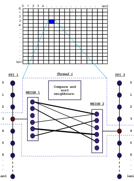
Figure 16 is representation of how each thread works. We have two arrays of len1 and

len2 where arrays represent the network of PPI-1 and PPI-2 respectively. Each element of the arrays corresponds to the nodes. Each element in itself has a number of neighbors where range of the number of neighbors is:

R where (0 <= R <= max (len1 or len2))

And this list is being kept in different arrays. The lines of same length between the elements of PPI-1 and PPI-2 represent the interactions within the nodes of the networks. Whereas, the lines that are of different widths among the neighbors of V1 and V2 represent the interaction/ similarities between the neighbors of V1 and the neighbors of V2. The different widths represent the different scores of the interactions. We create len1 * len2 threads where each thread is responsible for comparing a node V1 from PPI-1 to another node V2 from PPI-2 based on the similarities between their neighbors.

20

Figure 16: Graphical Representation of how Threads handle the PPI-Network arrays.

21

The weights of the neighbors of V1 are calculated with respect to the neighbors of V2, only the corresponding neighbors that have the highest weights between them are considered, whereas the rest, if present, are discarded. By doing so, the neighboring elements of V1 have an almost one-to-one mapping with the neighboring elements of

V2. This method is repeated for each node of PPI-1 and PPI-2 several times until enough iterations. Each thread performs comparison and sorting operations on the respective neighbors of each node. We then construct a NBG/array such that they are of the neighbors that have the highest weight/similarity score between them and the graph/comparison becomes almost a one-to-one mapping.

3.4.1 Implementation Details

One of the difficulties in writing programs with OpenCL language is the lack of “malloc()” (short for “memory allocation”) routine in the kernel code that runs on the GPU. Unfortunately, our application requires a variety of dynamic data structures such as linked lists, dictionaries and variable size arrays.

We developed a two level strategy to solve this problem. First, we used static data structures in the kernel. If the graph vertexes construct a small neighbor lists, this may waste some valuable memory space but this may be acceptable since this path is only chosen for small sizes. Next, we allocated a fixed number of data structures in the device memory before kernel executions and we shared this fix number of data structure resources among many kernels by relying on mutual exclusion (mutex) locks of access to shared resources.

Figure 17: Implementation of `mutex` locks.

22

In the current implementation, we have used 100 mutex locks to guard 100 data structures to allow 100 kernels to run concurrently. Our application has a potential

len1 * len2 total of parallelism. There is almost no limitation for concurrent computations with available processing elements (PE) of GPU. However, GPU system memory cannot handle this much memory if each kernel requires a large memory. By using mutex locks, we are constraining device memory usage such that we could run the application on the GPU. Otherwise too much parallelism may consume too much memory and we may not be able to run our application because of the lack of memory resources.

23

Chapter 4

Results

SPINAL was implemented in C++ using LEDA [8], and was experimented on data from four different species: Saccharomyces cerevisiae, Drosophila melanogaster, Caenorhabditis elegans and Homo sapiens. I applied my algorithm on the same four species and examined two kinds of results. First one is the estimated time taken for the algorithm to run. Or also known as time-consumption. The second one is the accuracy of the results. Or in other words, how close our scores were to the scores obtained from SPINAL.

4.1 Processing and Analyzing Results

Time consumed for running the algorithm was drastically decreased after we removed all the LEDA dependencies and introduced and used simple C arrays instead. As explained earlier, LEDA places different nodes in different parts of the memory and with each iteration to the next node, it has to jump to a new memory location. It makes certain node operations (including node addition and deletion) easy. But it consumes a lot of time. This was the first milestone that we achieved. Just by converting the LEDA dependent algorithm into simple arrays, we got a maximum speed up of around 40%. Though it is not visible for pairs of PPI-Networks with comparatively a smaller number of nodes, such as ce-dm (Caenorhabditis elegans - Drosophila melanogaster), ce-hs (Caenorhabditis elegans - Homo sapiens) and ce-sc (Caenorhabditis elegans - Saccharomyces cerevisiae). It is more evident for the results of larger pairs of PPI-Networks like dm-hs (Drosophila melanogaster - Homo sapiens) and dm-sc (Drosophila melanogaster - Saccharomyces cerevisiae).

24

Data Set SPINAL

(Time) (Score) ARRAYS (Time) (Score) HPL (Time) (Score) ce-dm 8m 15s 2310 5m33s 2369 1m 52s 2015 ce-hs 11m 45s 2277 8m 38s 2318 2m 30s 2057 ce-sc 9m 34s 2288 8m 1s 2341 1m 40s 1918 dm-hs 41m 1s 5825 22m 6s 5894 8m 54s 0 dm-sc 31m5s 5229 17m 39s 5322 6m 54s 5078 Table 1: Comparison between the original algorithm (SPINAL), after conversion to simple ARRAYS and HPL

After we got the results from simple arrays, we implemented the algorithm using HPL. We used a Tesla C2050/C2070 GPU as our experimental platform. The device has 448 thread processors with a clock rate of 1.15 GHz and 6GB of DRAM and it is connected to a host system consisting of 4xDual-Cores Intel 2.13 GHz Xeon processors. With HPL, we got a drastic decrease in the time consumption. The parallelization of the algorithm gave us 4-5 times speed up. But on the other hand, the resulting scores were not very good. Still, they were close to the original scores. For very large sized PPI-Networks, such as dm-hs (Drosophila melanogaster - Homo sapiens), we got a result of 0. Which means the device was not able to handle such a large amount of threads.

25

Figure 18: Time Consumption Comparison between SPINAL, ARRAYS and HPL

4.2 Explaining Results Using Amdahl’s Law:

Amdahl’s law is used to discover the maximum enhancement in a complete system when only a portion of the system has been enhanced. In heterogeneous programming, this law is used to find out the maximum improvement in the speedup after some part of the code has been improved (parallelized). The equation for Amdahl’s law is:

𝑠𝑝𝑒𝑒𝑑𝑢𝑝 = 1

1 − 𝑝𝑎𝑟𝑎𝑙𝑙𝑒𝑙 𝑐𝑜𝑑𝑒 + 𝑝𝑎𝑟𝑎𝑙𝑙𝑒𝑙 𝑐𝑜𝑑𝑒_{𝑡𝑖𝑚𝑒𝑠 𝑓𝑎𝑠𝑡𝑒𝑟}

Where ‘parallel code’ represents the portion of code out of on part that can be made parallel and ‘times faster’ represents the number of concurrent processors (ideal speedup). 0 5 10 15 20 25 30 35 40 45

ce-dm ce-hs ce-sc dm-hs dm-sc

Time Consumption of Algorithms (in minutes)

26

If we apply Amdahl’s law to our system, we get the following results:

𝑠𝑝𝑒𝑒𝑑𝑢𝑝 =

4 5 6.89 : ;.<=₌

=

6.69 : 6.48

= 4.16

And for finding the percentage improvement: 100 1 −_?@AABC@4 = 76 %

So theoretically, we should get an improvement of this much percent. But then again there are some parts which cannot be completely parallelized. Also a lot of other computations, such as copying to and from the original LEDA arrays occur. That is why it take a bit longer than expected and the speedup is a bit low.

27

Chapter 5

Related Works

The information obtained from the alignment of PPI networks can be used in identification and study of new genes and their properties, identifying disease related sub-networks and network based disease classification [4]. It can also be used in predicting functions of proteins with unknown functions or in verifying those with known functions [9]; [10] or in reconstructing evolutionary dynamics. Several methods/algorithms have been formulated and implemented for aligning PPI-Networks. These include PathBLAST [11]; NetworkBLAST [12], MaWISH [13], Graemlin [14], Graph match and split algorithm [15] that use the local network alignment where sub-networks that closely match each other both in terms of network topology and/or sequence similarities are identified.

In Global Network Alignment, the networks are aligned as a whole rather than focusing on sub-networks. The recent GNA techniques include ISORank [10], PATH and GA [16], PISwap [17], MIGRAAL [18], NATALIE, NetAlignBP, NetAlignMR, [19], [20], [21]. [1] shows that the problem is NP-Hard even for the case where the pair of networks are simply paths. It further provides a polynomial time heuristic algorithm, SPINAL, where the first phase is to construct all pairwise initial similarity scores and then employ these scores to achieve the final one-to-one mapping by iteratively growing a locally improved subset. Our contribution are based on the works of [1] where it was suggested to align the networks globally, providing unambiguous one-to-one mappings between the proteins of different networks.

[22] uses a parallel algorithm for clustering PPI-Networks based on the parallel implementations of Girvan and Newmann (Girvan and Newman 2002). [23] uses

28

parallel architectures and procedures to implement general clustering algorithms for large scale biological data sets using MPI. Fast parallel Markov clustering [24] uses GPU computing based on CUDA implementation to perform parallel sparse matrix-matrix computations and parallel sparse Markov matrix-matrix normalizations one of the most popular open source modular and distributed system that processes datasets by using parallel computing approaches.

29

Conclusion

In this thesis, we present a GPU based solution for the alignment of Protein-Protein Interaction Networks. Our work is based on the algorithm implemented by [1] known as SPINAL. Firstly, we have provided some insight into the creation and functionality of proteins. Then, the mechanism of how proteins interact with each other and combine to form large strands. Then, the characteristics of Protein-Protein Interactions is described. Then, the working and algorithm of SPINAL is explained. Afterwards, our solution to speed up the algorithm is provided.

The solution is twofold. First, converting the LEDA dependent graphs into simple C based arrays. And then implementing the GPU part using HPL. We get a decrease of 40% in time consumption just after converting LEDA dependent graphs into arrays. Then we get even a much better result with HPL.

The scores (results) obtained from array based implementation are good and acceptable. They are quite close to the scores obtained from SPINAL. The problems occur with HPL. Though we get a very good speedup (approximately 8 times faster with some pair of PPI-Networks), the resulting scores are close to the ones obtained by SPINAL, but not very good. With the massively parallel computations that we are performing on the GPU, it is very easy to generate errors. For example: for a pair of two very large arrays of sizes approximately around 5000 and 7000, we are creating (5000 * 7000) threads. Some GPUs might not be able to handle these many threads. Others might handle them but not properly. Working on such large PPI-Networks is a very complex operation.

As a further research, the large arrays (PPI-Networks) could be broken down into smaller arrays and then sent to the GPU one by one. And then their results should be

30

collected in the end. This way the GPUs don’t have to handle an extremely large number of threads.

31

References

[1] A. E. Aladaǧ and C. Erten, “SPINAL: Scalable protein interaction network alignment,” Bioinformatics, vol. 29, no. 7, pp. 917–924, 2013.

[2] H. Kitano, “Computational systems biology.,” Nature, vol. 420, no. 6912, pp. 206–10, 2002.

[3] N. Krasnogor and D. A. Pelta, “Measuring the similarity of protein structures by means of the Universal Similarity Metric,” Bioinformatics, vol. 20, no. 7, pp. 1015–1021, 2004.

[4] T. Ideker and R. Sharan, “Protein networks in disease,” Genome Research, vol. 18, no. 4. pp. 644–652, 2008.

[5] G. Chen, G. Sun, Y. Xu, and B. Long, “Integrated research of parallel computing: Status and future,” Chinese Sci. Bull., vol. 54, no. 11, pp. 1845– 1853, 2009.

[6] J. E. Stone, D. Gohara, and G. Shi, “OpenCL: A parallel programming standard for heterogeneous computing systems,” Comput. Sci. Eng., vol. 12, no. 3, pp. 66–72, 2010.

[7] M. Vi??as, Z. Bozkus, and B. B. Fraguela, “Exploiting heterogeneous parallelism with the Heterogeneous Programming Library,” J. Parallel Distrib. Comput., vol. 73, no. 12, pp. 1627–1638, 2013.

[8] K. Mehlhorn and S. Näher, “LEDA: a platform for combinatorial and geometric computing,” Commun. ACM, vol. 38, no. 1, pp. 96–102, 1995.

32

eukaryotes.,” BMC Bioinformatics, vol. 10, p. 393, 2009.

[10] R. Singh, J. Xu, and B. Berger, “Global alignment of multiple protein interaction networks with application to functional orthology detection.,” Proc. Natl. Acad. Sci. U. S. A., vol. 105, no. 35, pp. 12763–12768, 2008.

[11] B. P. Kelley, B. Yuan, F. Lewitter, R. Sharan, B. R. Stockwell, and T. Ideker, “PathBLAST: A tool for alignment of protein interaction networks,” Nucleic Acids Res., vol. 32, no. WEB SERVER ISS., 2004.

[12] M. Kalaev, M. Smoot, T. Ideker, and R. Sharan, “NetworkBLAST: Comparative analysis of protein networks,” Bioinformatics, vol. 24, no. 4, pp. 594–596, 2008.

[13] M. Koyutürk, Y. Kim, U. Topkara, S. Subramaniam, W. Szpankowski, and A. Grama, “[10] Pairwise alignment of protein interaction networks.,” J. Comput. Biol., vol. 13, no. 2, pp. 182–99, 2006.

[14] J. Flannick, A. Novak, B. S. Srinivasan, H. H. McAdams, and S. Batzoglou, “Gr??mlin: General and robust alignment of multiple large interaction networks,” Genome Res., vol. 16, no. 9, pp. 1169–1181, 2006.

[15] M. Narayanan and R. M. Karp, “Comparing protein interaction networks via a graph match-and-split algorithm.,” J. Comput. Biol., vol. 14, no. 7, pp. 892– 907, 2007.

[16] M. Zaslavskiy, F. Bach, and J.-P. Vert, “A path following algorithm for the graph matching problem,” Pattern Anal. Mach. Intell. IEEE Trans., vol. 31, no. 12, pp. 2227–2242, 2009.

33

[17] L. Chindelevitch, C. Y. Ma, C. S. Liao, and B. Berger, “Optimizing a global alignment of protein interaction networks,” Bioinformatics, vol. 29, no. 21, pp. 2765–2773, 2013.

[18] O. Kuchaiev and N. Pržulj, “Integrative network alignment reveals large regions of global network similarity in yeast and human,” Bioinformatics, vol. 27, no. 10, pp. 1390–1396, 2011.

[19] Z. Liang, M. Xu, M. Teng, and L. Niu, “NetAlign: a web-based tool for comparison of protein interaction networks.,” Bioinformatics, vol. 22, no. 17, pp. 2175–7, 2006.

[20] B. Dost, T. Shlomi, N. Gupta, E. Ruppin, V. Bafna, and R. Sharan, “QNet: a tool for querying protein interaction networks.,” J. Comput. Biol., vol. 15, no. 7, pp. 913–925, 2008.

[21] A. McKenna, M. Hanna, E. Banks, A. Sivachenko, K. Cibulskis, A. Kernytsky, K. Garimella, D. Altshuler, S. Gabriel, M. Daly, and M. A. DePristo, “The genome analysis toolkit: A MapReduce framework for analyzing next-generation DNA sequencing data,” Genome Res., vol. 20, no. 9, pp. 1297–1303, 2010.

[22] Q. Yang and S. Lonardi, “A parallel edge-betweenness clustering tool for Protein-Protein Interaction networks,” Int J Data Min Bioinform, vol. 1, no. 3, pp. 241–247, 2007.

[23] M. Wang, W. Zhang, W. Ding, D. Dai, H. Zhang, H. Xie, L. Chen, Y. Guo, and J. Xie, “Parallel clustering algorithm for large-scale biological data sets,” PLoS One, vol. 9, no. 4, 2014.

34

[24] A. Bustamam, K. Burrage, and N. A. Hamilton, “Fast parallel markov clustering in bioinformatics using massively parallel computing on GPU with CUDA and ELLPACK-R sparse format,” IEEE/ACM Trans. Comput. Biol. Bioinforma., vol. 9, no. 3, pp. 679–692, 2012.

35

Curriculum Vitae

Mohammad Sohaib was born on February 14th, 1990, in Peshawar, Pakistan. He received his BE in Information Communication Systems, in 2014 from National University of Sciences and Technology, Pakistan. From 2013 to 2014, he worked in a startup company as an Android Application Developer. Since March, 2016, he is working as a back-end programmer for Polizom, a startup company in Turkey.