INQUIRING the MAIN ASSUMPTION of the ASSEMBLY LINE
BALANCING PROBLEM: SOLUTION PROCEDURES USING
AND/OR GRAPH
A THESIS
SUBMITTED TO THE DEPARTMENT OF INDUSTRIAL ENGINEERING AND THE INSTITUTE OF ENGINEERING AND SCIENCE
OF BILKENT UNIVERSITY
IN PARTIAL FULFILLMENT OF THE REQUIREMENTS FOR THE DEGREE OF
MASTER OF SCIENCE
By Ali Koç July 2005
I certify that I have read this thesis and that in my opinion it is fully adequate, in scope and in quality, as a thesis for the degree of Master of Science.
Prof. İhsan Sabuncuoğlu (Principal Advisor)
I certify that I have read this thesis and that in my opinion it is fully adequate, in scope and in quality, as a thesis for the degree of Master of Science.
Prof. Erdal Erel
I certify that I have read this thesis and that in my opinion it is fully adequate, in scope and in quality, as a thesis for the degree of Master of Science.
Assoc. Prof. Selim Aktürk
Approved for the Institute of Engineering and Science:
ABSTRACT
Inquiring The Main Assumption Of The Assembly Line Balancing
Problem: Solution Procedures Using And/Or Graph
Koç, Ali
M.S. in Industrial Engineering Supervisor: Prof. İhsan Sabuncuoğlu
July 2005
In this thesis, we consider the assembly/disassembly line balancing (ADLB) problem. The studies in the literature consider assembly and disassembly problems separately and use task precedence diagram (TPD) and AND/OR Graph (AOG) in assembly and disassembly line balancing problems, respectively. In contrast to these studies, we use AOG for both assembly and disassembly line balancing problems, considering these two problems as complementary of each other. Hence, we call the complementary problem as ADLB-AOG. We show theoretically that AOG is a more general version of the TPD. We also develop integer programming (IP) and dynamic programming (DP) formulations to solve the ADLB-AOG problem. Our analysis indicates that the DP formulation performs much better than the IP formulation in terms of the problem sizes that can be optimally solved. We also develop a DP-based heuristic to solve large-size instances of the ADLB-AOG problem. An experimentation of the procedures on some sample problems and the implementation of the heuristic on a sample problem are also given.
Keywords: Assembly, Disassembly, Line Balancing, AND/OR Graph, Task Precedence Diagram, Integer Programming, Dynamic Programming, Heuristic.
ÖZET
Montaj Hattı Dengeleme Problemlerının Temel Varsayımını Sorgulama: And/Or
Grafiği Kullanılarak Geliştirilen Çözüm Prosedürleri
Ali Koç
Endüstri Mühendisliği Yüksek Lisans Tez Yöneticisi: Prof. İhsan Sabuncuoğlu
Temmuz 2005
Bu tezde, montaj/demontaj hattı dengeleme problemini incelemekteyiz. Literatürdeki çalışmalar, montaj ve demontaj problemlerini ayrı ayrı olarak ele alıp montaj hattı dengeleme problemi için iş önceliği diyagramını, demontaj hattı dengeleme problemi için ise AND/OR grafiğini kullanmaktadırlar. Biz ise her iki problemi birbirinin tersi olarak ele aldığımız için, her ikisinde de AND/OR grafiğini kullandık. Binaen aleyh, problemi montaj/ demontaj hattı dengeleme problemi olarak isimlendirdik. Ayrıca, teorik olarak ta gösterdik ki AND/OR grafiği, iş önceliği diyagramından daha genel olduğundan bu grafik kullanılarak çözülen problem diğerinden daha iyi, en azından aynı, neticeler vermektedir. Öne sürülen bu problemi hem tamsayı programlama hem de dinamik programlama yöntemleri ile çözdük. Bu iki yöntemle bazı örnek problemleri çözdüğümüzde, dinamik programlama yöntemi inkar edilemez bir farkla tamsayı programlama yöntemini geride bıraktı. Daha büyük problemlerin çözebilmesi için daha hızlı çalışan bir sezgisel yöntem de geliştirdik. Tüm problem verileri, örnek çözümler ve uygulamaları, gerek metnin içinde gerek ilave bölümlerde verilmiştir.
Anahtar Kelimeler: Montaj, Demontaj, Hat Dengeleme, AND/OR Grafiği, İş Önceliği Diyagramı, Tamsayı Programlama, Dinamik Programlama, Sezgisel Yöntem.
TABLE OF CONTENTS
CHAPTERS
INTRODUCTION ... 1
1.1MOTIVATION... 1
1.2STATEMENT OF THE PROBLEM AND RELATED CONTRIBUTION... 3
LITERATURE SURVEY ... 6
2.1BACKGROUND... 6
2.2LITERATURE SURVEY... 13
PROPOSED THEORY: QUESTIONING THE FUNDAMENTAL ASSUMPTIONS AND SOLVING THE ACTUAL PROBLEM ... 16
3.1AND/ORGRAPH AND ASSEMBLY/DISASSEMBLY TREE... 17
3.1.1 AND/OR Graph (AOG)... 17
3.1.2 Assembly/Disassembly Tree (AT/DT) ... 19
3.2THEOREM OF SUB-OPTIMALITY... 24
3.3THE DERIVATION OF A TPD FROM THE AOG... 29
3.4AN EXAMPLE TO COMPARE TPD AND AOG. ... 36
THE SOLUTON TO THE ADLB-AOG PROBLEM ... 40
4.1THE PROPOSED DYNAMIC PROGRAMMING (DP)FORMULATION... 42
4.1.1 Definitions and Terminology ... 42
4.1.1.1 Partial AOG’s...42
4.1.1.2 Assembly task sequences ...43
4.1.1.3 Relation between partial AOG’s and assembly task sequences...45
4.1.2 The Proposed DP Approach ... 45
4.2.1 The Formulation ... 53
4.2.2 Example ... 56
4.3SOLVABLE SIZES OF ADLB-AOG PROBLEM BY DP AND IP METHODS... 57
4.3.1 The DP formulation ... 61
4.3.2 The IP Formulation ... 70
4.4ADP BASED HEURISTIC... 73
CONCLUSIONS AND FUTURE RESEARCH DIRECTIONS ... 78
REFERENCES ... 81
AND/OR GRAPH AND RELATED CONCEPTS IN ASSEMBLY / DISASSEMBLY PROCESS PLANNING ... 90
A1.1ASSEMBLY... 90
A1.2ASSEMBLY TASK... 92
A1.3ASSEMBLY SEQUENCE... 96
A1.4DISCUSSION ON AOG ... 97
FIGURES OF THE EXAMPLE 2 IN SECTION 3.3 ... 106
FIGURES OF THE EXAMPLE 3 IN SECTION 3.3 ... 122
STORING AOG IN A MATRIX... 136
SOME EXAMPLES TO PARTIAL AOG (AOG(S))... 138
JAVA CODE FOR THE DP METHOD TO THE ADLB-AOG PROBLEM ... 142
JAVA CODE FOR THE FORMULATION OF ADLB-AOG PROBLEM AS PURE 0-1 IP PROGRAMMING ... 154
JAVA CODE TO GENERATE AOG... 158
LİST OF FİGURES
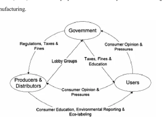
Figure 1 Interaction between government, users, producers and distributors as the driving force of the
environmental management (taken from Gungor and Gupta 1999)... 8
Figure 2 Environmental management practices and their environmental contributions... 9
Figure 3 Different post-life options for the relinquished products ... 11
Figure 4 Remanufacturing and demanufacturing as the means of reverse manufacturing ... 12
Figure 5 A sample product (de Mello and Sanderson (1990))... 17
Figure 6 AND/OR Graph of the Product in Figure 5 ... 18
Figure 7 All of the 8 DT’s obtained from the AOG in Figure 2 ... 22
Figure 8 Eight transformed disassembly trees (TDT) associated with the eight DT’s in Figure 4... 24
Figure 9 Theorem of sub-optimality... 28
Figure 10 The subassemblies of AOG in Figure 6, their GOC and corresponding tasks ... 32
Figure 11 The m AT S obtained from SAT in Figure 8 ... 33
Figure 12 STPD obtained by combining equitask ATm’s in Figure 11 ... 34
Figure 13 Transformed AND/OR Graph of the AOG in Figure A.14 of Appendix 3 ... 41
Figure 15 The partial AOG’s obtained while solving the example problem ... 51
Figure 16 Dynamic programming solution to the ADLB-AOG problem for the AOG in Figure 14 . 52 Figure 17 Sample AOG’s to illustrate the experimentation... 59
Figure 18 Solvable problem sizes when the number of tasks for each artificial node is 1 ... 64
Figure 19 Solvable problem size when the number of tasks for each artificial node is 2... 64
Figure 20 Solvable problem size when the number of tasks for each artificial node is 3... 65
Figure 21 Solvable problem size when the number of tasks for each artificial node is 5... 65
Figure 23 The solution duration vs. difficulty of the problem... 71
Figure 24 Solution of a sample problem by the DP method... 73
Figure A.1 Graph of connections (GOC) for the product in Figure 5 of Chapter 2... 91
Figure A.2 A feasible assembly sequence (τ1, τ2, τ3) ... 94
Figure A.3 An infeasible assembly sequence (τ1, τ4, τ5) ... 95
Figure A.4 A loosely connected product, its graph of connections and AOG... 101
Figure A.5 A strongly-connected product, its graph of connections and AOG ... 102
Figure A.6 Proposed AND/OR graph... 105
Figure A.7 An example product and its GOC (Lambert 1999) ... 106
Figure A.8 AOG of the product in Figure A.7 ... 107
Figure A.9 SAT established from the AOG in Figure A.8 ... 112
Figure A.10 The subassemblies of AOG in Figure A.8, their GOC and corresponding tasks... 115
Figure A.11 The m AT S obtained from SAT in Figure A.9 ... 120
Figure A.12 STPD obtained by combining equitask ATm’s in Figure A.11 ... 121
Figure A.13 An example product and its GOC (Lambert 1999) ... 122
Figure A.14 AOG of the product in Figure A.13... 123
Figure A.15 SAT established from the AOG in Figure A.14 ... 127
Figure A.16 The subassemblies of AOG in Figure A.14, their GOC and corresponding tasks... 130
Figure A.17 The m AT S obtained from SAT in Figure A.15 ... 134
Figure A.18 STPD obtained by combining equitask ATm’s in Figure A.17 ... 135
Figure A.19 AOG ({A13}) ... 138
Figure A.20 AOG ({A6}) ... 139
Figure A.21 AOG ({A7}) ... 139
Figure A.22 AOG ({A8}) ... 140
Figure A.23 AOG ({A8, A13}) ... 140
LIST OF TABLES
Table 1 Durations of the SD and SI tasks in the example... 37
Table 2 The solutions to the three example problems ... 38
Table 3 Solvable size of the AOG’s without parallelism by the DP approach. ... 62
Table 4 The difficulties of 124 sample problem and solution durations... 69
Table 5 The results of the heuristic solution to the ADLB-AOG problem compared with the exact results of both ADLB-TPD and ADLB-AOG problem. ... 76
C h a p t e r 1
INTRODUCTION
1.1 Motivation
Due to the threatening environmental issues, in recent years, demanufacturing and remanufacturing of products gained an increasing attention from both practitioners and researchers (Grenchus et al. 1997, Spicer and Johnson 2004, Thierry et al. 1995, Ayres et al. 1997, Bras and McIntosh 1999, Guide Jr VDR. 2000, Parkinson and Thompson 2003). Both practices rest mostly on the disassembly of the products. Consequently, disassembly process, ranging from factory level, through work system level, to the operation level, gained a considerable attention from the researchers (Brennan et al. 1994, Kochan 1995, Zussman 1995, Wiendahl et al. 1999, Gungor and Gupta 1999, Tang et al. 2000, Lee et al. 2001, Lambert 2003).
Almost all of the researchers sought ways of handling the disassembly issue independent of the assembly process. Even though disassembly and assembly differ to a great extent due to the differences in production planning and inventory control issues, there is not so much difference as far as the shop floor activities are concerned: In the disassembly process, we take apart what are put together while assembling the product. Hence, some of the researchers view the
Sanderson 1990, 1991a and 1991b). The authors define all possible assembly/disassembly tasks for a product and establish the precedence relations among the tasks. Each possible task definition and corresponding precedence relation is represented by an assembly/disassembly tree (AT/DT). They develop a graph called AND/OR Graph (AOG) that includes all AT/DT’s of a product.
Inspired from the AOG, in this study, we handled the assembly and disassembly processes as complementary of each other. As a result of this, we pinpoint some of the facts that escape from the eyes of many, in assembly studies. For many years, researchers have sought the ways to solve the assembly line balancing problem (ALB). But they did not question the main input to the problem, the task precedence diagram. Task precedence diagram (TPD) shows the precedence relations between the assembly tasks. They consider only one the many feasible definitions of the assembly tasks. Two differently defined sets of tasks for the same assembly/disassembly process yield two different TPD’s. Consequently, the number of stations in the line to assemble/disassemble the same product for different set of tasks may change. Based on this, when balancing the assembly/disassembly line optimally, we use AOG instead of the TPD to consider all possible task definitions. The objective is to minimize the cycle time while keeping the number of stations constant. We showed that using AOG is better than using TPD.
1.2 Statement of the Problem and Related Contribution
Disassembly activities take place in both remanufacturing and demanufacturing practices. Disassembly is a systematic method for separating a product into its constituent parts, components, subassemblies or other groupings (Gupta and Taleb 1994). Assembly may be defined just as the reverse of the disassembly. Even though due to some characteristics of disassembly process, assembly and disassembly should be treated independently, we suggest that, at least for the operational purposes, they should be considered as the complementary of each other. Hence, all the inferences, discussions and results obtained in this study will apply to both assembly and disassembly.
Assembly/disassembly line is made up of an ordered sequence of stations connected by a material handling system. The line may be paced or unpaced. In paced assembly lines, the cycle time for all stations is common, whereas in unpaced lines all stations are allowed to operate at their own phase. In assembly line, parts of the product enter the line and move to the downstream stations until (some of) the parts are assembled. Whereas in disassembly line, the whole product enters the line and moves to the downstream stations until the parts of concern are obtained. Both assembly and disassembly may be partial or complete. In partial assembly, parts are assembled not until obtaining the whole product but until some subassemblies are formed. Similarly, in partial disassembly a product is disassembled to obtain subassemblies of interest. Partial assembly/disassembly is motivated by the profit maximization objective including the time and cost components of the tasks and profit component of the subassemblies, while
complete assembly/disassembly is driven by only the time components of the tasks in the process.
Performing assembly and disassembly require certain apparatus and certain operators. Technological and physical conditions define the precedence relations among the tasks. In this study, we will use AND/OR Graphs (AOG) developed by de Mello and Sanderson (1990) instead of the classical task precedence diagrams (Prenting and Battaglin 1964) used in assembly line balancing (ALB) problems. We also show the superiority of AOG over the classical task precedence diagrams (TPD) in line balancing problems.
The problem in this study may be posed as follows: Assign the assembly/disassembly tasks of a product obtained from the AOG to an ordered sequence of stations in order to completely assemble/disassemble the product, such that the precedence relations in AOG are satisfied and number of stations is minimized for a cycle time common to all stations. We call the problem as assembly/disassembly line balancing problem for AOG (ADLB-AOG). The scarce literature related to the problem is given in chapter two.
One of the major contributions of this study is to show that the common practice over fifty years of finding an optimum solution for the ALB problem using a TPD constitutes an upper bound on the actual problem that should be defined on AOG. In the third chapter, we prove that an assembly/disassembly line balancing problem for the classical task precedence diagram yields an inferior solution to the assembly/disassembly line balancing problem for the AOG. By an example we show the superiority of the AOG over the TPD. We also show how to obtain the TPD from the AOG by three examples in the same chapter. Another
contribution is the development of dynamic programming (DP) and integer programming (IP) approach to the proposed problem. In the fourth chapter we develop these two methods. The IP formulation of the problem was previously given by Altekin (2005). But, the IP formulation proposed there considers not only the AOG but also other precedence diagrams (such as part precedence diagrams) and aims partial disassembly. In contrast, the IP formulation proposed here is more effective in the sense that it is tailored to the specific problem that considers only the complete assembly case and uses only AOG as the precedence relations. Hence, for this problem type, development of suitable IP formulation is another contribution. In the same chapter, we compare the IP and DP formulations in terms of the size of the problem they can handle by generating sample AOG’s defined by three parameters. We also develop a DP based heuristic in this chapter. Finally, we discuss the conclusions and inferences in chapter five.
C h a p t e r 2
LITERATURE SURVEY
Before the literature review, we will give some background information on why the disassembly process is a vital element of the so-called ‘environmentally conscious’ industry. Even though this section can be omitted without loosing the integrity of the study, we recommended reading in order to see how the disassembly studies including the disassembly line balancing are developed. Then, we present the scarce literature of disassembly line balancing problem and refer the interested reader to the milestones of the huge world of assembly line balancing problem.
2.1 Background
By the advent of developments in science and technology, the Earth became an industrial world with all of its resources, both energy and minerals. A plethora of desirable products in the market place, may be more than the demand, and heedless consumption have decreased the natural resources, including air quality, water, mines, diversity of flora and fauna, and most importantly the landscape. Furthermore a series of industrial accidents in 1970s and 1980s, such as the accident at Bhopal in India, the Exon Valdez oil spill, etc., have increased the environmental awareness.
People, oblivious to environmental degradation of industrialization before, began to realize the adversarial effects of the industrial world on the environment. Therefore, there appeared the buzzword green consumerism, which shows people’s reaction as supporting and encouraging the green products and boycotting the others. Government also passed some legislation against the mass production, heedless consumption, indiscriminate disposal habits and polluting hazardous products (Bodily and Gabel, 1982; Bonifant et al. 1995; Klassen and Angell, 1998). What remains to corporations is to obey and comply with the rulings by changing the infrastructural and structural components so that the impacts of the production, usage and disposal of the products on the ecology are appeased (Bodily and Gabel, 1982; Barney, 1991; Corbett and Wassenhove, 1993; Elkington, 1994; Gupta M.C., 1994; Epstein, 1996; Florida, 1996; Azzone et al. 1997; Maxwell et al. 1997; Hart, 1997; Zhang et al. 1997; Hartman and Stafford, 1998; Inmann, 2002).
The endeavor of citizens, government and corporations to alleviate the environmental degradation is called environmental management (EM) (Figure 1). It is defined as the total of the efforts lessening and alleviating the adverse environmental affects of industrialization. Industrialization includes the production and service facilities. The term describing management of both of these practices is called production and operations management (POM) (Gupta MC 1994). Hence, to attain the goal of environmental management, also dubbed as ‘sustainable development’, one should either lessen the hazardous effects of POM activities or decrease the activities itself. To decrease the harmful effects of POM
POM activities, i.e., to increase the production efficiency by serving the same demand with less production, is the focus of closed loop manufacturing (CLM) (Brown and Karagozoglu 1998) (Figure 2). Pollution prevention rescues renewable resources of the nature such as air and water quality, and landscape by abating the hazardous waste releases. Closed loop manufacturing (CLM) includes product design and process design. Product design is the process of designing for environment (DFE), while process design is to establish and coordinate reverse manufacturing (RM) and reverse logistics (RL) activities to take back the post-use products (cores) and reemploy them either by remanufacturing or demanufacturing.
Figure 1 Interaction between government, users, producers and distributors as the driving force of the environmental management (taken from Gungor and Gupta 1999)
Figure 2 Environmental management practices and their environmental contributions
Reverse manufacturing (RM) closes the loop in production processes by reemploying and reutilizing the products, parts and materials that were processed in the past, so that, in the extreme, once spent, natural resources and energy are used forever. Reverse manufacturing is an essential element of closed-loop manufacturing system. It is estimated to be 73,000 firms are engaged in remanufacturing in US, employing 350,000 people (Lund, 1998). Remanufacturing activities amounts to total revenue of $14 billion per year (US Environmental Protection Agency, EPA 2001). As a point of reference, consider the US steel industry has annual sales of $56 billion employing 241,000 people (Lund, 1998).
The automotive industry leads the practice of the reverse manufacturing activities. One example is the Mercedes Benz that decided to implement a recycling program including two elements: design and recycling. What is more,
Pollution Prevention
Core Recovery (Closed Loop Mfg.)
Liquid and gaseous waste reduction to rescue
Decrease in Resource Usage (Energy and Minerals)
Post-use phase
Environmental Contributions New trends in the industry
(magical concepts)
Solid waste reduction Production and
the material content since then (Gungor and Gupta, 1999). Another example is BMW. That gives credit to the customers for turning the used car back. Also, BMW uses color codes for different plastic materials in order to simplify the recycling, and claims producing 90% recyclable cars. Some other firms making similar efforts are General Motors, Volkswagen, Nissan Motor Company and Volvo Car Corporation (Gungor and Gupta, 1999). Deere and Company entered in to an agreement with Springfield Remanufacturing Company that they will recondition diesel engines and components for Deere and Company. Sales of reconditioned engines in 1996 exceeded $2.5 billion dollars (Guide et al. 2000). Computer and peripheral makers, such as IBM, Hewlett Packard, and Xerox, are applying disassembly. Xerox applies remanufacturing for its photocopiers and toner cartridges in US and abroad and estimates a cost saving of $20 million per year (Guide et al. 2000). In 1998, out of 33 power-tool manufacturers 13 of them agreed to take back their products from the customers in Germany (Klausner and Hendrickson, 2000).
The dichotomy that classifies the reverse manufacturing practices into two parts, demanufacturing and remanufacturing, is mainly decided by the different types of treatments to the cores, which we call end-of-life (EOL) options. In the early times before the environmentalism occurred, people were used to get rid of the products without any treatment. Today’s attitude is to reemploy the product as much as possible in order to both reduce municipal solid wastes (MSW) and to lessen the usage of energy and resource. But, still, some relinquished products are disposed. Consequently, when a product completes its lifetime and is relinquished by the consumers, there are mainly two types of treatments: disposal and recovery
(Figure 3). Disposal option is to get rid of the product without any further treatment, which is done mainly in the form of landfilling. Recovery options, on the other hand, reclaim some benefit from the used product. Although the aim in recovery processes is to claim a win-win situation that serves both to the environment and to the budget, some of the recovery options, such as composting, incineration, etc, do not aim environmental friendliness.
Figure 3 Different post-life options for the relinquished products
Since some of the recovery options require no or little treatments, there are two of them, among all, requiring detailed study and research: remanufacturing
Revalorization / recovery
Retain the geometric form of the product
Primary use Secondary use
(The use of tires as mooring cushions)
- Reuse as is - Resell Rebuilding / Renovation:
Remanufacture / refurbish Destroy the geometric
form of the product (Demanufacturing) Recycling, cannibalization, etc - Composting - Incineration - Others - Landfilling
- Illegally tipping storing
components of the product, while demanufacturing is decomposing the product into components so that most profitable end-of-life (EOL) options for each component can be chosen. Remanufacturing focuses on product recovery, whereas demanufacturing, in the form of recycling and cannibalization, focuses on part and material recovery. Hence, remanufacturing closes both material and energy use cycle, while demanufacturing closes only material use cycle (Figure 4). The following quotation from White et al. (2003) makes the distinction between demanufacturing and remanufacturing clear in the computer industry. “The distinction between demanufacturing and remanufacturing, which has not been emphasized in the literature, is a subtle one. As opposed to remanufacturing’s focus on rebuilding products and reclaiming assets in support of forward remanufacturing, demanufacturing operates mostly to divert wastes from disposal and reuse assets wherever practicable.
It is seen that there are two main elements of reverse manufacturing; remanufacturing and demanufacturing. Both of the practices are as important as the manufacturing in the in the environmentally conscious world. Since they both rest heavily on the disassembly, disassembly should be as important as the assembly.
2.2 Literature Survey
Assembly line balancing (ALB) problem attracted a great deal of interest for fifty years (Flood, 1956; Talbot et al. 1986; Scholl and Klein, 1999). Researchers considered the problem of assigning a set of tasks to an ordered set of stations such that the precedence relations between the tasks are maintained and the number of stations is minimized. The main inputs to the assembly line balancing (ALB) studies are the task precedence diagram (TPD) and the durations of the tasks (Salveson, 1955; Held et al. 1962). Both of the inputs depend on how the definitions of the tasks are set. Hence, we believe that the questions of “are there other ways of defining the tasks?” and “how does the duration and precedence of the tasks differ with respect to definitions?” should be of interest. Although there are so many efforts on how to solve the ALB problem, there is little attention on how to define the tasks of the assembly process. The derivation of TPD is typically left to the ‘engineering judgment’ (Chow 1990). In a study by Prenting and Battaglin (1964), authors consider how to define the tasks and how to form the precedence diagram. They list some of the guidelines in ‘element listing’ and ‘diagramming’. But they do not point out the scenario where the solution to
ALB problem changes with respect to the different TPD’s formed by listing the elements in a different way.
As the research in ALB literature goes on, there appeared the new concept of disassembly as a result of the environmental concerns (Brennan et al. 1994; Zhang et al. 1997; Wiendahl et al. 1999; Gungor and Gupta, 1999; Lee et al.2001; Lambert, 2003). Firms, under the pressure of both governments and the NGO’s, began to consider remanufacturing and demanufacturing as the means of profitability. Remanufacturing aims to recover the after-use products, while demanufacturing reemploys the post-use products by means of cannibalization and recycling. Both of them require disassembly process. When the disassembly studies occurred, researchers realized that there is not only a single way of defining tasks, as it was case in ALB studies. Consequently, De Mello and Sanderson (1990, 1991a and 1991b) established a graph that includes all possible assembly/disassembly task sequences of a product, called AND/OR Graph (AOG). Researchers used AOG in disassembly studies instead of TPD (Lambert, 1997, 1999, 2002; Penev and de Ron, 1996; Pnueli and Zussman, 1997; Rai et al. 2002; Johnson and Wang, 1995, 1998).
Disassembly line balancing (DLB) literature is a scarce one. DLB problem is first defined in the study by Gungor and Gupta (2001b and 2002). However, they use neither the TPD nor the AOG in their studies. They use a part precedence diagram (PPD), which was developed in one of their early studies (Gungor and Gupta, 2001a). PPD involves the parts of the product, rather than the tasks. Since most of the researchers devote the TPD to assembly studies, there is no study that uses the TPD in DLB problems. As it will be clear later, there is no reason to not
using the TPD in DLB studies. The only study in this area that uses AOG is by Altekin (2005). The author considers not only the task durations but also task costs and subassembly profits. Hence, it is a profit oriented disassembly line balancing problem, involving costs revenues and planning horizon. The inputs are task durations and costs, subassembly demands and profits and station opening and operating costs. As a result of the solution, it may turn out that the product is fully or completely disassembled. Also, the decision of disassembly leveling may differ from one period to another. The gigantic model developed cannot be solved to optimality. The author develops some heuristic techniques to solve the integer programming formulation of the problem.
C h a p t e r 3
PROPOSED THEORY: Questioning
the Fundamental Assumptions and
Solving the Actual Problem
After the disassembly studies began to draw considerable attention, researchers sought ways to compare and contrast assembly and disassembly. As mentioned in the literature, they usually state that disassembly problem is a more general form of the assembly since they used the AOG in disassembly, whereas only the TPD has been used in assembly studies. We discuss in this chapter that disassembly line balancing (DLB) problem is the reverse of the ALB problem. Furthermore, we prove that AOG is a more general version of TPD and should be used for both of the assembly and disassembly studies, as opposed to many that allocate the former to the disassembly and the latter to the assembly. As a result, both assembly and disassembly line balancing problems for AOG constitutes a lower bound on the same problem for TPD.
In the first section we introduce the concepts of AOG and AT/DT. We then consider the assembly/disassembly line balancing problem (ADLB) for an AOG, denoted AOG, and compare it with the ADLB for a TPD, denoted ADLB-TPD. We prove that the solution to the ADLB-TPD is always an upper bound on
TPD of a product can be obtained from the AOG of the same product. We give two examples on how to obtain a TPD from the AOG. Finally, in the last section, we give an example to illustrate the proposed theory in this chapter.
3.1 AND/OR Graph and Assembly/Disassembly Tree
3.1.1 AND/OR Graph (AOG)
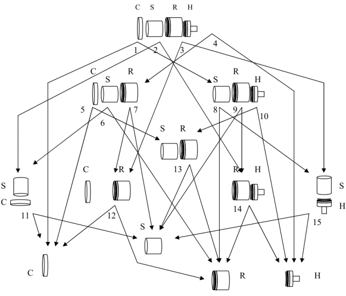
In AOG, each disassembly task is assumed to take apart the product or subassembly into exactly two new subassemblies. Two connected arcs that link the resulting two subassemblies of the disassembly task with the input node is called a hyper-arc (There are fifteen of them in Figure 6). There are nodes and hyper-arcs corresponding to the subassemblies and the disassembly tasks, respectively (Figure 6 is the AOG of the product in Figure 5). To see more about the concepts used here, you may refer to de Mello and Sanderson (1990, 1991 a, 1991b) or the Appendix 1 of this study.
Figure 5 A sample product (de Mello and Sanderson (1990))
cap stick receptacle handle
b) assembly in the disassembled form a) an assembly in a compact form
Figure 6 AND/OR Graph of the Product in Figure 5
To make a formal definition, let K be a set of elements and Π (K) be the set of all subsets of K. Consider a product A with parts PA = {p1, p2, …, pN}. There is
a unique AND/OR graph (AOG) of assembly/disassembly sequences for A defined as <SA, DA> such that; S = {θ∈Π (P ) sa (θ) = “T” ∧ st (θ) = “T”} [1] S H C S R H C C C S S S S R R R R R R H H H C S 1 2 3 4 5 6 7 8 11 12 13 14 10 9 15
is the set of nodes (subassemblies) in AOG and
DA = {(θk, {θi, θj}) [θk, θi, θj ∈ SA]∧[τ(θi, θj) = θk]∧gf (τ)=“T”∧mf (τ) =“T”} [2]
is the set of hyper-arcs, where ∧ is the and operator. τ is the assembly task, sa and st are subassembly and stability predicates, gf and mf are geometrical and mechanical feasibility predicates (Appendix 1). We discuss some properties of AOG’s in Section A1.4 of Appendix 1.
3.1.2 Assembly/Disassembly Tree (AT/DT)
We only need a subset of the tasks in AOG to completely assemble/disassemble the product. The question is how to select these tasks so that, when applied one after another, they achieve this goal. In fact, due to the nature of AOG, the set of these tasks constitutes a tree.
In AOG, an hyper-arc is said to be adjacent from a node, if the subassembly associated with the node is the input subassembly of the disassembly task corresponding to the hyper-arc. Similarly, an hyper-arc is said to be adjacent to a node, if the subassembly associated with the node is the output subassembly of the disassembly task corresponding to the hyper-arc. Correspondingly, the node to which the hyper-arc is adjacent is called the output node, and the node from which the hyper-arc is adjacent is called the input node. Each hyper-arc is adjacent from one input node and adjacent to two output nodes. The node to which none of the hyper-arcs are adjacent is called the initial node, and the nodes from which none of the hyper-arcs are adjacent are called the terminal nodes.
We define an AND/OR path in the graph as a set of hyper-arcs with k (>0) elements and their corresponding input and output nodes such that there are no two hyper-arcs that are adjacent from the same node, and there is only one initial node in the path. An AND/OR path that has k = N-1 elements is called assembly/disassembly tree (AT/DT) of the product. Note that, a DT (AT) should have {p1, p2,…, pN} as its initial (terminal) node and {p1}, {p2},…, {pN} as its
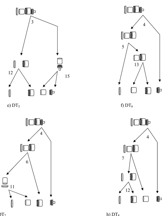
terminal (initial) nodes. Having N-1 hyper-arcs (assembly/disassembly tasks), a AT/DT represents one way of completely assembling/disassembling the product. In Figure 7, there are eight DT’s corresponding to the AOG in Figure 6
There are precedence relations among the hyper-arcs in the DT: Hyper-arc hi is said to immediately precede hyper-arc hj, if the output node of hi is the input
node of hj. Using these precedence relations between the hyper-arcs, we transform
the AT/DT’s to a new form called transformed AT/DT (TAT/TDT). Although TAT/TDT’s are like task precedence diagrams (TPD’s), we will not call them as TPD to differentiate each other. Figure 8 shows the 8 TDT’s corresponding to the 8 DT’s in Figure 7. In this study, for the sake of simplicity we will use the terms AT/DT instead of TAT/TDT.
In graph theory, a directed graph is said to be a tree if the corresponding undirected graph has no cycles. The number of directed arcs adjacent from a node is called the branch of the graph at the corresponding node. Based on this terminology, it is appreciated that AT/DT’s are trees with at most two branches. Expressing in the precedence-related words, in AT/DT, there is no task preceded by more than one task and there is no task preceding more than two tasks. Hence, AT/DT’s are restricted versions of TPD’s.
a) DT1 b) DT2 c) DT3 d) DT4 1 9 14 2 11 14 1 8 15 1 10 13
e) DT5 f) DT6
g) DT7 h) DT8
Figure 7 All of the 8 DT’s obtained from the AOG in Figure 2 4 6 11 4 7 12 3 12 15 4 5 13
a) Transformed disassembly tree 1 (TDT1) b) Transformed disassembly tree 2 (TDT2)
c) Transformed disassembly tree 3 (TDT3) d) Transformed disassembly tree 4 (TDT4)
e) Transformed disassembly tree 5 (TDT5) f) Transformed disassembly tree 6 (TDT6)
4 5 13 12 13 2 1 10 13 13 12 2 1 9 14 13 6 6 1 8 15 13 14 1 3 15 12 16 1 7 2 14 11 17 6 1
g) Transformed disassembly tree 7 (TDT7) h) Transformed disassembly tree 8 (TDT8)
Figure 8 Eight transformed disassembly trees (TDT) associated with the eight DT’s in Figure 4
3.2 Theorem of Sub-optimality
We extend the definition of classical ALB problem to cover disassembly studies as well. Since the disassembly is just the reverse of the assembly, from now on, we call ALB problem as assembly/disassembly line balancing (ADLB) problem. The ADLB problem for a task precedence diagram (TPD) has a fifty years’ of history. There are numerous approaches, both exact and heuristic (Erel and Sarin 1998, Baybars 1986). In this chapter, we define ADLB problem for an AOG and compare it with the ADLB problem for a TPD. To be concise, let ADLB-AOG show the latter problem and ADLB-TPD denote the former.
Definition 1 (ADLB-AOG problem): Choose a set of tasks from AOG such that the chosen set of tasks constitutes an AT, and the solution (number of stations) to the TPD problem for the chosen AT is the best (minimum) of the ADLB-TPD problems over all possible AT’s in AOG.
4 7 0 12 12 16 7 4 6 11 12 15 1
Both AOG and TPD include the precedence relations between the tasks to be applied to a product in the assembly/disassembly process. The tasks in AOG are defined based on two properties (Appendix A.1.2): (i) The subassembly it is applied to, (ii) and the contacts of the product it disassembles. The first property in the definition causes a set of tasks that disestablishes the same contacts to be labeled differently. For instance in Figure 10, tasks τ1 and τ5 break the same
contacts (c1, c2), i.e., disassembles {cap} from {receptacle}, but are labeled as
different tasks. Due to the first property, we call the tasks in AOG as subassembly-dependent tasks (SD tasks). On the other hand, the tasks in TPD are defined based only on the second property above. As a result, the tasks that break the same contacts are labeled as the same task independent of the subassembly they are applied to. Hence, we call the tasks in TPD as subassembly-independent tasks (SI tasks).
Theorem 1 (Theorem of sub-optimality):
The optimal solution to the ADLB problem for a given TPD of a product (XTPD* ) constitutes an upper bound on the optimal solution to the ADLB problem for the AOG (X*AOG) of the same product.
Proof: The solution to ADLB-TPD problem is a sequencing problem (Held and Karp, 1962). That is, each SI task sequence obtained from the TPD has its corresponding solution and one of these sequences characterizes the optimal solution. Based on this, we prove the theorem in two steps:
i) Any SI task sequence obtained from the TPD of a product is also obtainable from the AOG of the same product.
ii) The solution to an SI task sequence is an upper bound on the solution to the corresponding SD task sequence.
i) Each AT in AOG of a product includes a number of SD task sequences. Denote the set of AT’s as SAT. Re-label the tasks in each AT such that
the tasks that break the same contacts are labeled as the same tasks. Denote the resulting trees as ATm and the set of ATm’s asSATm. Note that AT
m
’s include SI task sequences. We should show that any sequence of SI tasks in a TPD is obtainable from one of the ATm’s in SATm .
Let a sequence of SI tasks beτSI1,τSI2,...,τSIn−1, where n is the number of parts in the product. Although these tasks are subassembly independent by definition, they are actually performed on specific subassemblies. With the additional consideration of subassemblies these tasks are defined in relation to subassemblies, and are called SD tasks. Let the corresponding sequence of SD tasks beτSD1,τSD2,...,τSDn−1. Since all possible ways to assemble/disassemble a product is embedded in AOG, the sequence τSD1,τSD2,...,τSDn−1is obtainable from one of the AT’s in SAT. Hence, the sequence τSI1,τSI2,...,τSIn−1 is inSATm .
ii) Let X*ATm be the best solution of the ADLB-TPD problem
onSATm and
* AT
X be the best solution onSAT. The argument in the second step holds if and only if X*ATm ≥
* AT
If the duration of the SD tasks and corresponding SI tasks had been the same, the two solutions, X*ATm and
* AT
X , would be the same. The re-labeling step in the procedure does not only re-label the SD tasks but also changes the durations of the tasks. When one or more SD tasks are re-labeled to form a single SI task, the duration of the resulting SI task should be taken as the maximum of durations of these SD tasks. Otherwise, the cycle time constraint would be violated. To be more specific, (w.l.o.g) suppose that;
τ11, τ12, …, τ1k is the only re-labeled SD tasks in AT1, AT2, …, ATk,
τ1 is the corresponding SI task in AT1m, AT2m, …, ATkm,
the duration of τ11 (dτ11) is the maximum of dτ11, dτ12, …, dτ1k
1
AT
X is not the best solution among XAT1, XAT2, …, XATk
Suppose that the duration of SI task τ1 (dτ1) is not set to the maximum
duration (dτ11). Then, m
AT
X
1 will be infeasible since the duration of τ1 in AT1
m
is considered to be smaller than the original duration, which is the duration of τ11 in
AT1. Hence, the job may not be completed within the cycle time. On the other
hand, if the duration of the SI task is set to the maximum of the durations of all corresponding SD tasks, there will be no violation of exceeding the cycle time.
Suppose that the duration of the SI task is set to the maximum of the durations of all corresponding SD tasks. The duration of τ1 in AT1m will be same
with the original duration, which is the duration of τ11 in AT1. Hence,
m
AT
X
1 = AT1
X . [3]
m AT X 2 ≥ AT2 X , m AT X 3 ≥ AT3 X m k AT X ≥ XATk [4] by [3] and [4], * * * * * * * * } ,..., , min{ } ,..., , min{ 1 2 2 1 AT AT AT AT AT AT AT AT X X X X X X X X k m k m m m = ≥ =
Figure 9 depicts theorem of sub-optimality.
Figure 9 Theorem of sub-optimality
PRODUCT STRUCTURE (AOG) SAT Solution XTPD* Solution XAOG* * TPD X
≥
≥
≥
≥
XAOG* Combination Re-labeling IP/D P ALB Algorithm m AT S STPD SAT Establishment3.3 The derivation of a TPD from the AOG
The ATm’s have the precedence relations between the SI tasks. In this respect, although it seems that each of them corresponds to a TPD of the product, they are still restricted version of a TPD, i.e., some of the ATm’s include exactly the same tasks and may be combined to form a TPD. Two ATm’s that have exactly the same tasks are called equitask ATm’s. To form a TPD from m
AT
S , one establishes the groups of equitask ATm’s and combines them to get one TPD for each group (Let the set of TPD’s be STPD). For instance, suppose that AT1m and
AT2m consist of two tasks τ1 and τ2. Also, τ1 is the predecessor of τ2 in AT1m and
successor of τ2 in AT2m. Then, AT1m and AT2m are equitask ATm’s. We combine
AT1m and AT2m so that the resulting TPD does not have precedence relation
between τ1 and τ2. Note that if there are no equitask ATm’s, each ATm corresponds
to a TPD.
In all of the ALB studies so far, researchers used TPD’s that only have AND-type precedence relations. In AND-type precedence relations, to accomplish a task one should perform all of its predecessors. On the other hand, to accomplish a task it may suffice to accomplish only one of its predecessors. We call these types of precedence relations OR-type. Inclusion of OR-type precedence relations in the TPD is more realistic. But in this study, while combining the ATm’s we only look for the AND-precedence relations between the tasks. The inclusion of OR-type precedence relations in establishing STPD from m
AT
S deserves a different study.
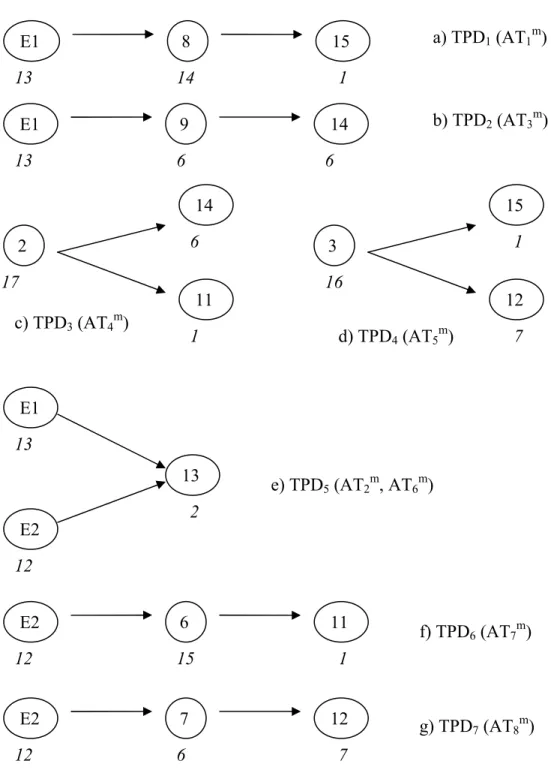
We give three examples for the derivation of TPD from the AOG.
Example 1
We consider the product in Figure 5. AOG of the product is in Figure 6. We obtain the set of AT’s (SAT) from the AOG in Figure 8. To re-label the SD
tasks as SI tasks we need to know which contacts each of the SD task break. In Figure 10, each SD task is demonstrated by the corresponding contacts and the subassemblies they are applied. It is seen that tasks τ1 and τ5 disestablish the same
contacts. Hence, they are re-labeled as E1. Also, the tasks τ4 and τ10 are re-labeled
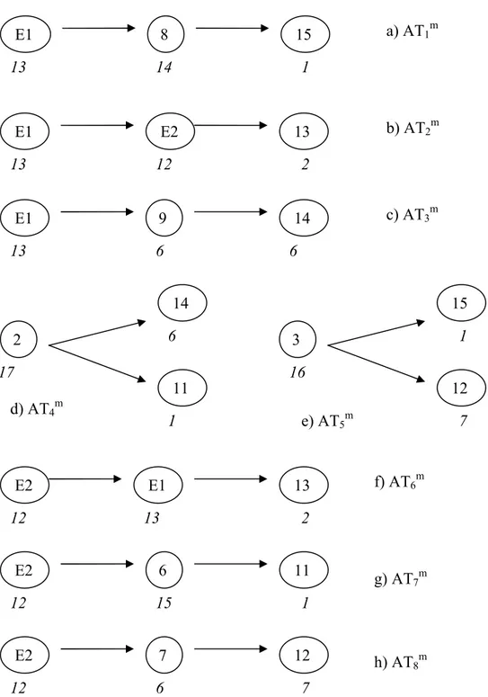
as E2. After re-labeling the tasks the AT’s become ATm’s. The resulting set of ATm’s (SATm ) is in Figure 11. We group the AT
m
’s that include exactly the same tasks (equitask ATm’s). There is only one group that includes more than one equitask ATm, which are AT2m and AT6m. Hence, all of ATm’s except the second
and the sixth are accepted as a TPD. AT2m and AT6m are combined to get TPD5.
c1 C R H S c2 c3 c5 c4 τ1 → c1, c2 = 13 τ2 → c2, c3, c4 = 17 τ3 → c1, c3, c5 = 16 τ4 → c4, c5 = 12 C R S c1 c2 c3 τ5 → c1, c2 = 11 τ6 → c2, c3 = 15 τ7 → c1, c3 = 6 C R H S c3 c5 c4 τ8 → c3, c5 = 14 τ9 → c3, c4 = 6 τ10 → c4, c5 = 10 C S c1 τ11 → c1 = 1 R c5 H τ14 → c5 = 6
Figure 10 The subassemblies of AOG in Figure 6, their GOC and corresponding tasks C R c2 τ12 → c2 = 7 R S c3 H S c4 τ13 → c3 = 2 τ15 → c4 = 1
a) subassembly b) GOC c) tasks with their durations and
Figure 11 The SATm obtained from SAT in Figure 8 E1 8 15 E1 E2 13 E1 9 14 2 14 11 3 15 12 E2 E1 13 E2 6 11 E2 7 12 a) AT1m b) AT2m c) AT3m d) AT4m e) AT5m f) AT6m g) AT7m h) AT8m 13 14 1 13 12 2 13 6 6 12 13 2 12 15 1 12 6 7 17 6 1 16 1 7
Figure 12 STPD obtained by combining equitask ATm’s in Figure 11 E1 8 15 E1 9 14 2 14 11 3 15 12 E2 6 11 E2 7 12 a) TPD1 (AT1m) b) TPD2 (AT3m) c) TPD3 (AT4m) d) TPD4 (AT5m) f) TPD6 (AT7m) g) TPD7 (AT8m) 13 14 1 13 6 6 12 15 1 12 6 7 17 6 1 16 1 7 13 E1 E2 13 2 12 e) TPD5 (AT2m, AT6m)
Example 2
All the related figures of this example are in Appendix 2. We consider the product in Figure A.7. We derive the AOG of the product (Figure A.8). Figure A.9 is the set of AT’s (SAT) obtained from the AOG. In Figure A.10, each SD task is
demonstrated by the corresponding contacts and the subassemblies they are applied to. By examining the contacts we re-label the tasks as below:
τj = τb = τs ⇒ τ1 (disassemble part 4)
τa = τc ⇒ τ2 (disassemble part 3 from part 9)
τk = τo ⇒ τ3 (disassemble part 2 from part 3)
τf = τh = τi ⇒ τ4 (disassemble part 7 from part 8)
τp = τd = τm ⇒ τ5 (disassemble part 9 from part 10)
τe = τg = τl = τq ⇒ τ6 (disassemble part 8 from part 9)
τn ⇒ τn (disassemble part 7 from parts 5 and 6)
τr ⇒ τr (disassemble part 5 from part 6)
τt ⇒ τt (disassemble part 1 from part 2)
The resulting SATm is in Figure A.11. We form the groups of equitask
ATm’s. There is only one group. That is, each of the ATm’s has includes the same tasks. Hence, we combine all ATm’s to get a single TPD, which is in Figure A.12.
Example 3
We consider the product in Figure A.13 of Appendix A3. AOG of the product is in Figure A.14. Figure A.15 is the set of AT’s (SAT). In Figure A.16,
each SD task is demonstrated by the corresponding contacts and the subassemblies they are applied to. By examining the contacts we re-label the tasks as below:
τ1 = τ6 = τ8 = τ14 = τ19 ⇒ τa τ2 = τ4 = τ10 = τ12 = τ18 ⇒ τb τ3 = τ5 = τ7 = τ11 ⇒ τc τ9 = τ15 = τ13 = τ17 ⇒ τd τ16 ⇒ τ16 τ20 ⇒ τ20 τ21 ⇒ τ21 τ22 ⇒ τ22 τ23 ⇒ τ23
The resulting SATm is in Figure A.17. We form the groups of equitask
ATm’s. There are two groups of equitask ATm’s. We combine AT2m, AT4m, AT5m,
AT7m, AT8m, AT10m, AT12m, AT13m, AT14m, AT15m, AT17m to get TPD1 and AT1m,
AT3m, AT6m, AT9m, AT11m, AT16m to get TPD2. The two TPD’s are in Figure A.18.
3.4 An Example to compare TPD and AOG.
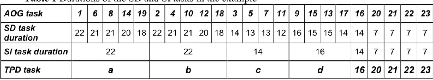
To illustrate the whole discussion in this chapter, we take the AOG and two resulting TPD’s in the Appendix 3. We assign the durations to the tasks of AOG as in the Table 1 below. Corresponding durations for the SI tasks of TPD1 and TPD2
Based on these durations, we solve ADLB-AOG and ADLB-TPD for two TPD’s. We solve the three problems for each value of cycle time (T) from 22 to 90. Since the task with the minimum duration has the duration of 22, cycle time can not have the value less then 22. We limit the cycle time with 90 because above 90 the results of ADLB-AOG and ADLB-TPD problems are the same. The solutions (number of stations) for each problem are listed in Table 2.
Table 1 Durations of the SD and SI tasks in the example
AOG task 1 6 8 14 19 2 4 10 12 18 3 5 7 11 9 15 13 17 16 20 21 22 23 SD task
duration 22 21 21 20 18 22 21 21 20 18 14 13 13 12 16 15 15 14 14 7 7 7 7
SI task duration 22 22 14 16 14 7 7 7 7
TPD task a b c d 16 20 21 22 23
In the Table 2, the leftmost column represents the problem when the cycle time is equal to that value. For instance, when the cycle time is 28 the ADLB-AOG problem yields a solution of 3 stations. On the other hand, the ADLB-TPD problem for TPD1 yields a solution of 5 and the problem for the TPD2 yields a
solution of 4. Hence, when the cycle time is 28, with all the other data being fixed as given, the ADLB-AOG problems yields better solutions than the ADLB-TPD problem no matter which TPD is used.
Table 2 The solutions to the three example problems
T AOG TPD1 TPD2 T AOG TPD1 TPD2 T AOG TPD1 TPD2
22 4 5 5 45 2 2 2 68 1 2 2 23 4 5 5 46 2 2 2 69 1 2 2 24 4 5 5 47 2 2 2 70 1 2 2 25 4 5 5 48 2 2 2 71 1 2 2 26 4 5 5 49 2 2 2 72 1 2 2 27 4 5 5 50 2 2 2 73 1 2 2 28 3 5 4 51 2 2 2 74 1 2 2 29 3 4 4 52 2 2 2 75 1 2 2 30 3 3 4 53 2 2 2 76 1 2 2 31 3 3 4 54 2 2 2 77 1 2 2 32 3 3 4 55 2 2 2 78 1 2 2 33 3 3 4 56 2 2 2 79 1 2 2 34 3 3 4 57 2 2 2 80 1 2 2 35 2 3 4 58 2 2 2 81 1 2 2 36 2 3 3 59 2 2 2 82 1 2 2 37 2 3 3 60 2 2 2 83 1 2 2 38 2 3 3 61 2 2 2 84 1 2 2 39 2 3 3 62 2 2 2 85 1 2 2 40 2 3 3 63 2 2 2 86 1 2 1 41 2 3 3 64 1 2 2 87 1 2 1 42 2 3 3 65 1 2 2 88 1 1 1 43 2 3 3 66 1 2 2 89 1 1 1 44 2 2 2 67 1 2 2 90 1 1 1
As can be easily seen from the table that if we pick up the TPD1 as the
precedence diagram and solve the ADLB-TPD problem for the cycle times 22-90, we obtain the actual optimal 28 times and fail at 41 of them. When we solve the ADLB-TPD problem for TPD2 we obtain the actual optimal 25 times and fail at 44
of them. To be on the optimistic side, if we take both of the TPD’s, solve ADLB-TPD problem for each of them and take the best solution, we get the actual
It is interesting that using even more than one TPD does not guarantee the optimal solution in ADLB-TPD problem. This is mainly due to the increase in durations of the SI tasks when they are re-labeled, as the theorem of sub-optimality suggests. When we think that researchers or practitioners consider only one TPD, the importance of ADLB-AOG problem stands out. What is more, although some TPD’s has OR-type precedence relations, in the literature TPD’s that are used has AND-type precedence relations. This deteriorates the solution of the ADLB-TPD problem further.
C h a p t e r 4
THE SOLUTON TO THE ADLB-AOG PROBLEM
In this chapter we construct an integer programming (IP) and dynamic programming (DP), to solve the ADLB-AOG problem. We also compare these two methods in terms of the size of the ADLB-AOG problem solved.
In the formulation process we do not use the AOG since it does not show explicitly the precedence relations between the tasks. Instead, we develop a new graph, called transformed AOG (TAOG). TAOG is formed as follows: Each node in the AOG corresponding to a subassembly is represented by an (artificial) node in TAOG. Each hyper-arc in the AOG associated with a task is represented by a (normal) node in TAOG. In TAOG, an artificial node is preceded by a normal node such that, in AOG, the hyper-arc associated with the node will be adjacent to the subassembly corresponding to the artificial node. Similarly, an artificial node precedes a normal node such that, in AOG, the hyper-arc associated with the node will be adjacent from the subassembly corresponding to the artificial node. We label the artificial nodes by Ai’s and normal nodes by Bi’s. In Figure 13 we give an
example TAOG of the AOG in Figure A.14 of Appendix 3. From now on, to make the notation more manageable, we use AOG to denote TAOG.
An artificial node may be preceded or succeeded by more than one normal node. But only one of the predecessors and one of the successors should be
processed. Hence, predecessors and successors of the artificial nodes are 1OR-type meaning that exactly one of them must be chosen and it does not matter which one it is. To differentiate between the AND-type and OR-type relations, we put a small curve as indicator of OR-type relations. The fact that there are OR-type relations in AOG reveals that only some percent of the tasks is sufficient to assemble/disassemble the product completely, as opposed to the TPD in which all the tasks should be accomplished. Appendix 4 shows how to store an AOG (TAOG) in a matrix.
Figure 13 Transformed AND/OR Graph of the AOG in Figure A.14 of Appendix 3
A13 B4 A4 B11 A0 B1 B2 B3 A1 A2 A3 B5 B6 B7 B8 B9 B10 A5 A6 A7 B12 B13 B14 B18 A8 A9 B15 A12 B16 B17 B19 A10 A11 B20 B21 B22 B23
4.1 The Proposed Dynamic Programming (DP) Formulation
The proposed DP approach solves the problem by finding the solutions to the partial problems, which eventually constitute the whole problem. It reduces the permutation-size solution space to combination-size (Held and Karp, 1962).
4.1.1 Definitions and Terminology 4.1.1.1 Partial AOG’s
In the formulation of the problem we use some new terminology. A partial AOG, AOG ({Ai}), is defined as a graph obtained from AOG in such a way that all
AT’s to be obtained from that partial graph should have Ai as one of their final
nodes. AOG ({Ai}) is obtained in two steps: First, delete nodes from AOG such
that the AT’s including the deleted nodes do not have the node Ai. Then, from the
resulting AOG, delete the node Ai together with all of its successors. We then
extend the definition of partial AOG to the following: Define AOG ({A1, A2, …, Ak}) to be the graph obtained in k steps: First, find AOG ({Ai1}) from AOG, then
find AOG ({Ai1, Ai2}) from AOG ({Ai1}), and so on until finding the AOG ({Ai1,
2
i
A , …, Aik−1, Aik}) from AOG ({Ai1, Ai2, …, Aik−1}). Note that the sequence of artificial nodes is arbitrary in this k-step procedure. By convention, AOG ({∅}) = AOG, and AOG ({A0}) = ∅. In Appendix 5, some examples to form partial AOG
are given.
Let S = {A1, A2, …, Ak} be a set of artificial nodes. Final nodes of an AOG
precede any other normal node in AOG (S). For instance the nodes B11, B12, B14
are the final nodes of the partial AOG in Figure A.21 of Appendix 5.
4.1.1.2 Assembly task sequences
We define assembly task sequences σ = (B1, B2, …, Bt) obtained from the
normal nodes (tasks) of AOG to be feasible if; i. P(Bi) ≠ P(Bj) ∀i ≠ j
ii. |{ B1, B2, …, Bi-1 } ∩ P(P(Bi))| = 1 ∀ i = 2, 3, …, t
where P(Bi) is the artificial predecessor of the normal node Bi, P(P(Bi)) is the
normal predecessor of the artificial node P(Bi) and | | is the cardinality operator
defined on the sets.
The first property above prevents the sequence from having the two OR-successors of an artificial node simultaneously. For instance the sequence {B1, B4,
B5} is prohibited by this property. Without the second property, the two normal
nodes that are not OR-successors of the same artificial node but belong to the different AT’s may exist in the sequence. For instance, the sequence {B1, B4, B11,
B13} is not allowed. Furthermore, the second property guarantees the normal nodes
to follow the precedence relations dictated by the AT they belong to. For example, the second property does not allow the sequence {B4, B11, B16, B20, B1, B21} since
the nodes (tasks) are not in the correct order, although they belong to the same AT. Final nodes of a sequence, denoted by F(σ), are defined to be nodes of the sequence such that the sequence still remains feasible when they are removed from the sequence. For instance the tasks B20 and B21 are the final nodes of the sequence
Associated with each feasible sequence σ is a particular assignment of tasks, represented by normal nodes, to the stations, called the induced assignment for σ. This assignment is obtained as follows: Assign as many tasks as possible from the beginning of the sequence to the first station, as many as possible from the beginning of the remaining subsequence to the second station, and so on, while not violating the cycle time (T) constraint. Intuitively, the induced assignment for a sequence is the optimal assignment. If the induced assignment for σ requires r
stations and w(r) is the sum of durations of the tasks assigned to the last station, the quantity cσ =
T w
r-(r)
1+ is a measure of the ‘cost’ of executing σ.
If a feasible sequence σ* is formed by adjoining a task Bt+1 to the end of σ,
then cσ* = cσ + Γ (cσ, dBt+1), where,
+ = + = + + < + < + − + = Γ T y x T y x or x T y x if T y T y x T y x x if T y x T y x y x / / / / / / / / ) , ([5]
where
x denotes the highest integer smaller than or equal to x.The above equation can be interpreted as follows; if the unused idle time in the last station that is used by the induced assignment σ is greater than or equal to
1 + t
B
d , then Γ = dBt+1/ T; otherwise, new station is opened, which causes to the term
related with the unused idle time to be added to
1 + t
B
4.1.1.3 Relation between partial AOG’s and assembly task sequences
There is a natural correspondence between partial AOG’s and feasible sequences defined by two mappings; G(σ) = { AOG(S) | F(σ) = F (AOG(S))},
G-1(AOG(S)) = {σ | G (σ) = AOG(S)}. Note that G is a one-to-many mapping. That is, for an AOG (S) the number of feasible sequences is greater than or equal to one, while for each feasible sequence there is only one AOG(S).
We define the cost of each partial AOG (S) as the cost of the sequence that has the minimum cost over all the sequences to be obtained from that partial graph. Hence, C (AOG (S)) = σ σ c S AOG G
min
−1( ( )) ∈4.1.2 The Proposed DP Approach
From the discussion it follows that, solving the ADLB-AOG problem is equivalent to find the quantity C (AOG (∅)). Furthermore, the minimum number of stations required for the assembly line to perform the complete assembly/disassembly of the product is
C(AOG(∅)
, where
x denotes the smallest integer greater than or equal to x.Before the formal setting, one can see how the DP method works. In the solution of the problem (i.e., the induced assignment), one of the final nodes of the AOG (∅) will be the last task. This task is chosen among the final nodes of the
sequences in which the last task is the chosen node. When the last node is chosen, say Bi, a graph that gives the rest of the solution is needed. This graph should be such that any task to be obtained from it should belong to the same AT of the AOG(∅) with the previously chosen task. This graph is AOG(∅∪P(Bi)). Proceeding in this manner until obtaining the AOG{A0} gives the desired result.
It follows from the terms AOG (S), F (AOG) and the equation [5] that C (AOG(S)) can be calculated by the following recursion:
C (AOG (S)) = ≠ ∪ Γ + ∪ = ∈ } {A S for )} ))), ( ( ( ( ))) ( ( ( { } {A S for 0 0 )) ( ( 0
min
i i B i i S AOG F B d B P S AOG C B P S AOG C [6]To see how the recurrence relations in [6] hold, it must be realized that, if the solution to ADLB-AOG problem for an AOG(S) yields a sequence of t tasks, the solution for the AOG(S ∪ P (Bi)) yields a sequence of t-1 tasks, where Bi ∈ F(AOG (S)). That is, the kth stage of the formulation is the set of AOG(S) that are solved to the sequences with (n-1-k) tasks, where n is the number of parts in the product. Hence, there are a total of n stages, together with stage 0, in the solution of the whole problem. Stage 0 has only one state, which is AOG (∅). Similarly, the final stage (stage n-1) has only one state, which is AOG ({A0}). The number of states in the other stages depends on both the number of parts in the product and the geometry of the parts (Appendix 1 A1.4).
The recurrence relations in [6] enable us to determine C (AOG (∅)) by a computation involving only partial AOG’s, which are much less than the number of feasible sequences. When the cost of AOG (∅) is found, the optimal sequence of the tasks can be obtained recursively by the equation below, finding Bt, then B t-1, and so on to B1: ) ))), ( (( ( ))) ( ( ( )) (
(AOG S C AOG S P Bi CAOG S P Bi dBi
C = ∪ +Γ ∪ )) ( (AOG S F B where i∈ [7]
The proposed DP is implemented in Java. We give the code In Appendix 6.
4.1.3 Example
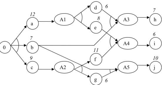
To illustrate the methodology explained in this section we solve an example problem for the AOG given in Figure 14. The durations of the tasks are given above the normal nodes. The cycle time (T) is 13.
There are three final nodes of AOG (∅∅∅∅), which are h, i, j. The partial AOG’s corresponding to them are AOG ({A3}), AOG ({A4}) and AOG ({A5}), respectively (Figure 15 –a, –b, –c). This gives the construction of stage 1 in Figure 16.
From [6], C (AOG (∅∅∅)) = min {C (AOG ({A∅ 3})) + Γ (C (AOG ({A3})), dh), C (AOG ({A4})) + Γ (C (AOG ({A4})), di),
Figure 14 TAOG of the AOG in Figure A.4 of Appendix 1
There are two final nodes of AOG ({A3}), which are d, j. The partial AOG’s corresponding to them are AOG ({A1}) and AOG ({A3, A5}), respectively (Figure 15 –d, –e). This is part of the construction of stage 2 in Figure 16.
From [6], C (AOG ({A3})) = min {C (AOG ({A1})) + Γ (C (AOG ({A1})), dd), C (AOG ({A3, A5})) + Γ (C (AOG ({A3, A5})), dj)} [9]
There are two final nodes of AOG ({A4}), which are e, f. The partial AOG’s corresponding to them are AOG ({A1}) and AOG ({A2}), respectively (Figure 15 –e, –f). This is part of the construction of stage 2 in Figure 16.
From [6], C (AOG ({A4})) = min {C (AOG ({A1})) + Γ (C (AOG ({A1})), de),
C (AOG ({A2})) + Γ (C (AOG ({A2 })), df)} [10] 0 c b a e d A1 A4 A2 g f A3 A5 j i h 12 7 9 6 8 11 7 6 10 6
There are two final nodes of AOG ({A5}), which are g, h. The partial AOG’s corresponding to them are AOG ({A2}) and AOG ({A3, A5}), respectively (Figure 15 –d, –f). This is part of the construction of stage 2 in Figure 16.
From [6], C (AOG ({A5})) = min {C (AOG ({A2})) + Γ (C (AOG ({A2})), dg), C (AOG ({A3, A5})) + Γ (C (AOG ({A3, A5})), dh)} [11]
There is only one final node of AOG ({A1}), which is a. The partial AOG corresponding to it is AOG ({A0}). This is part of the construction of stage 3 in Figure 16.
From [7], C (AOG ({A1})) = C (AOG ({A0})) + Γ (C (AOG ({A0})), da) [12]
There is only one final node of AOG ({A3, A5}), which is b. The partial AOG corresponding to it is AOG ({A0}). This is part of the construction of stage 2 in Figure 16.
From [7], C (AOG ({A3, A5})) = C (AOG ({A0})) + Γ (C (AOG ({A0})), db) [13]
There is only one final node of AOG ({A2}), which is c. The partial AOG corresponding to it is AOG ({A0}). This is part of the construction of stage 2 in Figure 16.
From [7], C (AOG ({A2})) = C (AOG ({A0})) + Γ (C (AOG ({A0})), dc) [14]