A new PI and PID control design method for integrating systems with time delays: applications to AQM of TCP flows

(1)

A New PI and PID Control Design Method for Integrating Systems

with Time Delays

DEN˙IZ ¨USTEBAY Bilkent University

Dept. of Electrical & Electronics Eng. 06800 Ankara

TURKEY deniz@ee.bilkent.edu.tr

H˙ITAY ¨OZBAY Bilkent University

Dept. of Electrical & Electronics Eng. 06800 Ankara

TURKEY hitay@bilkent.edu.tr

NAZLI G ¨UNDES¸ Univ. of California, Davis Dept. of Electrical & Computer Eng.

95616 CA USA

angundes@ucdavis.edu Abstract: Allowable PI and PD controller gains for a class of unstable MIMO systems with input/output delays have been investigated in [5, 12]. Using the results of these studies, we propose a new method for tuning the parameters of PI and PID controllers for integrating processes with time delays. As an application of this method, we design PI and PID controllers for Active Queue Management of TCP flows and illustrate performance of these controllers by packet level simulations in ns-2.

Key–Words: PID Controllers, Time Delay, Integrating Processes, Active Queue Management

1 Introduction

Proportional-Integral-Derivative (PID) controllers are widely used in various engineering applications since they are easy to implement using low storage mem-ory and their computational complexity is low, [1]. Many different types of tuning guidelines have been proposed in the literature, e.g. [1], [17], as design of PID controllers imply tuning of PID parameters. In this paper we consider integrating systems with time delays (i.e. the plant contains an integrator, a time de-lay, and possibly other stable terms). Tuning of PID controllers for this type of unstable time delay systems is an active research area, [8], [15], [17].

In a recent study, stabilizing PID controllers are obtained for a class of MIMO (input multi-output) unstable plants with delays in the input

and output channels, [12]. Using the results of

this study resilient PI (Proportional-Integral) and PD (ProportionDerivative) controllers with largest al-lowable controller gain intervals are investigated for plants with at most two unstable poles, [5]. In this paper, we use the results of these two studies to ob-tain the largest allowable gain intervals for a given set of nominal plant parameters and we propose to select the center of these intervals as the optimal gains of the controller. Controllers with perturbed gains can be seen as “optimal” controllers for plants with per-turbed nominal parameters. So, the controllers pro-posed here are expected to work for a wide range of plant parameters. Controllers using this method can be applied to integrating time delay systems appear-ing in data flow control in computer networks, target

tracking problems in robotics applications, and mate-rial transport systems encountered in process control. In this work, we consider the Active Queue Man-agement (AQM) of TCP flows as an application exam-ple. AQM tries to find a solution to congestion which is one of the most important problems in computer networks. When some of the links are congested, buffers at the routers are full, which means incom-ing packets are lost and re-transmission occurs. This leads to long return-trip-times (RTT), i.e. delays, and may even result in an instability in the network (e.g. congestion collapse in the Internet), [4]. On the other hand, having an empty queue at a buffer means that the link capacity is not fully used, i.e. network re-sources are under-utilized in this case. Therefore, the goal of AQM is to keep the queue size at the buffers at a certain desired level. For this purpose, most AQM schemes mark the Explicit Congestion Notification (ECN) bit of the packets passing through the link ac-cording to a certain rule. In early AQM methods, such as RED [3] and REM [2], packet marking probabil-ity (control signal) is a static function of the queue (or average queue). First attempts to design a dynamic controller appear in [6, 7], where the authors use the fluid model of the TCP flows developed in [10] to de-sign a PI controller. This AQM scheme is currently implemented in ns-2, [11]. It will be taken as the “benchmark” design for comparisons with the alter-native AQM controller tuning method proposed here.

Remaining of the paper is organized as follows. Details of the controller parameter tuning is given in Section 2. Application of this tuning method to the

(2)

AQM problem and comparisons with the benchmark PI design can be found in Section 3. Concluding re-marks are made in Section 4.

2 PI/PID Control for Integrating

Processes with Time Delay

One of the most attractive features of PID

(Proportional-Integral-Derivative) controllers is

their simplicity: in the most general form they are second order systems

Kpid(s) = Kp+K_si + Kds (1)

and can be implemented digitally by discretization. The main issue in PID control design is the “optimal” tuning of the gains, K_p, K_i, K_d.

Allowable ranges of PI and PD controller gains has been investigated in [5, 12]. Here we use these results to derive a controller for a plant whose transfer

function Gpq(s) is in the form

Gpq(s) = K_so e−hsg(s), h > 0 (2)

where g(s) is an arbitrary stable rational transfer func-tion satisfying g(0) = 1. For notafunc-tional convenience

we define f (s) := e−hsg(s) and let G(s) = Ko

s g(s)

be the finite dimensional part of the plant. A co-prime factorization of G(s) is in the form G(s) =

X(s)Y (s)−1 with X(0) = sG(s) |s=06= 0. In our

case, Y (s) = s/(as + 1), for any a > 0, and since

g(0) = 1, we have X(0) = Ko. Then a PI controller

is in the form

Kpi(s) = αX(0)−1(1 +γ_s) (3)

for α²R and γ²R. The bound on the integral

ac-tion gain γ can be defined by 0 < γ < γmax,

where γ_max−1 = kαsf (1+ α sf )−1−1 s k∞with α satisfying 0 < α < kf (s)−1_s k−1 ∞. Let us define θ := kf (s)−1s k∞.

Then the lower bound for γ_max−1 can be found as

γ∗ = α(1 − αθ) ≤ γmax. (4)

With straightforward calculation it can be shown that

the optimal α maximizing γ_∗is α_∗= 1

2θ and the

max-imal γ∗ corresponding to this optimal α is γ∗,max =

α∗

2 .

Here we propose to choose controller’s

propor-tional gain as α∗and integral gain as γ∗,max₂ , which is

the center of the maximal interval. The resulting PI controller is in the form

Kpi(s) = _2θ1 _K1

o

(1 + 1

8θs). (5)

The computation of (5) above is rather simpli-fied thanks to conservatism introduced by (4). In fact,

γ−1 maxis a function of α: γ_max−1 = sup ω ¯ ¯ ¯ ¯_{jω + αf (jω)}1 ¯ ¯ ¯ ¯ =: Q(α). This norm should be calculated for every α in the

in-terval 0 < α < 1/θ. Then γ−1

max could be chosen as

the minimum of Q(α). However, this method requires M ∗ N calculations for M being the ω grid points for

H∞norm computation and N being the α grid points.

Using (4) we skip the H∞norm computation for

ev-ery fixed α. The conservatism introduced by (4) is currently under investigation.

For a PD controller written in the form bK(1 +

b

Kds), [12] determined the optimal bKd maximizing

the allowable interval for the overall controller gain b

K within the framework of the approach introduced in [5]. In this paper, we propose to take this opti-mal derivative action gain, and the center of the

max-imal allowable interval for bK, for the plant (2). For

this purpose, define ρ(ω) := |f (jω)| and φ(ω) := ∠f (jω) as the magnitude and phase functions. Then set η(ω) := ¯ ¯ ¯ρ(ω)−cos(φ(ω))_ω ¯ ¯

¯ . Assume that η(ω) has a

maximum, ηo, which is attained at a single frequency

ωo. Then, define bKd := −sin(φ(ω_ω_o _ρ(ωo_o))₎ . With the above

definitions, the PD controller is

Kpd(s) = _2K1

oηo (1 + bKds). (6)

The above PD controller design technique is valid for all plants in the form (2) where g(s) can be any stable rational transfer function satisfying g(0) = 0, with one caveat: one has to check that the corresponding η has a single maximum. For a first order strictly proper g(s) (as in the AQM problem, to be shown below) this is automatically satisfied.

A PID controller can be obtained from the prod-uct of PI and PD controllers. So, we will design a PD controller, then design a PI controller for the PD

con-trolled open loop plant Gpq(s)Kpd(s). For this

pur-pose we define Gpq(s)Kpd(s) ≈ K_so e−hsg(s)_2K1 oηo (1 + bKds) =: 1 2ηo e−hs_g o(s) s go(s) := g(s) (1 + bKds) θo := kgo(s) − 1_s k∞. Kpi(s) = _2θ1 o 2ηo(1 +_8θ1 os ).

(3)

So, the PID controller is K_pid(s) = (1 + bKds) 16K_oθ2 o (1 + 8θos) s . (7)

3 Application to AQM

3.1 Fluid Model of TCP Flows

For AQM design a PI tuning method is proposed in [6, 7] using a dynamical model of the TCP. This model is introduced in [10], and has been tested and used by many researchers, see e.g. [9], [13], [14], [16], [19], and references therein. By making fluid approxima-tions the model is expressed in continuous time do-main as follows, [6] ˙ W (t) = 1 R(t) − W (t) W (t − R(t)) 2 R(t − R(t)) p(t − R(t)) (8) ˙q(t) = N (t)W (t) R(t) − c(t) when q(t) > 0 (9)

where W is the TCP window size, q is the queue length, N is the number of TCP flows passing through the link, c is the link capacity (outgoing flow rate),

R(t) = To+q(t)_c(t) is the RTT (total delay in the

feed-back path), T_o is the propagation delay, and p is the

probability of a packet being marked. In this sys-tem p can be seen as the control input generated by a feedback from q, i.e. p = K(q) where K is the feedback control operator. First AQM schemes devel-oped, e.g. RED, use static maps from q to p. Dy-namic controllers are developed recently using con-trol theoretic design methods. Clearly, the above sys-tem is nonlinear and it depends on an implicit function R(t−R(t)). In general, “optimal” controllers for such nonlinear dynamical systems are difficult to obtain. Typically, linearization is done around an equilibrium.

Let q(t) = q_o+ δ_q(t), W (t) = W_o+ δ_W(t), c(t) =

co + δc(t), N (t) = No+ δN(t), p(t) = po + δp(t)

and R(t) = Ro+ δR(t), with Ro = To+ q_co_o, where

qo, Wo, co, No, po, Ro are the nominal values

deter-mined from equilibrium conditions. Then, a transfer

function, Gpq(s), from the control input δpto the

out-put to be regulated δqcan be obtained using small

sig-nal asig-nalysis, see e.g. [6, 7, 14],

Gpq(s) = RocoK (Ros +_K1) e−Ros (Ros + 1), K = Roco 2No. (10)

If we assume that K À 1, then the “plant” (10) is

approximately in the form (2) with K_o := c_oK, h =

Roand g(s) = (1 + Ros)−1. Hence, we can apply the

technique proposed in Section 2.

Note that for (10) we can design a PI controller and then the PI controlled system can be considered as an open loop plant with an integrator so that we can apply PD control. This will be an alternative method of obtaining a PID controller. For the plant (10) the transfer function of the PI controlled system can be written as Gpq(s)Kpi(s) = KR_16θ₂o (8θs + 1)e −Ros s(KRos + 1)(Ros + 1) =: KRo 16θ2 go(s) s

For designing a PD controller, first define ρν(ω) :=

|gν(jω)| and φν(ω) := ∠gν(jω) as the new

mag-nitude and phase functions. Then set ην(ω) :=

|ρν(ω)−cos(φν(ω))

ω |. Assume that ην(ω) has a

max-imum, ην,o, which is attained at a single

fre-quency ων,o. With this assumption define bKdν :=

−sin(φν(ων,o))

ων,oρν(ων,o). Then the PD controller is

Kν,pd(s) = _2η1

ν,o

16θ2

KRo(1 + bKdνs).

Thus the overall PID controller for the plant (10) is

the product of Kpi(s) and Kpd(s), that is,

Kpid(s) = _2η(1 + bKdνs) ν,ocoRoK2

(1 + 8θs)

s . (11)

3.2 Simulation results

The simulation topology is a dumbbell network with a single bottleneck link shared by N TCP connections which generate FTP flows as in [18]. This bottleneck

link is of capacity C0 = 10 Mbps with T0 = 20 ms

delay. The links between the TCP sources and the first router, and the links between the TCP sinks and

the second router are C1 = C2 = 10 Mbps links with

T1 = T2 = 40 ms propagation delay, see Figure 1.

The buffer sizes of both routers are set to 300 packets and each packet is of size 1000 Bytes.

. . . . . . Router 1 Router 2 C1 T1 C2 T2 1 2 1 2 N N C0 T0

Figure 1: Network Topology

The nominal system parameters are: No = 30

TCP flows, c = C₀ = 1250 packets/s, q_o= 150

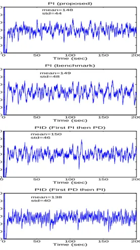
pack-ets, Ro = 0.32 s. The queue length plots of the

(4)

0 50 100 150 200 0 50 100 150 200 250 300 Time (sec)

Queue Length (packets)

PI (proposed) mean=148 std=44 0 50 100 150 200 0 50 100 150 200 250 300 Time (sec)

PI (benchmark) mean=149 std=48 0 50 100 150 200 0 50 100 150 200 250 300 Time (sec)

PID (First PI then PD)

mean=150 std=46 0 50 100 150 200 0 50 100 150 200 250 300 Time (sec)

PID (First PD then PI)

mean=138 std=40

Figure 2: ns-2 simulations: queue length vs time.

In order to evaluate these simulation results we first look at the RMS value of the percentage error of the queue length with respect to the desired queue

length, qd= 150 packets, more precisely,

RMS error = Ã 1 M M X k=1 µ q(k) − qd qd ¶₂!1 2 , (12)

here M is the total number of the samples generated by ns-2. Secondly, we specify a tolerance for tracking of the desired queue: let Q_d:= [q_d− q_tol, q_d+ q_tol] be a neighborhood of the desired queue. In our case we

have qd= 150 packets, and we choose qtol= 30

pack-ets. Define T0to be the total length of the time

inter-vals for which q(t) /∈ Qd, and let Ttotalbe the length

of the total simulation time (in our setting Ttotal= 200

seconds). Then the second error metric we are

inter-ested in is E = T0/Ttotal. This error provides a

bet-ter look on the variations of the queue length, and its small values bound the delay jitter.

Table 1 shows that the proposed PI controller per-forms better than the benchmark PI controller for both error metrics defined above. Note that all cost func-tions are normalized with respect to the time interval. The new proposed PI design gives an improvement of

Table 1: The analysis of simulation results

Controller RMS error E

PI (proposed) 0.29 0.28

PI (benchmark) 0.32 0.37

PID (first PI then PD) 0.30 0.30 PID (first PD then PI) 0.27 0.29

3% to 9% depending on the cost taken; when inte-grated over time, the benefits of the new design can be significant.

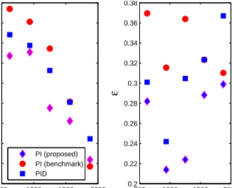
Furthermore, we investigate the robustness of the proposed controller schemes under variations of num-ber of TCP connections (load) N , the round trip time RT T and, the link capacity c. The controller designs are for the nominal values of the system parameters, as in the previous section, and are fixed throughout the robustness tests. The results of these tests are given in the Appendix. In Figures 3, 4 we vary the number of TCP connections from 10 to 60. In Figures 5, 6 the round trip time is varied between 160 msec and 480 msec. In Figures 7, 8 the capacity is changed from 625 packets/second to 1875 packets/second (from 5 Mbps to 15 Mbps). These figures illustrate the mean and standard deviations of the queue lengths and the error metric comparisons. We omitted the results for the second PID controller (first PD then PI), because it yields similar results to that of the first PID controller (first PI then PD).

As seen in all the figures related to performance robustness analysis, the proposed PI controller per-forms better than the PI benchmark design except for small values of N . The PI controller scheme that we propose here gives better results than PI benchmark for standard deviation and for both of the error met-rics. Simulation results showed that in certain situa-tions the proposed PI controller is better than the PID controller as far as the robustness is concerned.

4 Conclusions

In this paper we proposed new PI, PD and PID con-troller tuning methods for integrating systems with time delay using the analysis of allowable PID gains done in [5, 12]. The PI and PD controller expressions (5), (6) appearing in Section 2 are valid for all inte-grating systems whose transfer function is in the form (2) where g(s) is an arbitrary stable transfer function containing a time delay and satisfying g(0) = 0.

We have illustrated this method on the AQM problem for a single bottleneck network of TCP flows.

(5)

Performance of the proposed designs are compared with the benchmark design of [6, 7] implemented in ns-2. Simulations show that steady state queue vari-ations are lower in the new design, and the transient response performance is better. Robustness of the de-signs with respect to variation in R, N and c are also analyzed and we have seen that in almost all cases the new PI controller performs better than the benchmark PI controller.

References:

[1] K. J. Astr¨om, T. Hagglund, PID Controllers:

Theory, Design, and Tuning 2nd Ed., Instrument Society of America, Research Triangle Park, NC, 1995.

[2] S. Athuraliya, S. H. Low, V. H. Li, Q. Yin,

“REM: Active Queue Management,” IEEE Net-work, vol. 15 (2001), no. 3, pp. 48-53.

[3] S. Floyd, V. Jacobson, “Random early detection

gateways for congestion avoidance,” IEEE/ACM Transactions on Networking, vol. 1 (1993), no. 4, pp. 397-413.

[4] S. Floyd, K. Fall, “Promoting the use of

end-to-end congestion control in the Internet,” IEEE/ACM Transactions on Networking, vol. 7 (1999), pp. 458–472.

[5] A. N. Gündes¸, H. Özbay, A. B. Özgüler, “PID

Controller Synthesis for a Class of Unstable MIMO plants with I/O Delays,” Automatica, vol. 43 (2007), pp. 135–142.

[6] C. Hollot, V. Misra, D. Towsley, W. Gong, “On

designing improved controllers for AQM routers supporting TCP flows,” in IEEE INFOCOM, Alaska, April 2001, pp. 1726-1734.

[7] C. Hollot, V. Misra, D. Towsley, W. Gong,

“Analysis and design of controllers for AQM routers supporting TCP flows,” IEEE Transac-tions on Automatic Control, vol. 47 (2002), no. 6, pp. 945-959.

[8] Y. Lee, J. Lee, S. Park, “PID controller tuning

for integrating and unstable processes with time delay,” Chemical Engineering Science , vol. 55, 2000, pp. 3481-3493.

[9] S. Low, F. Paganini, J. Wang, S. Adhalka, J.

Doyle, “Dynamics of TCP/RED and a scalable control,” in Proc. IEEE INFOCOM, New York, June 2002, pp 239-248.

[10] V. Misra, W. Gong, D. Towsley, “A fluid-based

analysis of a network of AQM routers support-ing TCP flows with an application to RED,” in Proc. ACM SIGCOMM, Stockholm, Sweeden, Sep. 2000, pp. 151-160.

[11] ns-2 Network Simulator, version: 2.27. [Online].

Available: http://www.isi.edu/nsnam/ns/.

[12] H. ¨Ozbay, A. N. G¨undes¸, “Resilient PI and PD

Controllers for a Class of Unstable MIMO plants with I/O Delays,” Proc. of 6th IFAC Workshop on Time Delay Systems, L’Aquila, Italy, July 2006.

[13] E-C. Park, H. Lim, K-J. Park, C-H. Choi,

“Anal-ysis and design of the virtual rate control algo-rithm for stabilizing queues in TCP networks,” Computer Networks, vol. 44 (2004), pp. 17-41.

[14] P-F. Quet, H. ¨Ozbay, “On the Design of AQM

Supporting TCP Flows Using Robust Control Theory ,” IEEE Transactions on Automatic Con-trol, vol. 49 (2004), no. 6, pp. 1031-1036.

[15] E. Poulin, A. Pomerlau, “PI Settings for

Inte-grating Processes Based on Ultimate Cycle In-formation” IEEE Transactions on Control Sys-tems Technology, vol. 7, 1999, pp. 509-511.

[16] S. Ryu, C. Rump, C. Qiao, “A predictive and

ro-bust active queue management for Internet con-gestion control,”in Proc. of the 8th IEEE Sympo-sium on Computers and Communications, Ke-mer, Antalya, Turkey, June-July 2003, pp. 991– 998.

[17] G. J. Silva, A. Datta, S. P. Bhattacharyya, “PID

Controllers for Time-Delay Systems,” 2nd Ed., Birkh¨auser, Boston, 2005.

[18] P. Yan, Y. Gao, H. ¨Ozbay, “A Variable Structure

Control Approach to Active Queue Management for TCP with ECN,” IEEE Transactions on Con-trol Systems Technology, vol. 13 (2005), no. 2, pp. 203-215.

[19] P. Yan and H. ¨Ozbay, “Robust Controller Design

for AQM and H∞ Performance Analysis,” in

Advances in Communication Control Networks, S. Tarbouriech, C. Abdallah, J. Chiasson Eds., Springer-Verlag LNCIS, Vol. 308, 2004, pp. 49-64.

Acknowledgements: This work is supported by the European Commission (contract no. MIRG-CT-2004-006666) and by TUBITAK (grant no. EEEAG-105E156)

(6)

5 Appendix: Simulation Results

0 20 40 60 100 110 120 130 140 150 160 N

Mean value of queue length (packets)

0 20 40 60 35 40 45 50 55 60 65 N

Standard dev. of queue length (packets)

PI (proposed) PI (benchmark) PID

Figure 3: Mean and standard deviation of queue length under load variations

0 20 40 60 0.25 0.3 0.35 0.4 0.45 0.5 0.55 0.6 N RMS error 0 20 40 60 0.2 0.3 0.4 0.5 0.6 0.7 0.8 0.9 1 N ε PI (proposed) PI (benchmark) PID

Figure 4: Errors under load variations

0.1 0.2 0.3 0.4 0.5 138 140 142 144 146 148 150 152 154 156 RTT (sec)

0.1 0.2 0.3 0.4 0.5 30 35 40 45 50 55 60 RTT (sec)

Figure 5: Mean and standard deviation of queue length under RTT variations

0.1 0.2 0.3 0.4 0.5 0.2 0.22 0.24 0.26 0.28 0.3 0.32 0.34 0.36 0.38 0.4 RTT (sec) RMS error 0.1 0.2 0.3 0.4 0.1 0.15 0.2 0.25 0.3 0.35 0.4 0.45 0.5 RTT (sec) ε PI (proposed) PI (benchmark) PID

Figure 6: Errors under RTT variations

500 1000 1500 2000 140 142 144 146 148 150 152 154 Capacity (packets/sec)

500 1000 1500 2000 34 36 38 40 42 44 46 48 Capacity (packets/sec)

Figure 7: Mean and standard deviation of queue length under capacity variations

500 1000 1500 2000 0.23 0.24 0.25 0.26 0.27 0.28 0.29 0.3 0.31 0.32 Capacity (packets/sec) RMS error 500 1000 1500 2000 0.2 0.22 0.24 0.26 0.28 0.3 0.32 0.34 0.36 0.38 Capacity (packets/sec) ε PI (proposed) PI (benchmark) PID