The relationship between defense spending and inflation : an emprical analysis for Turkey

THE RELATIONSHIP BETWEEN DEFENSE SPENDING AND INFLATION: AN EMPRICAL ANALYSIS FOR TURKEY

The Institute of Economics and Social Sciences of

Bilkent University

by

TAYFUN GÜNANA

In Partial Fulfillment of the Requirements for the Degree of

MASTER OF BUSINESS ADMINISTRATION

in

THE DEPARTMENT OF MANAGEMENT BİLKENT UNIVERSITY

ANKARA July 2004

I certify that I have read this thesis and have found that it is fully adequate, in scope and in quality, as a thesis for the degree of Master of Business Administration.

--- Asst. Prof. Levent Akdeniz

I certify that I have read this thesis and have found that it is fully adequate, in scope and in quality, as a thesis for the degree of Master of Business Administration.

--- Asst. Prof. Aslıhan Altay Salih

I certify that I have read this thesis and have found that it is fully adequate, in

scope and in quality, as a thesis for the degree of Master of Business Administration.

--- Assoc. Prof. Faruk Selçuk

Approval of the Institute of Economics and Social Sciences

--- Prof. Dr. Kürşat Aydoğan

ABSTRACT

THE RELATIONSHIP BETWEEN DEFENSE SPENDING AND INFLATION: AN EMPRICAL ANALYSIS FOR TURKEY

Günana, Tayfun

M.B.A., Department of Management Supervisor: Asst. Prof. Levent Akdeniz

July 2004

This study estimates the relationship between defense expenditures and inflation

in Turkey over the period of 1950-2001 by employing a Johansen Cointegration analysis and Granger Causality test. The different views that appear in the literature on this relationship are identified and it is concluded that there is no

agreement as to the exact nature of the relationship between defense spending and inflation. The results of this study indicate that defense expenditures and inflation have a significant effect on each other both in the long and in the short

run. In other words, there is Granger feedback (X ↔ Y) between defense spending and inflation for Turkey.

Keywords: Defense expenditures, inflation, budget deficit, money growth,

ÖZET

SAVUNMA HARCAMALARI İLE ENFLASYON ARASINDAKI İLİŞKİ: TÜRKİYE İÇİN AMPRİK BİR ÇALIŞMA

Günana, Tayfun

Yüksek Lisans Tezi, İşletme Fakültesi Tez Yöneticisi: Yrd.Doç.Dr. Levent Akdeniz

Temmuz 2004

Bu çalışma, Johansen ko-entegresyon analizini ve Granger Nedensellik testini kullanarak, 1950-2001 yılları arasında Türkiye’de savunma harcamaları ile enflayon arasindaki ilişkiyi ortaya koymaya çalışmaktadır. Tez içerisinde bu

konu ile ilgili literatürde yer alan değişik görüşler ortaya konmuş ve savunma harcamaları ile enflasyon arasındaki ilişkinin yönü ve yapısı hakkında bir fikir birliğine varılamadığı görülmüştür. Yapılan çalışmanın neticesinde, savunma harcamaları ile enflasyonun birbirleri üzerinde hem uzun dönemde, hem de kısa

dönemde önemli etkilerinin olduğu görülmüştür. Başka bir deyişle, Türkiye’de, savunma harcamaları ile enflasyon arasında bir Granger geri besleme süreci mevcuttur.

Anahtar Kelimeler: Savunma harcamaları, enflasyon, bütçe açığı, para arzı

ACKNOWLEDGMENTS

I am very grateful to Asst. Prof. Levent Akdeniz for his supervision, constructive comments, and patience throughout the preparation of this thesis. I also wish to

express my thanks to Assoc. Prof. Selami Sezgin for his contributions in the data gathering for defense expenditures. Finally, I am grateful to my wife Gülseren, my daughter Dilan, and parents, to whom this thesis is dedicated, for their support, encouragement and patience.

TABLE OF CONTENTS

CHAPTER 2: BUDGET DEFICIT, MONEY GROWTH AND INFLATION.………..……….. ………..…. 10

2.1 Theoretical Background………...…..………....…..10

2.2 Brief Literature Survey on Recent Economic Studies...…….…...15

CHAPTER 3: LITERATURE REVIEW………...……….19

3.1 Different Views on Defense Spending-Inflation Relationship..…...19

3.1.1 Defense Spending Affects Inflation………...…..19

3.1.2 Inflation Affects Defense Spending………...……..27

3.1.3 Two-way Relationship between Defense Spending and Inflation ………...………..………..…28

3.1.4 No Relation between Defense Spending and Inflation...…...28

4.1 Data………...33

4.2 Unit Root Tests………...………..34

4.3 Johansen’s Cointegration Estimation Method……….……..38

4.4 Granger Causality Test………..42

CHAPTER 5: RESULTS……….………46

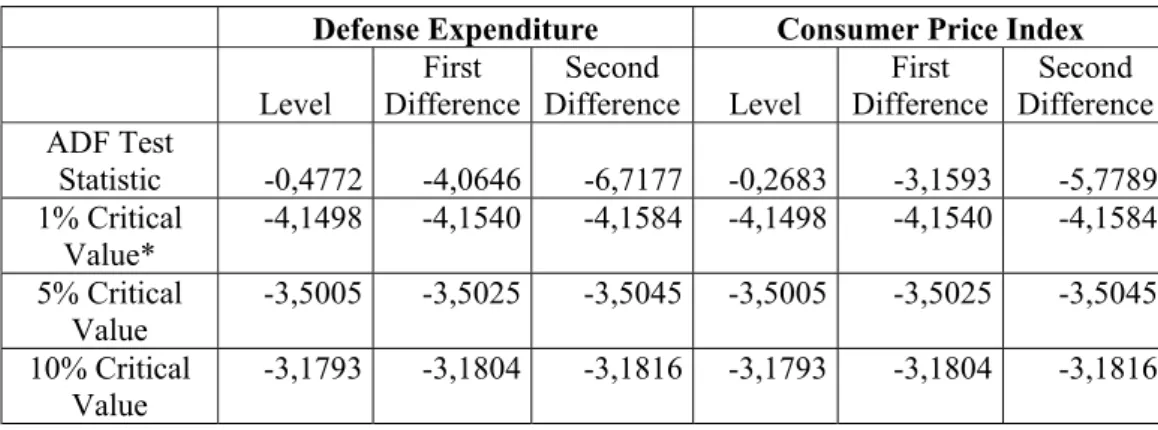
5.1 Unit Root Test………...46

5.2 Cointegration Test……….49

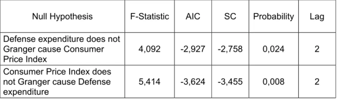
5.3 Causality Test………52

CHAPTER 6: CONCLUSIONS………...56

BIBLIOGRAPHY……….………58

APPENDIX A:Major Spenders in 2003………..64

LIST OF TABLES

Table 1 Military Expenditure by Region, in Constant US dollars, 1992-2001……….….……..2

Table 2 Military Expenditures of Turkey and Its Neighbors……….3

Table 3 Unit Root Test Results………..……….…….46

Table 4 Johansen Cointegration Test Results in Terms of Maximum

Eigenvalue Statistic ………..……….…….50

Table 5 Johansen Cointegration Test Results in Terms of Trace

Statistic……….…….…………..51

Table 6 Standardized Eigenvectors and Adjustment Coefficients …...……51

LIST OF FIGURES

Figure 1 Defense Expenditures as a Share of General Budget……….6

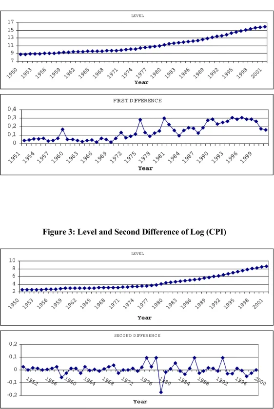
Figure 2 Level and First Difference of Log (defense expenditure)………..47

Figure 3 Level and Second Difference of Log (CPI)……….………..47

CHAPTER 1

INTRODUCTION

Initially, it is important to know the reasons why Turkey gives great importance

to defense. The threats and risks that Turkey has confronted with in the post-Cold War period are rather different from those in the past. At the end of the Cold War and the struggle between blocks, there was a search for a new world order by the effect of globalization, which also changed the concepts of threat.

While the concept of threat was previously evident and large at the beginning of the twenty-first century, it has become multi-directional, multi-dimensional. The traditional concept of threat has now started to contain new threats and risks emerging in the form of (White Book, 2002, Part IV):

– Regional and ethnic conflicts,

– Political and economic instabilities and uncertainties in the countries, – Proliferation of weapons of mass destruction and long-range missiles,

– Religious fundamentalism,

– Smuggling of drugs and all kinds of weapons and – International terrorism.

As one of the main centers of attraction due to its historical heritage, cultural

richness, democracy, economy and modernity, Turkey is located in the midst of regions such as the Middle East, the Caucasus and the Balkans, where the balances are undergoing a process of change and which are full of instability and uncertainty. It is obvious in Table 1 that the strongest growth in military

expenditure is realized in Middle East in which Turkey is located. As a result of extreme nationalist, expansionist and aggressive tendencies of its regional neighbors, Turkey lives together with the threats of radical fundamentalist movements, the proliferation of weapons of mass destruction, long-range

missiles, and terrorism, in particular.

Table 1: Military Expenditure by Region, in Constant US dollars, 1992-2001

1992 1993 1994 1995 1996 1997 1998 1999 2000 2001 World Total 847 814 793 741 722 732 719 728 757 772 Africa 9,3 8,8 9,3 8,9 8,5 8,8 9,3 10,9 11,3 12,2 Americas 383 367 348 333 314 315 308 308 319 317 Asia and Oceania 105 108 109 112 115 117 117 119 123 129 Europe 296 278 275 239 235 238 227 233 241 242 Middle East 52,3 51 50,9 47,9 48,9 53,5 57,8 56,1 63,1 72,4 NATO 557 533 508 481 466 462 457 467 478 472

Note: (1) Figures are in US $b., at constant 1998 prices and exchange rates. (2) Source: SIPRI Yearbook, 2002.

The primary and most important defender of Turkey’s independence is the Armed Forces. In today’s Turkey, the primary missions of the Turkish Armed

Forces are the defense and protection of the nation and the Republic, and the

fulfillment of the NATO duties assigned by international treaties. The Turkish Armed Forces aim to modernize and upgrade their weapons systems to bring them into line with NATO standards, the better to defend national independence

and to fulfill the requirements of a collective defense system.

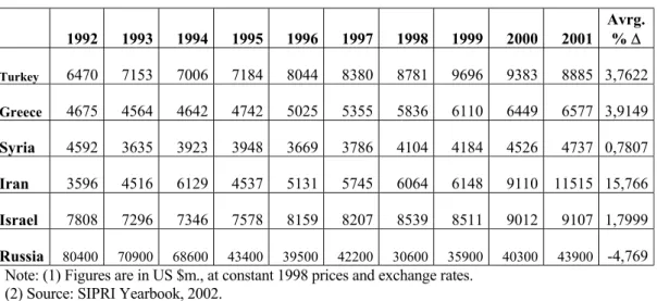
With the end of Cold War and East-West armaments race, military expenditures

have shown a decreasing trend across many countries. However, Turkey and its neighbors are exceptions to the worldwide decreasing military trend for different as well as interrelated reasons (See Table 2).

Table 2: Military Expenditures of Turkey and Its Neighbors

1992 1993 1994 1995 1996 1997 1998 1999 2000 2001 Avrg. % ∆ Turkey 6470 7153 7006 7184 8044 8380 8781 9696 9383 8885 3,7622 Greece 4675 4564 4642 4742 5025 5355 5836 6110 6449 6577 3,9149 Syria 4592 3635 3923 3948 3669 3786 4104 4184 4526 4737 0,7807 Iran 3596 4516 6129 4537 5131 5745 6064 6148 9110 11515 15,766 Israel 7808 7296 7346 7578 8159 8207 8539 8511 9012 9107 1,7999 Russia 80400 70900 68600 43400 39500 42200 30600 35900 40300 43900 -4,769 Note: (1) Figures are in US $m., at constant 1998 prices and exchange rates.

(2) Source: SIPRI Yearbook, 2002.

Given the fact that Turkey is subject to multi-dimensional internal and external threats due to its geopolitical and geostrategic location, the achievement of a military strength capable of supporting national security policy, the maintenance

requirements of the century, serve as the milestones of the policy and strategy of

Turkey. Being a strength and balance element in the region, Turkey pays more attention to defense than some other countries. With the purpose of maintaining her national existence, of strengthening her defenses and keeping pace with technological progress, Turkey allocates adequate funds to national defense

within existing possibilities. Turkey ranked first in arms imports among NATO members and second in the Middle East during 1992-1996. Turkey’s share in NATO imports increased from 20% in 1987 to 36% in 1996. According to SIPRI (Stockholm International Peace Research Institute) data, despite the fact

that military expenditures of the European NATO declined on average by 1% during 1985-1996, Turkey increased its military expenditures on average by 4%. In addition, Turkey has the fourteenth largest defense spending throughout the

world (See Appendix A).

It will be useful at this point to give the definition of military expenditure in order to make reliable comments on this topic. SIPRI, whose data are used in this

study, gives the definition of military expenditure that is based on NATO definition:

SIPRI military expenditure data include all current and capital expenditure on: (a) the armed forces, including peacekeeping forces; (b) defense ministries and other government agencies engaged in defense projects; (c) paramilitary forces, when judged to be trained and equipped for military operations; and (d) military space activities.

Defense is not a free good; like all expenditures, it involves sacrifices of other

goods and services, raising controversies about military versus social-welfare spending and whether defense is a benefit or burden to an economy. Such issues arise in both rich and poor countries. The economic implications of increased expenditures on arming, especially since 1980, have been an interesting issue for

scholars in Turkey. Although a number of studies concerning Turkish defense-growth relation have been published in recent years, little attention is given the relationship between defense expenditures and inflation. However, inflation has been one of the principal economic problems of Turkey; annual consumer price

inflation averaged around 80% in the 1990s and nearly 50% in 2000 through 2003. In addition, wholesale price inflation has been at comparable levels.

Inflation is, without question, a central issue for governments throughout the world. Calleo asserts that “government policy is the efficient if not the ultimate cause of inflation” (Calleo, 1981: 784). Many other researchers would also add that inflation obviously motivates governments to adopt certain policies.

Many people including the academic and political environment in Turkey have a conviction that inflation is caused by a large budget deficit and governments choice to print money in order to finance this deficit. However, the applied

studies on the post-World War high inflation economies such as Israel and Latin American Countries showed that there is no significant relation among seigniorage, budget deficit and inflation (Selçuk, 2001). On the other hand, Friedman (Friedman, 1990) states that budget deficit is clearly inflationary if it is

financed by creating money. There are several studies that indicate a significant

relationship among budget deficit, money growth and inflation in Turkey (Abaan, 1993; Ülengin, 1995; Kalkan, et al., 1997; Metin, 1998).

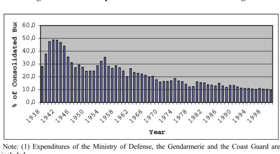
Figure 1: Defense Expenditures as a Share of General Budget

0,0 10,0 20,0 30,0 40,0 50,0 60,0 1938 1942 1946 1950 1954 1958 1962 1966 1970 1974 1978 1982 1986 1990 1994 1998 Year % of Consolidated Bu d

Note: (1) Expenditures of the Ministry of Defense, the Gendarmerie and the Coast Guard are included.

(2) Source: “The Realizations of Budget Income and Expenditures, 1924-1991” published by the Ministry of Finance.

Defense spending is, of course, one of the governmental policies most frequently linked to inflation. Policymakers and analysts have come to realize that security is a more complex issue than simply spending money for defense. For example,

Knorr has noted that the “question of national priorities raised by military demands turns on the relation between the expected utility of satisfying these demands . . . and the expected disutility imposed by opportunity costs” (Knorr,

1977: 192). The defense burden of the general budget of Turkey can be seen clearly in Figure 1. Although the extra budget sources, like Defense Industry Support Fund of Turkey, are excluded in Figure 1, it is obvious that a

considerable part of the budget is devoted to defense expenditures. In addition,

the budget deficit of Turkey increased steadily especially since 1985 (See Appendix B). From these figures, one can conclude that defense expenditure is one of the main reasons for increasing budget deficit in Turkey.

The complex relationship between defense spending and inflation has been of interest to scholars and policymakers at least since World War II. Although concern with the strength and form of such a relationship is not new, the interest has been taken up with renewed enthusiasm in Turkey; because Turkey initiated

an arms industry modernization programme in early 1980 with an estimated cost of 10-12 billion dollars at time of initiation, a policy of attacking inflation yet increasing defense spending to record high levels. Off course, defense spending

does not have a direct relationship with inflation, but on the other hand it has an implicit effect on inflation by increasing budget deficit. As stated above, inflation comes into existence when the government monetizes the budget deficit.

Yet there is no agreement among economists, political scientists, or policy analysts as to the exact nature of the relationship between defense spending and inflation. The thesis will attempt to shed some light on this matter by identifying the alternative views on the relationship between defense spending and inflation

that appear in the literature and subjecting them to empirical examination. While several studies have examined the relationship between defense spending and inflation in different countries, there is not any study which concentrated only on this relationship in Turkey. For this reason, the thesis has a unique importance.

The defense spending and inflation relationship is investigated by using Johansen

Cointegration test for comovement of variables and applying Direct Granger Causality test for predictive ability with data from 1950 to 2001 for Turkey. The empirical results of this study indicate the existence of the significant relationship between defense spending and inflation in Turkey.

It is obvious that there are reasons to believe that the character of the relationship varies across countries. It is also worth noting that there is agreement in the literature that inflation and defense spending are complex phenomena and

disagreement over the best way to measure them (for example, Clayton, 1976; Boulding, 1979; Weidenbaum, 1974). A complete model of inflation will not be developed in this study. Instead the thesis aims to begin to sort out the direction

and extent of the bivariate relationship between defense spending and inflation, as a way of approaching a relatively complex topic. By beginning with simple analytic models, it will be possible to comment on the bivariate policy recommendations found in both the academic and the journalistic literatures. The

thesis also aims to provide the basis for subsequent work on a more complex model focusing on defense spending and inflation.

This thesis hopes to uncover interdependence between defense spending and

inflation and is organized as follows: In Chapter 2, theoretical background and a brief literature survey about budget deficit, money growth and inflation are discussed. The literature review about the relationship between defense spending and inflation is given in Chapter 3. Chapter 4 explains data and methodology.

Chapter 5 contains the empirical findings. Finally conclusion and discussions

CHAPTER 2

BUDGET DEFICIT, MONEY GROWTH AND INFLATION

2.1 Theoretical Background

The main aim of the thesis is to investigate the relationship between inflation rate

and defense expenditures in Turkey. However, the relationship between inflation and defense expenditures is closely related with the relationship between budget deficit, money growth and inflation rate in Turkey. Alternative economic theory frameworks provide different relationships between these variables.

The first one is the quantity theory of money. In the quantity theory of money,

the major factor causing general price level to increase is the quantity of money. There are three basic propositions in the quantity theory of money: 1) quantity of money is exogenous implying that causality moves from money to price instead of vice versa, 2) demand for money is a stable function implying stable velocity

of circulation, 3) the volume of real transaction and output is determined, independently from the quantity of money or price, by real variables such as

factor endowments, preferences and technology (Blaug, 1995). According to the

quantity theory, inflation is a monetary phenomenon and budget deficit may not be inflationary unless it is monetized.

It follows from these propositions that inflation is always and everywhere a monetary phenomenon in the sense that it is and can be produced only by a more rapid increase in the quantity of money than in output. ... Government spending may and may not be inflationary. It clearly inflationary if it is financed by creating money, that is by printing currency or creating bank deposits. If it is financed by taxes or by borrowing from the public, the main affect is that the government spends the funds instead of the taxpayer or instead of the lender or instead of the person who would otherwise have borrowed the funds (Friedman, 1990: 32).

In the three variable system containing inflation, money growth and budget deficit, money is exogenous and determined by the monetary authority and there is no direct link between the size of budget deficit and money growth. Thus,

inflation is created via money supply growth to finance budget deficit and government can obtain seigniorage and inflation tax revenues through its direct control over money creation.

Second theory is the new classical approach, in which, fiscal side of inflationary process is raised in addition to the monetary side. According to the unpleasant

monetarist arithmetic, whether inflation is in the control of monetary authority or not is critically depends on the domination of the monetary policy over fiscal policy (Sargent and Wallace, 1981). If the fiscal policy dominates monetary policy in which the fiscal authority independently sets its budgets, announces all

its current and future deficits and surpluses, determines the amount of revenue

that must be raised through bond sales and seigniorage, and an interest rate on bonds is greater than the economy’s growth rate, then the monetary authority lost its control over inflation and monetary base growth.

Which authority moves first, the monetary authority or the fiscal authority? In other words, who imposes discipline on whom? The assumption made in this paper is that the fiscal authority moves first... Given this assumption about the game played by the authorities, and given our first crucial assumption, the monetary authority can make money tighter now only by making it looser later (Sargent and Wallace, 1981: 7).

This implies that contractionary policy today is higher inflation tomorrow in the long run. Thus, increase in money growth is a natural result of higher budget deficit, so inflation is a fiscal phenomenon.

However, there are alternative theories stressing the significance of institutional

factors and endogeneity of money supply. Portfolio adjustment approach suggests that the link between changes in public sector deficits and changes in the money supply depends on many factors including institutional structure of the economy and nature of the financing decision. This approach takes into account the asset preferences of the public and the liability management of the financial

system. Commercial banks are profit-maximizing entities operating within a specific market setting and have particular risk-preferences. Commercial banks

expand credit if it is profitable. The relevant issue is whether the restrictions on

the banks money creation mechanism are effective or not (Jackson, 1990).

If the demand for credit is price-elastic and if the supply of credit is price-elastic than the expansion of credit, even under penal conditions created by the central bank, must be profitable for the commercial banks. Whether or not a bank deposit multiplier process exits depends crucially upon the portfolio decisions of profit-maximizing banks facing different risks (Jackson, 1990: 119-20).

Proponents of this approach conclude that there is no inevitable link between government deficit and money expansion. In economics with well-developed

capital markets, government deficits need not be financed through the banking system, so there would be no one-to-one relationship between government deficits and money stock.

Another alternative approach is the credit counterparts approach. In this

approach, balance sheets of the four sectors; officials sector, foreign sector, private non-financial sector and financial sector, are used in deriving money supply identity. By using simple national income and expenditure identity, they derived the money stock identity. In this identity, increase in money supply is

equal to the public sector borrowing requirement less sales of bonds to the non-bank private sector plus net external inflows plus increase in non-bank lending to the private sector less increase in net non-deposit liabilities. In sum, credit counterparts approach conceives quantity of money stock determination process

opportunities secure in the knowledge that they can buy in reserves to support

their loan book-what is known as “liability management” (Artis and Lewis, 1990: 5).

Financing budget deficit by selling government bonds or bills to the banks may or may not increase money stock depending on the perception of the newly issued government debt instruments as a rival or not to the private sector

borrowing instruments. In the case of rivalry between public and private debt instruments government borrowing may crowd out the private borrowing and so money stock remain unchanged. If there is no rivalry between them, especially if

banks have excess free reserves, government borrowing only increases the total credit stock and the money stock. In the later case, crowding out of the private borrowing does not occur.

The problem of time inconsistency in monetary policy is also discussed as a factor creating difficulties to the monetary authority to control money supply.

Time inconsistency problem asserts that monetary policy aiming to simulate growth, smoothing the business cycle or stabilizing exchange rates in addition to its prime concern, controlling inflation, will not provide stable money. Not only the path of developments of these multi-targets may contradict but public

expectations take the possibility that monetary authority may deviate from its inflation objective into account. Monetary authority’s credibility may be

destroyed and the stable link between money stock and inflation may be lost

(Neumann, 1996).

2.2 A Brief Literature Survey on Recent Economic Studies

In a study (Alper and Üçer, 1998), authors run an unrestricted vector autoregression to test the predictive content of fiscal against the balance of payments views as well as to find out the impact of inertia and public sector

prices on inflation. In the empirical part of their study they conclude that more than 90 percent of variation in inflation is explained by the past inflation instead of exchange rate depreciation or money growth implying that there is inertia in the Turkish inflation.

In addition, Granger causality tests are also applied to the Turkish data (Abaan,

1993; Ülengin, 1995). For the period 1983-90, Abaan (1993) found bi-directional Granger Causality between currency issued and inflation rate, which implies endogeneity of the currency issued to the path of price. He also found M1 and M3 endogenous with respect to inflation. Interestingly his study

indicated bi-directional causality between M2 and inflation, which also indicates feedback from inflation to M2.

The study by Ülengin (1995) is the application of the multivariate Granger

Causality for the period 1981-92 and two different close circuits of inflationary processes are identified. The first circle is among budget deficit, reserve money and inflation. The budget deficit Granger causes reserve money while simultaneously reserve money Granger cause budget deficit. In turn reserve

money Granger causes inflation and inflation Granger causes budget deficit. Budget deficit increases reserve money growth, rise in money growth increases inflation rate and in turn rise in inflation rate and reserve money increase budget deficit. This process is a self-fulfilling, process, which repeats itself. The second

circle is among reserve money, inflation and exchange rate. There are bi-directional Granger causality between exchange rate and reserve money and, exchange rate and inflation. Increase in either of the variable would start a

self-fulfilling inflationary process.

Another study was related to leading indicators of inflation (Kalkan, et al., 1997). Interbank interest rate and exchange rate were estimated as the strongest leading indicators of inflation. Interestingly, predictive power of TL dominated monetary

aggregates was considerably weak. Generally, Granger causality moves from inflation to TL dominated monetary aggregates. In contrast, the predictive power of foreign currency aggregates and monetary aggregates consisting foreign currencies on inflation were estimated quite high. Lastly, public sector deficit is

Despite its lack of identifying long-run relations, Granger causality gives

important insights to the short-run dynamics of inflations in Turkey. But, it should be noted that findings of all these studies may radically diverge depending on the period coverage and the way that causality applied. The more advanced econometric studies using cointegration is required to identify long-run

equilibrium relations (for example, Yavan, 1993; Koğar, 1995; Tekin, 1997; Metin, 1998).

Yavan (1993) performed Johansen’s Method of cointegration and he estimated the long-run money demand function of Turkey. Even though, four statistically

significant cointegration vectors were estimated, Yavan concludes that the only one of them is interpretable. The interpretable cointegration relation is the money demand function. Money demand was found positively affected from inflation, real growth and interest rates.

Koğar (1995) estimated the long-run money demand function by using quarterly

data from 1978Q1 to 1990Q4 and applying the Johansen’s cointegration method. She also found a positive long-run effect of real income on money demand. She estimated the coefficients of inflation and interest rates in the money demand as negative.

Tekin’s (1997) thesis on the subject, which is the application of Johansen’s

conclusion is that budget deficit is the main cause of inflation in Turkey. She

also found budget deficit weakly exogenous to the system. Another conclusion is that inflation determines the currency growth rate in the long run. This finding supports the endogeneity of the money supply arguments. She also performed a trivariate cointegration and she estimated the inflation and the reserve money as

endogenous and the budget deficit weakly exogenous to the system. Finally, she concludes that inflation is not a pure monetary phenomenon in Turkey but a fiscal problem.

Lastly, Metin’s (1998) study on the similar set of variables identified 3 significant

cointegration relations in which one is inflation equation. She used quarterly data of Turkey over the 1950-87 period with real growth rate, scaled base money, budget deficit and inflation rate in the variable space. In the inflation equation, inflation is positively related to the scaled budget deficit and scaled base money.

CHAPTER 3

LITERATURE REVIEW

3.1 Different Views on Relationship between Defense Spending and Inflation

There is no widespread agreement about the existence and form of the relationship between defense spending and inflation. While many observers

argue that defense spending has a clear and direct causal effect on inflation, three other possibilities exist, and each has its own proponents and supporting rationale. Not only may defense spending affect inflation but also inflation may

affect defense spending; in addition, each may affect the other in a two-way relationship or there may be no relationship between defense spending and inflation. The general arguments that have been presented for each of these possible relationships are reviewed below.

3.1.1 Defense Spending Affects Inflation

The financing of defense expenditure has an important impact on its

expenditures have the highest chance of creating an inflationary environment.

At the opposite extreme is taxation which directly limits private demand.

It is commonly argued that defense spending is an economic instrument, a macroeconomic tool. In USA, The Council of Economic Priorities notes simply

that military spending is the largest mechanism available to the federal government for stimulating the economy with purchases (DeGrasse, 1983: 153). That is why policymakers often perceive that defense spending is useful in affecting both recession and inflation. The main assumption is the widespread,

fundamental belief that defense spending is inflationary. The usually well-paying defense contractors create increased domestic purchasing power that is not met by increase in domestically produced civilian goods. When demand or

purchasing power exceeds supply in any economic system, the requirements for the classic definition of inflation have been met (Hartman, 1973). Military spending by its non-productive demand generating nature is inherently inflationary. For example, this has been the pattern in USA historically:

We have had four periods of extreme inflation and deflation since 1800- all produced by war. The Civil War and World War I each doubled prices. World War II increased prices by 50 percent. The Korean War further increased the cost if living by about ten percent (Clayton, 1970: 63).

Several observers (Calleo, 1981; Steel, 1981) link defense spending to domestic and foreign policies that overextend, due to the conscious efforts of those

pursuing ambitious policies who are unwilling to tax or to cut back expenditures

of a nation’s resources in other areas, thus leading to inflation.

Similar arguments are found in discussions linking war to inflation (Hamilton, 1977; Stein, 1980; Melman, 1970). Without taxation to cover the costs of

warfare, war is found to be clearly inflationary: “Wars and revolutions have been the principal causes of hyperinflation in industrial countries in the last two centuries” (Hamilton, 1977: 18). A Congressional Budget Office report indicates that when the United States rapidly expanded defense expenditures in past war

situations (using 1917, 1941, 1950, and 1965 as points of comparison), a substantial increase in inflation followed (Sandler and Hartley, 1990). The average inflation rate for the three-year periods preceding those dates was 3.55%,

compared to a 7.3% average inflation rate for the three-year periods subsequent to those dates.

Furthermore, Hamilton (1977) and Stein (1980) point out that inflation is both

much the easiest way to pay for war and a policy preferred to taxation. Resources for defense spending can be provided from increased taxation, cuts in non-defense spending, and/or deficit spending. Thus one alternative is to cut government spending in other areas, such as social services. This is the focus of

the literature on the opportunity costs or trade-offs of defense spending. While the results differ somewhat from country to country, several studies demonstrate some trade-off between peacetime defense spending and certain forms of social welfare expenditure, investment, and/or private consumption (Caputo, 1975;

Russett, 1970, 1969; Peroff and Podolak-Warren, 1979; Smith, 1980; Deger and

Smith, 1983; DeGrasse, 1983).

Later studies qualify the earlier findings of peacetime defense spending and trade-offs. Investigating trade-offs in the United States, the United Kingdom,

France, and the Federal Republic of Germany during the 1948-1978 period, it is found that there are no trade-off patterns in the short term (meaning yearly changes in spending levels) (Domke, et al., 1983). Trade-offs are discovered in long-term trends, but they occur only in periods of war or of postwar

reconstruction. Russett (1982), looking at the effects of rates of change in military spending on federal health and education expenditures in the United States, found no systematic trade-off. Later, Mintz (1989) replicated Russett`s

(1982) with less aggregated data on military spending. Mintz`s analysis confirms Russett`s (1982) and Domke, Eichenberg, and Kelleher`s (1983) findings of no trade-off in the period from 1947 to 1980. All these researches, so far, consider only the direct affects of military spending but also there is an indirect affect to

be considered (Mintz, Huang, 1991). Their findings confirm earlier findings reported in above researches of a lack of evidence for a direct guns-butter trade-off but show the existence of an indirect effect between military spending and education spending. In other words, they found that military spending crowds

out investment, which slows down economic growth, thereby putting pressure on education spending. They also indicated that it took about six years for such an indirect trade-off to be realized. In Turkey, it is found that while military spending decisions are made independently of health and education expenditure,

there are trade-offs between defense and welfare spending (Sezgin and Yıldırım,

2002). While the trade-off is negative between defense and health, it is positive between defense and education.

The view that defense spending is responsible for inflation is also based on

arguments that the economic nature of military goods leads to inflation (Dumas, 1977; Melman, 1978; Thurow, 1981; Franko, 1982). The central point is that defense spending is nonproductive, unlike other forms of economic activity (including other types of government spending). It is argued that defense

spending generates no additional purchasing power. The complex economic processes behind this view are summarized by Fallows (1981: 7):

The first principle is that defense spending is inherently more inflationary than other kinds of government spending. . . . The problem with military spending, simply put, is that it adds to the demand for goods without adding to the supply. . . . Military and non-military spending add to the demand; non-military spending does not add to supply.

The manner in which the military procures goods and services is also considered to be inflationary. For example, Melman (1978) argues that firms serving the military run their businesses on a cost-maximizing basis and that this becomes a model for increases in costs and prices in the civilian sector as well. Because

there are many military needs that can be supplied by only a few firms, and for this reason Schultze (1981) argues that heavy and rapid military spending can strain the industrial base by leading to bottlenecks and shortages. The danger is the adverse affect such bottlenecks will have on productivity.

The effect of defense spending on the general price level can be transmitted

through changes in aggregate demand and/or aggregate supply. On the demand side, rapid defense buildups contribute to acceleration of nominal demand growth that will affect inflation adversely if not offset by tax increases or monetary growth reductions. In this respect, the demand side effect of increased defense

spending is no different from that of other government expenditures (Schultze, 1981).

A related argument focuses on the short-term effects of switching expenditures

from the civilian to the military sectors of the economy (DeGrasse, 1983; Franko, 1982). Defense spending increases the demand for labor, machinery, and capital as supplier firms gear up for increased production. In the short-term, the

aggregate supply of labor, machinery, and capital is more or less fixed. Therefore, in the short-term, a rapid increase in defense spending should produce an increase in wages, prices, and rents. Thus, for given demand pressure and inflation expectations, defense spending has a potential supply side effect on the

rate of price inflation similar to the effect of the oil price shocks of the 1970s (Capra, 1981). Even in the long term, the supply of certain factors (e.g., trained engineers) will not respond quickly to increased demand, and there may be some long-term effects. In addition, one can expect those industries in the civilian

sector that require the same inputs as firms in the military sector to face severe shortages of supply which they are likely to pass on in the form of sharply higher prices. This is what DeGrasse (1983) calls “sectoral inflation”. Finally, civilian technological progress is likely to be hindered by the diversion of capital and

expertise to the military sector, thus reducing the ability of the civilian sector to

offset rising production costs through technological innovation.

It is also argued in the literature that defense spending generates a greater public debt, which is inherently inflationary. For example, DeGrasse (1983) sees the

Reagan administration’s fiscal policies leading to large federal deficits due mostly to defense spending, which are expected to exceed the peak deficits of the Vietnam War and thus could stimulate inflation. The deficits caused by defense spending could produce more inflation if it is financed by increasing money

supply. Şimşek (1993) states that if the military expenditure is the one of the main causes of budget deficit, finally, it causes inflation by money creation.

In other words, defense spending can lead to inflation through deficit spending if the economy has idle capacity at the time deficits increase and/or deficit spending is attractive as an alternative to cutting back nonmilitary expenditures because of the desire on the part of the government to stimulate the economy and its relative

unconcern with the possible inflationary consequences.

Vitaliano (1984) tested the hypothesis that rapid defense buildups contribute to inflation and finally he found that defense spending has a discernible influence on

the rate of inflation. His results indicate that "there appears to be no perceptible impact on the rate of price inflation separably attributable to defense spending" (Vitaliano, 1984). The most troublesome aspect of Vitaliano's work is his use of the nominal rate of interest as a proxy for the expected inflation rate. This causes

an error-in-variable bias (i.e., bias due to misspecification of explanatory

variables) if the expected real rate is not constant (Wilcox, 1983). In this case, ordinary least squares (OLS) estimators will be biased and inconsistent, and the classical test of hypothesis produces misleading results (Nourzad, 1987). Even if the model did not suffer from this problem, the estimates still would be biased

and inconsistent due to the simultaneous equation bias that results from the interaction between inflation and the nominal interest rate. Nourzad (1987) corrects this bias by applying a second order Almon-distributed lag structure for the expected inflation rate. In contrast to Vitaliano's findings, Nourzad (1987)

finds defense spending to have an inflationary impact. Since all other factors are common between the two models, the difference in the conclusions is attributable to the different measures of the expected inflation rate.

The effect of increased defense spending on the balance of payments is yet another way in which it can affect inflation. The component of defense spending that is actually spent abroad (e.g., for military personnel and facilities) contributes

to payments deficits. The effects of the payment deficit on inflation depends on how big the deficit is and how it is financed. A large deficit can induce downward revaluation of the currency exchange rate and thus make imports more expensive and exports more competitive. The increased cost of imports and the

increased price of goods exported, due to increased foreign demand, may result in some increases in the overall rate of inflation. A large deficit, if financed by domestic borrowing can actually be deflationary, to the extent that it diverts capital away from domestic production and reduces aggregate demand. In

addition, if import controls are introduced to reduce a balance of payments

deficit, the end result may be deflation rather than inflation.

Finally, if the country with a large deficit is a key currency country (a country whose currency is widely used by many nations as a means of transacting

international business), that country can simply continue to run a deficit for a time and justify it in terms of the need for currencies to enhance global liquidity. It is obvious that this strategy will have a negative effect on the exchange rate of the key currency country eventually, but historically, key country currencies have

been able to run balance of payment deficits for quite some time before running into this difficulty.

3.1.2 Inflation Affects Defense Spending

Several researchers (Kaufman, 1972; Capra, 1981) argue that inflation is a

powerful factor in rising defense expenditures. As inflation increases, it has an impact on costs and cost-overruns, and it cuts into the purchasing power of the defense dollar. Proponents of a larger defense budget often argue that increases in defense spending are required to compensate for inflation and maintain the

targeted level of real defense spending. This is a kind of indexing of defense spending to inflation that creates a causal link between the two as long as it is consistently done over time. There are international elements to this relationship as well. It might be necessary to increase spending for overseas facilities in allied

countries to which large states such as the United States have exported their

domestic inflation. In addition, a state may increase defense spending to match an opponent whose own defense spending has increased due to inflation. Thus we must consider the possibility that inflation is a major determinant of increased defense spending. On the other hand, it is conceivable that inflation may

stimulate cuts in defense spending as governments use defense spending as an inflation-reducing device.

3.1.3 Two-Way Relationship between Defense Spending and Inflation

If defense spending does have an impact on inflation, then many observers would

entertain the prospect that the relationship between defense spending and inflation involves a complex two way feedback process. Indeed, most of the literature is consistent with the idea of either a one-way relationship wherein defense spending affects inflation or a complex two-way feedback relationship

between defense spending and inflation.

3.1.4 No Relation between Defense Spending and Inflation

It is obvious that defense spending and inflation do not have a direct relationship. Publications by several researchers also emphasize that defense spending and inflation do not have any meaningful relationship. One view, illustrated by a

Merrill Lynch Economics analysis (Forbes, January 21, 1980), suggests that

non-defense policies can and do produce a strong private sector and national economy as a whole, and thus enable the economy to absorb higher defense spending without increased inflation. Such policies include reduced government regulation, cutting spending in other areas such as the social welfare field, tax

cuts and growth-oriented tax changes, and policies to take advantage of slack capacity in the economy. The main factor in regard to inflation would be how the increased defense spending would be financed. The Congressional Budget Office report (Sandler and Keith, 1990) similarly notes that a slow recovery and

slack in the economy will permit increased defense spending without inflation in the short term.

Schultze (1981: 1) observes: “The United States is fortunate in having an economy, that, with proper policies, can adjust to about as high or low a level of defense spending as the nation and its leaders think is appropriate.” He goes on to discuss the special problems that arise over the short run from a rapid increase

in defense spending. He also attempts to dispense with the argument that defense spending is inherently inflationary. He argues that defense spending is no more inflationary than any other type of government spending (1981: 2): “In sum, government purchases do not add to market supply in the economic sense of the

term. Hence taxes must be levied. But the military nature of the goods is absolutely irrelevant.” He also notes that increases in defense expenditure, as a percentage of GNP need not be inflationary; they would be inflationary only if those increases came at the expense of investment rather than consumption.

Several publications present evidence that there may be no meaningful positive relationship between defense spending and inflation. Calleo (1981: 782) notes that prices in the United States have risen approximately 177% since 1960. At the same time, other analysts have demonstrated that defense spending in real

terms in the United States has been falling for the same time period. For example, Clayton (1976) examines six different methods of measuring U.S. defense spending: (1) Department of Defense [DoD] method, (2) DoD method plus retirement pay, (3) Census Bureau method, (4) Joint Economic Committee

method, (5) DoD Deflator method, and (6) Federal Purchases Deflator method. He concludes that no matter which method is used, defense spending in real terms has been falling.

Boulding (1979) also presented additional supporting evidence for the no relationship hypothesis. He divides the post-World War I era into four periods: (1) the “depressed OS," characterized by enormous deflation; (2) World War II,

marked by suppressed inflation and huge deficits; (3) the “long boom” of 1948-1969, marked by moderate deficits and moderate inflation; and (4) the “growing crisis” since 1969, marked by large and increasing deficits and accelerating inflation. Defense spending was negligible in the first of these periods, while in

the second it accounted for the budget deficits and inflation. In the third period, after the Korean War, defense spending does not appear to be closely related to government deficits or to inflation. Finally, in the fourth period, while the inflation had been increasing, defense spending declined as a percentage of GNP:

“It cannot be blamed for the increasing deficit, and it is hard to blame it for the

increased rate of inflation” (Boulding, 1979: 94). Moving on to a comparative perspective, Boulding examined data from Japan, West Germany, Italy, France, and Canada, and demonstrated the weak relationship between defense spending as a percentage of GNP and the rate of inflation.

Employing a Granger causality framework like in our study, Payne (1990) finds no evidence to suggest that defense spending causes inflation. In a research made in 1995, using a closed economy IS-LM model with an expectations-augmented

Phillips curve, no significant relationship between growth in defense spending and the inflation rate is found (Sahu et al, 1995). Unlike prior studies, non-defense spending included in the analysis. Neither non-defense nor non-non-defense

spending is found to have a statistically significant impact on inflation.

In sum, much has been written about the link between defense spending and inflation but little agreement has been reached about how (or whether)

government purchases of military goods and services affect and are affected by price changes. It can be seen from the four relationships outlined above. Questions have been raised about the rapidity of the increase in defense spending and the ways in which it is financed. Several recent observers have noted the

differential impacts of defense spending in the short and long terms. In addition, many studies recognize the possibility that the character of the relationship varies across countries. For example, the financing of defense spending may have a

greater (or lesser) effect on investment, or defense spending may create more

CHAPTER 4

DATA AND METHODOLOGY

4.1 Data

“Statistical Indicators, 1923-2002” published by the State Institute of Statistics provides data for inflation (consumer price index). The defense expenditures of

Turkey are taken from the various issues of SIPRI yearbooks (Swedish International Peace Research Institute). Inflation data go back to 1938, but data for defense expenditure are available for 1950 and after. Thus, the data used in

this study comprise the years 1950-2001. In addition, annual data are used in the thesis.

In econometric studies, it is important to use the right data to get reliable results.

However, it is hard to reach the right defense expenditure data. One main obvious reason is that expenditures of the Ministry of Defense, the Gendarmerie and the Coast Guard are included in the budget, but procurement expenditures implemented by the Undersecretariat of Defense Industry and financed by the

defense expenditures partly financed by extra-budget sources, like the Defense

Industry Support Fund of Turkey, actual defense expenditures are underestimated by the defense expenditures item in the government budget (i.e. the budget of the Defense Ministry). The data from SIPRI yearbooks are used as the all previous studies did.

In addition, there is no agreement concerning the form of data set to be used. Thus, it is an important issue for empirical studies whether or not to use levels of military expenditure or shares of military expenditure out of GDP. Brauer and

Dunne (2002) argue that results of the empirical studies appear to depend whether level or share are used. Hartley and Sandler (1995: 213) argue that if the variables are used in levels, the nature of the demand for military expenditure is

better explained. Thus, the level data for the defense expenditures is used in this study.

4.2 Unit Root Tests

In time series stationarity of the variables is important. Ordinary regressions including non-stationary variable may lead to misleading results. Regressions

including non-stationary variables could have a non-stationary error term, which may calculate high R² even though there is no link between the variables. Standard testing procedures became inapplicable to these regressions. In other words, coefficients of the estimate in the non-stationary process do not converge

in probability to constants, distributions of F-and t-statistics diverge, DW

statistics converges in probability to zero and R² has a non-degenerate limiting distribution as sample size tends to infinity (Mills, 1993). This is known as the problem of spurious regression (Hendry, 1986; Davidson and MacKinnon, 1993).

It is argued that differencing a variable is a way of making it stationary. Let’s assume that Xt is a non stationary variable in which differencing d times makes is stationary than we may conclude that Xt is integrated of order d (Xt ~ I(d)).

Non-stationarity of a variable may simply be tested by using Augmented Dickey-Fuller test (ADF) (Dickey and Dickey-Fuller, 1979; 1981). In this test, presence of unit root should be tested at level form first. If ADF test finds the variable

non-stationary, the same test should be performed for the first difference of a variable. If first difference of a variable is also found non-stationary, the same test should be applied for the second difference of the variable. This process is repeated up to the rejection of the unit root hypothesis (null hypothesis).

ADF test is the OLS regression of the model:

∑

The model estimated above is used in testing the presence of unit root at the level

of the dependent variable added to the model in order to eliminate the

autocorrelation, T is trend. The null and alternative hypotheses are:

0 : ₀ 0 γ = H 0 1:γ H

‹ 0

ADF test is simply significance test for the coefficient ofX_t−1,γ₀, in the regression. T-value of Xt-1 is used in this test procedure but critical values are

different. Under the γ₀ ≥0 condition Xt is non-stationary, so even asymptotically its distribution diverge form the standard students t-distribution. Since, these statistics do not have the standard-distribution they are referred as τ statistics (Davidson and MacKinnon, 1993). Critical values presented by

MacKinnon (1991) are the appropriate one. Null hypothesis γ₀ =0 is implying that there is a unit root in the data generating mechanism of a variable.

Alternative hypothesis is that γ₀ significantly different from zero. If calculated t-value of γ0 is below the critical value than Xt is stationary. If not Xt is

non-stationary.

In the case of I(1) variables their first different should be used in regressions. Otherwise their estimates became unreliable. Using the difference of a variable

instead of its level form may solve the problem of unit root but valuable long-run information lost from the models. Regressions with only difference form of the

variables represent short-run relations but not the long-run equilibrium dynamics.

This later point, promoted the development of error correction models which incorporates long-run equilibrium relation into the short-run models.

In addition, one has the choice of including a constant, a constant and a linear

time trend, or neither in the test regression. The choice here is important since the asymptotic distribution of the t-statistic under the null hypothesis depends on the assumptions regarding these deterministic terms. There remains the problem whether to include a constant, a constant and a linear trend, or neither in the test

regression. One approach would be to run the test with both a constant and a linear trend since the other two cases are just special cases of this more general specification. However, including irrelevant regressors in the regression reduces

the power of the test, possibly concluding that there is a unit root when, in fact, there is none. The general principle is to choose a specification that is a plausible description of the data under both the null and alternative hypotheses (Hamilton, 1994: 501). If the series seems to contain a trend, one should include both a

constant and trend in the test regressions. If the series does not exhibit any trend and has a non-zero mean, one should include a constant in the regression, while if the series seems to be fluctuating around a zero mean, one should include neither a constant nor a trend in the test regression.

In this study, the regression includes both constant and trend. The lag lengths are chosen according to Akaike Criterion and Schwarz Criterion.

4.3 Johansen’s Cointegration Estimation Method

The problem of unit root and the problem of identifying long-run equilibrium relations when variables are not stationary were the major econometric problems before the development of cointegration. Cointegration analysis offers a way of

incorporating long-run relation into a short-run model. The main idea behind cointegration comes from the idea of stationarity. If variables are non-stationary, than their linear combination should be non-stationary also. If linear combination of a non-stationary series is stationary than this imply a kind of tendency of these

variables to adjust any deviations from the long-run equilibrium condition. Error term of the linear combination of these variables diminishes as time passes and goes to zero as time goes to infinity. Error term of the linear combination is the

same as deviations from the long-run equilibrium; so as time goes infinity, deviations from the long-run equilibrium go to zero.

One of the formal definitions cointegration is:

The components of the n-dimensional vector Zt are said to be cointegrated of order d,b denoted Zt~CI(d,b) if (i) all components of Zt are I(d); and (ii) there exist at least one vector α(≠0)such that

. 0 ), ( ~ − > ′ = Z_t I d b b t α

ν The vector α is called the cointegrating vector (Engle and Granger, 1987: 253).

There are number of different ways of testing and estimating cointegration

relations. One of them is the well-known residual-based approach by Engle and Granger (1987). In this method, cointegration relation is estimated by OLS and

than the standard unit root test is applied to the estimated residuals, however with

different critical values1. In the theory of cointegration, residuals of the cointegration relation should be stationary. Non-stationarity of the estimated residuals, on the other hand, concludes the non-existence of a long-run relation. Impossibility of testing and estimating more than one-cointegration relation is the

main weakness of this method. Later, Johansen and Juselius (1990) proposed an alternative method of testing and identifying cointegration vectors when there is more than one cointegration relation. This method is based on the estimation of

VAR by maximum likelihood. The method is based on VAR (m):

t i t m i i t T CZ Z =α+β + ₋ +ε =

∑

which can be reparametrised as:

t m t i t m i i t T Z Z Z =α +β + Π ∆ +Γ +ε ∆ − _{− −} =

∑

Above formulation is known as reparametrised VAR (m) in the VECM form (Johansen and Juselius, 1990) in which T is the time trend. In this regression there are n number of variables and

) ... ( _{1 2 i} i =− I−C −C − −C Π

1 _{Since the null hypothesis is that parameters are estimated from the spurious regression, their}

asymptotic distribution is not the same as the distributions used in the standard unit root tests. These are known as Engle-Granger tests.

) ... (I−C₁−C₂− −C_m − = Γ β α ′ = Γ

in which α is the adjustment matrix and β is the matrix of cointegration vector coefficients. Rank of a matrixβ determines the number of cointegration relations. If the rank of β is zero than there is no cointegration relations. If rank of β is equal to the number of variables, than all variables are stationary, and again implying that there is no cointegration relation. If 0 ≤ rank(β) ≤ n than there exist a rank (β)number of cointegration relations.

The test statistic is calculated from the residuals of the auxiliary regressions.

∑

∑

∑

LR test statistics of at most m cointegration vectors is:

∑

where λ)_r+_1,...,λ)_nare the n-r smallest eigenvalues of 01 1 00 10 ∧ ∧ ∧) )− ) _{with respect to} . 11

∧) This is known as the trace test statistic.

) 1 (

2 ₁

max =− InQ=−TIn −λr+

λ )

is known as the maximum eigenvalue test which is based only on the r+1’th

eigenvalue. The null hypothesis in these LR-tests is that λr+1 =λr+2 =...=λn =0, ) )

)

implying that n-r unit roots exist. Sequence of hypothesis starting with the hypothesis of n unit roots is applied to determine the cointegration rank. If this

hypothesis is rejected, than, at least one cointegration relation exist, λ)₁ >0. The test is proceeded by applying the hypothesis λ)₂ =λ)₃ =...=λ)_n =0. Rejection of this hypothesis is also implies thatλ)₂ >0, and so forth. This process is carried out up to the non-rejection of the null hypothesis. At the non-rejection of the null hypothesis, the number of significant cointegration relation(s) is/are identified (Hansen and Juselius, 1995).

Long run exclusion test is applied to test the significance of the each variable in

the long run cointegration space. In the null hypothesis, β coefficients of the variables are set equal to zero. Rejection of the null hypothesis implies the

significance of the variables in the long-run relation.

Weak exogeneity test, on the other hand, is the test on the α coefficients of the variables in the cointegration equations. In the null hypothesis, α coefficients are set to zero. Rejecting the null hypothesis implies the adjustment of the variables to the deviations from the long-run equilibrium.

4.4 Granger Causality Test

The notion of Granger causality is based on a criterion of incremental forecasting

value. A variable X is said to “Granger cause” another variable if “Y can be better predicted from the past of X and Y together than the past of Y alone, other relevant information being used in the prediction” (Pierce, 1977).

Sims (1972) has shown that a necessary condition for a variable X to be exogenous to another variable Y is that Y fails to Granger cause X. Therefore, tests for Granger causality are valuable tools in the empirical analysis of

economic processes. Indeed, in economics, tests for Granger causality are becoming recognized as essential steps in model building (Sargent 1976, 1979, 1981)-steps that provide useful information about the reasonableness of

alternative structural representations (Hernandez-Iglesias and Hernandez-Iglesias,

1981).

For the simplest bivariate case, Granger causality can be operationalized in the following way: Consider the process [Xt, Yt], which we will assume to be jointly

covariance stationary. Denote byX and t Y all past values of X and Y, t

respectively. Let all past and present values of these two variables be represented

as Xt andYt. Define ( )

2 _{X Z}

t

σ as the minimum predictive error variance of Xt, given Z, where Z is composed of the sets

[

]

‹

II. Y causes X instantaneously: 2( , )

t t tY X X σ

‹

‹

‹

IV. Independence: X and Yare not causally related:

) , ( 2 t t t X Y X σ = 2( , ) t t t X Y X σ = 2( ) t t X X σ and ) , ( 2 t t tY X Y σ = 2( , ) t t tY X Y σ = 2( ) t tY Y σ

For instance, in case I the minimum predictive error variance for Xt is smaller

when the past values of Y, Y , are included than when the minimum predictive t

error variance is calculated solely on the basis of X . When the preceding result _t

obtains and, at the same time, X Granger causes Y, we have feedback or case III.

In case II, it is said that instantaneous causality is occurring. In other words, the current value of Xt is better predicted if the present value of Yt is included in the prediction than if it is not.

The definition can be formulated in terms of either the moving average or autoregressive form of the (covariance stationary, purely non-deterministic) bivariate system. Each representation, in turn, suggests an alternative test for Granger causality. In this study, the “Direct Granger Method” which is a second

procedure for assessing Granger causality is applied. To implement this approach, one expresses autoregressive representation of the bivariate system in the form below. Let Xt, Yt be two stationary time series with zero means

(Granger, 1969): t t i i t t X Y a X = + ∞ ₋ + = ∞ = −

∑

∑

∑

∑

where a and b are shocks to the system at time t, neither at nor bt is autocorrelated, and at and bs are uncorrelated for all t and s. A finite number of

lags are chosen for the summations on the right sides of the two equations. Then

ordinary least squares regression is employed to estimate above equations

separately. The test of the hypothesis that the π₁₂ parameters are jointly zero tells us whether Y Granger causes X whereas a test of the hypothesis that the π₂₁ parameters are jointly zero indicates whether X Granger causes Y. If both hypotheses are accepted, we conclude X and Y are Granger independent; if both are rejected, there is Granger feedback between X and Y. The familiar F statistic

usually is employed in making these determinations.

The results of Granger causality tests depend critically on the choice of lag length. If the chosen lag length is less than the true lag length, the omission of

relevant lags can cause bias. If the chosen lag is greater than the true lag length, the inclusion of irrelevant lags causes estimates to be inefficient.