;; jyjj, Λ* ‘'■?t\f!’:^í^ \ ıi->^·· ip w M ♦^•■*—Nlif^v-W *«4<Wi» Λ ■. . -u t '^'V· «I w U·*,, 4ı^· ·, f ı. ■ . ·■' Λ-^ί.«' - · ■' f·* S J ^ â s r
iA
3TB
9Tile kelfil iontihip Between Stock Returns and Inflation in Turkey 1987-isy3
A Thesis Submitted to the Department of Management and the Graduate School of Business Administration
of Bilkent University
in Partial Fulfillment of the Requirements for the Degree of
Master of Business Administration
OSMAN N. TUZUN
И й
5 9.O b . S .А !>
I certify that I have read this thesis and in my opinion it is fully adequate in scope and in quality, as a thesis for the degree of Master of Business Administration.
I certify that I have read this thesis and in my opinion it is fully adequate in scope and in quality, as a thesis for the degree of Master of Business Administration.
Doç. D r . Gülnur Muradoglu
I certify that I have read this thesis and in my opinion it is ful]y adequate in scope and in quality, as a thesis for the degree of Master of Business Administration.
Dr. Nilüfer Üşmen
Approved by the Graduate School of Business Administration.
A H s T R A C T
'L'lici k a l a t l o n s h i p Betweiaii I n f l a t i o n an d S t o c k R e t u r n s i n T u r k e y
OSMAN N. TüZüN MBA in Management
Supervisor : Doç.D r . Gülnur Muradoglu February 1994, 40 pages
■L'ljis study investigates the existence of a negative relationship between real stock returns and inflation, which is observed in other industrialized countries, and a possible explanation for this relationship, in Turkey. This relationship between stock returns and inflation is tested in the light of Kama's "Proxy Effect Hypothesis". This hypothesis suggest that the negative relation between stock returns and inflation is in fact proxying for a more fundamental relationship between real stock returns and real activity.
The empirical investigation of the data revealed that the there is a significant negative relationship between forecasts of real activity and inflation. Also the results suggest that there is a positive, although insignificant, relationship between real stock returns and real activity. These two results can be combined to state that the "Proxy Effect Hypothesis" also holds for Turkey.
Keywords: Expected Inflation, Unexpected Inflation, Stock Returns, Real and Nominal Return, Real Activity Growth Rate, Base Money Growth Rate.
Ö Z E T
Hisse Senedi Getirileri ve Enflasyon Arasindaki ilişki
OSMAN N. TüZüN
Yüksek Lisans Tezi, isletme Enstitüsü Tez Yöneticisi : Doç. D r . Gülnur Muradoglu
Ocak 1994, 40 sayfa
Ut. çalisuta, hisse senedi getirileri ve enflasyon arasindaki, diğer s^ıııayilesmis ülkelerde gözlenen negatif ilişkinin varligini ve bu ilişkinin nedenlerini ara tirmaktadir. Bu ilişkinin arastirilmasi sirasinda. Fama [6]'nin, hisse senedi getirisi ve enflasyon arasindaki negatif ilişkinin aslinda daha temel bir ili kinin, yani hisse senedi getirisi ve reel aktivite arasindaki ilişki sonucunda oluştuğunu ileri süren, "Vekalet Etkisi Hipotezi" kullanilmaktadir.
Bu hipotez paralelinde bilgilerin değerlendirilmesi sonucunda, enflasyon ve reel aktivite arasinda belirgin negatif bir ilişkinin bulunduğu gözlemlenmi tir. Ayrica, bu ilişki kadar kesin olmasa da. Vekalet Etkisi Hipotezi'nin de öngördüğü gibi, hisse senedi reel getirileri ve reel aktivite arasinda pozitif bir ilişki olduğu da gözlemlenmi tir. Bu iki sonuca dayanarak "Vekalet Etkisi Hipotezi" 'nin Türkiye'de de geçerli olduğu sonucuna varılabilir.
Anahtar Kelimeler ± Beklenen Enflasyon, Beklenmeyen Enflasyon, Hisse Senedi Getirisi, Gerçek ve Nominal Getiri, Reel Aktivite Büyüme Orani, Para Tabani Büyüme Orani.
Acknowledgement s :
I would like to express my gratitude to Dr. Gulnur Muradoglu for her invaluable supervision during the development of this thesis. 1 would also like to express my thanks to the Management Department of Bilkent University for providing me with the necessary background through the MBA program.
TABLE OF CONTENTS Abstract Ozet Acknowledgements Table of Contents
11
111 I V 1. Introduction 2. Literature Survey 3. Methodology 3.1 Monetary Sector 3.2 Real Sector 3.3 The Data- Real Stock Return “ Actual Inflation Rate - Expected Inflation Rate - Base Money Growth
- Real Activity Growth Rate
9 13 14 15 15 15 16 16 4. Results 17
4.1 Characteristics of The Data 17
4.2 Inflation, Interest Rates, Money And Real Activity 18 4.3 Real Stock Returns, Real Activity, Inflation And Money 23
4.4 Assumptions TVnd Limitations 24
5. Conclusion References Appendices
A. Regression results of inflation on past and future six levels of Money Growth
six, current
B. Regression results of inflation on past six, current and future six levels of Industrial Production Growth
26 28 31 A1 A2 IV
1. Introduction ;
Since 1980, Turkish economy has witnessed several milestones of financial liberalization. Examples of this rapid improvement are the convertibility of Turkish Lira, establishment of a market oriented economy and may be the most important one is the establishment of Istanbul Stock Exchange (ISE) at 1986. Although it has been only seven years that ISE is established, it is being promoted as one of the promising markets of the world.
Despite such developments, one of the failures of financial liberalization is the continuing high level of inflation. Although ISE is a rapidly developing market, whether the high rate of continuing inflation has a negative effect on stock returns is a discussion issue. Especially for the individual and foreign investor it is very important to see the relationship between stock returns and expected-unexpected inflation since high level of inflation and changing government policies causes uncertainty in the economy.
The effect of inflation on stock returns has raised the interest, especially during the last decade, because financial assets are perceived as hedges against inflation. A high number of studies have revealed a negative relationship between returns on common stock and inflation in US and also in other industrialized countries. These studies also found a consistent negative relation between stock returns and expected inflation, as measured by short-term interest rates.(Ex. Fama and Schwert
[8], Schwert [17], Fama [6], Solnik [18], Gultekin [12] etc,)
These results seem to conflict with the commonly accepted view that stock returns should be positively related to both expected and unexpected inflation. Some researchers (Fama [6] , Mandelker and Tandon [15]) have argued that this anomalous
relationship is "spurious" and that it proxies for more fundamental relationships between stock returns, real activity variables, and money.
In a country like Türkiye, where unstable economic conditions and government intervention are present, it is very important, for any type of investor, to see the effects of economic variables on the returns of investment instruments.
In this study, I will test the "proxy hypothesis" so as to see whether the negative relationship between common stock returns and inflation is in fact proxying for other relationships such as the relationship between stock returns, real activity variables and money.
The rest of this thesis is organized as follows : The first section presents a summary of related literature, the second section presents the data and the methodology used, the third section presents the findings and finally the last section will discuss the findings and conclusions.
2. Literature Survey :
The last three decades has witnessed a period of historically high rates of inflation all around the world. This period of sustained inflation has gathered interest of financial economists on the effects of inflation on corporate profits and stock prices and also on the validity of Fisher Effect.
The original idea of relating the nominal interest rate to expected inflation is commonly attributed to Irving Fisher (1930) . Fisher hypothesized that the nominal interest rate can be expressed as the sum of an expected real return and an expected inflation rate. Formally,
R = E(r) + E('P;+ E(r)E(P)
where R is the nominal return of on an asset, P is the rate of inflation, r is the real rate of return and E is the expectations operator.
As a monetarist, Fisher also believed that the real and monetary sectors of the economy are largely unrelated. He hypothesized that the expected real rate is determined by real factors and is independent of the expected inflation rate. This hypothesis, known as the Fisher Hypothesis about interest rates can be generalized to all assets in efficient markets.
Fauna and Schwert [4], has studied the Fisher Effect to see
the extent to which various assets were hedges against the expected and unexpected components of inflation, in US, They used the following regression model :
R = a + b E ( P ) + c [ P - E ( P ) ] f g
t t t t t
where unexpected component of inflation is simply defined as the actual inflation at time t minus the expected inflation rate af
the beginning of time t. They found that US government bonds and bills were a complete hedge against inflation, and private residential real estate was a complete hedge against both expected and unexpected inflation. The most anomalous result was that common stock returns were negatively related to the expected component of inflation.
Fcuna [6], hypothesized that "negative relations between
stock returns and inflation are proxying for positive relations between stock returns and real variables like capital expenditures, the average real rate of return on capital and output, which are more fundamental determinants of equity values." He used a rational expectations view of money demand theory to study the inflation process by taking into account changes in interest rates, current and past money growth rates and current and future levels of real activity.
His "Proxy Effect Hypothesis" implies that measure of real activity should dominate measures of inflation when both are used as explanatory variables in real stock return regressions. Actually in his regression tests he found that in monthly, quarterly and annual data, growth rates of money and real activity eliminate the negative relations between real stock returns and expected inflation. So he concluded that a negative relationship between inflation and real activity growth rates and a positive relationship between stock returns and real activity variables exists.
Mandelker and Tandon [15], also documented evidence of a
negative relationship between inflation and real activity and a positive one between real stock returns and real activity variables, in parallel with Fama [5] , using data from six major industrial countries (US, UK, France, Canada, Japan, Belgium).
Benderly and Zwick [1], in their paper have extended Fama'o
inflation and real stock returns was spurious. They presented stronger support than Fama for his argument that, given the efficient and forward-looking markets, real returns should be based on expectations about real variables like future output and that inflation should exert no independent effect on real stock returns. They have also presented an alternative explanation of the inverse output-inf lation relationship ’’The inverse relationship between inflation and output runs from current inflation to future output via real balance effect." Real Balance Effect refers to the direct effect of real money balances on private expenditures, particularly consumption.^
There are several papers which extend these studies to countries other than US. Cohn and Lessard [3] and Solnik [18] and
Gultekin [12] announced similar results using data from other
countries like Japan, UK, Switzerland, France, Germany, Netherlands, Belgium, Canada, Italy, Spain etc.
There are also other hypotheses, other than Fama's [6] proxy effect hypothesis, which are used to explain the above anomalous negative relationship between inflation and stock returns.
For example, Modigliani and Cohn [16] and Cohn and Leasard [3] examined the valuation of common stocks in relation to an estimate of "noise-free", or long-run profits. They found that inflation had a negative effect on value given the effect of inflation on profits, and they inferred that their findings resulted from two continuing errors committed by the market. One error was a failure to realize that, in a period of inflation, part of interest expense is not truly an expense but rather a repayment of real principal. The second and more serious error was the capitalization of long-run profits, a real variable, not at real rate but rather at a rate that varied with nominal interest rates.They concluded that systematic errors in valuation were made when there is significant inflation.
Sfte B i n d e r l y and Zwick 111 p . l l . Ifl f o r d<?t:njl.ed dinrMjPvn I o n .
Feldstein [10] discussed the main cause of the failure of share prices to rise during a decade of substantial inflation, as the negative effect of increased inflation on share prices resulting from basic features of US tax laws (particularly historic cost depreciation and the taxation of nominal capital gains). According to Feldstein, a permanent reduction in share prices occurs because, under prevailing US tax rules, inflation raises the effective tax rate on corporate-source income. In his paper he used a general stock valuation model to derive the assets demanded by investors in different tax situations and then calculated the share value that achieves market equilibrium. He concluded that, both the higher effective tax rate on income caused by historic-cost depreciation and the tax on artificial capital gains caused by inflation, reduce the real net yield investors receive per unit of capital.
Geske and Roll [11] , argued that the puzzling negative relation between stock returns and inflation did not indicate causality. Instead they argued that stock market returns signal changes in the inflationary process because of the following chain of macro economic events :
"A random negative (positive) real shock affects stock returns which, in turn, signal higher (lower) unemployment and lower (higher) corporate earnings. This leads to
lower (higher) personal and corporate tax revenues.
Government expenditures do not change to accommodate the change in revenues so the Treasury's deficit increases (decrease). The Treasury responds by increasing (decreasing) borrowing from public. The Federal Reserve System purchases some of the change in Treasury debt and eventually pays for by expanding (contracting) growth rate of base money. Higher (lower) inflation is induced by the altered money base growth rate. Rational investors realize that a random real shock signaled by the stock market will
trigger this chain of fiscal and monetary responses. Thus, they alter the prices of short-term securities contemporaneously with the stock return signal. To the extent that an increased (decreased) deficit, triggered by a real shock, is not expected to be ’’monetized" by the Federal Reserve, the Treasury's increased (decreased) supply of debt securities can also cause an increase
(decrease) in real interest rates. Investors decide collectively on whethef a particular stock return signifies change in real rates, in expected inflation rates, or in both. Regardless of the mix between real rate and expected inflation, nominal interest rates must change." [16,
p p . 28-29]
Kaul [13] , hypothesized that the relation between stock
returns and inflation is caused by the equilibrium process in the· monetary sector and more importantly, these relations vary over time in a systematic manner depending on the influence of money demand and supply factors. Fama [7] in his paper had assumed that the movements in money supply are invariant with respect to real shocks. Kaul criticize this issue stating that a complete model of the monetary sector should also take into account the response of monetary authorities i.e., the money supply process.
Kaul [14], analyzed the impact of changes in monetary policy
regimes on the relation between stock returns and changes in expected inflation. In this paper he concluded that there is evidence that the negative relation between stock returns and changes in expected inflation varies .systematically depending on the operating targets of the monetary authorities. Specifically, the relation is significantly stronger during interest regimes as compared to money supply regimes. Moreover, there is no change in the stock return-changes in expected inflation relation in countries that experience only one type of monetary regime during the sample period. In his investigation it appeared that interest rate regimes witness strong counter-cyclical monetary response Vn
the central banks, while during money supply control periods, monetary policy was effectively neutral. Accordingly, the negative relation between stock returns and changes in expected
inflation is significantly stronger during interest rate regimes.
Turkish stock market has also been studied for this anomalous relationship between stock returns and inflation. For example Soydemir [19] utilized Fama's [6] approach of modeling expected inflation for Türkiye. His proxy variable for expected inflation was interest rates on one-month time deposits. Unfortunately, during the sampling period he used, the intero.nt rates was being controlled by the government. Also his return data lacked efficiency because he has included the period when ISE was not established (necessary because of the shortness of the sampling period) and when the stocks were traded infrequently.He found the coefficient of expected inflation to be insignificantly different from zero when nominal stock returns are regressed with expected inflation. Then he regressed real returns (real return = nominal return-inflation rate) and reported that he had found a negative relationship between real returns and expected inflation.
Cagli [2] in his study investigated the validity of Fisher
Effect in Türkiye, using a single equation regression model. His results stated that when realized inflation rates were used as a proxy for expected inflation Fisher Effect hypothesis is rejected; but when Box-Jenkins representation of inflation is used as a proxy, the hypothesis failed to be rejected. He concluded that the tests of Fisher Effect are dependent on the methodology used for expected inflation and that the results of
3 . Methodology :
The purpose of this study, is to test the existence of a
negative relationship between real stock returns and inflation;
and if such a relationship exists, to test whether the above mentioned relationship is in fact, proxying for a more fundamental relationship between common •^♦:ock returns and real activity, using data from Turkish economy.
For this purpose, the methodology used in this study, will replicate Mandelker and Tandon [15] and will follow Fama [5] and Fama and Gibbons [9] , in testing the above mentioned relationship between stock returns, inflation and real variables. Following Fama [5], a rational expectations view of money demand theory will be used to study the inflation process, by taking into account changes in interest rates, current and past money growth rates and current and future levels of real activity represented by industrial production. Then whether the common stocks are priced on the basis of anticipations of real activity or on expected inflation will be examined. Finally a comparison will be made to see how anticipated real activity and money growth rates compete with expected inflation in explaining real returns on common stocks.
3.1. Monetary Sector :
According to Fama [5], the inflation generating process originates from money demand theory as interpreted from a simple rational expectations version of the Quantity Theory of Money. This serves as a theoretical basis for studying the interrelationships between inflation and real activity. For empirical purposes, the money demand function is represented by
Din m e Din M - Din P ^ a + a Din A + a Din TB >· e (1)
t t t 0 1 t 2 t t:
respectively, is the price level, is the measure of anticipated real activity (industrial production), TB^ is one plus the nominal interest rate on T-bills, is a random
disturbance term^ D indicates the first difference in the
relevant variable. In is the natural-logarithm operator.
Based on a rational expectations version of money demand theory, Fama assumes that money demand anticipates future real activity. Most monetary theories postulate the a^>0 and
Following Fama [6] and [5], real activity, money and the interest rate are assumed to be exogenous with respect to the price level. Under this assumption, the money demand equation (1) can be written as the following inflation-generating process :
Din P = -a - a Din A - a Din ТВ + a Din M + g (2)
l' 0 1 2 L 3 t t
where g = -e , t t
This relation can be used to examine the negative relationship between real activity and inflation. From the postulated positive relations between money and real activity in the money demand equation (1) i.e. a^>0, we hypothesize a negative relationship between inflation rate and anticipated growth rates of real activity in equation (2) . Further more, if the quantity theory of money holds, exogenous changes in nominal money cause proportionate changes in the price level; that is, in equation (2) should be equal to one (a =1.0), or more
3
specifically, the sum of all coefficients on current and lagged money variables should equal to one.
As Fama [5] argues, the inflation model (2) , is
forward-looking with respect to the effects of real activity, like the rational-expectations-money-demand model from which it is derived. The interest rate variable in equation (2) includes the equilibrium expected real return of a one period lagged one-month bond, and the rationally assessed expected inflat-ion
This expected inflation in turn is determined by the money supply and expectations of real activity. Thus, in equation (2), past money growth, expected real activity growth and changes in interest rates, are considered directly relevant in determining the inflation rate.
Since the natural logarithm of the first order difference of a variable is defined as the "rate of change" of that variable, we will rewrite the equation (2) in a more simple form as follows
I = a. + h PR + h TB - f b M + e
t 1 t 2 t 3 l: t
(3)
where I is the rate of change of inflation, a =-a b = -a <
1 1
b =
2
-a , b = a , Pi? is the growth rate of industrial production, TB
2 3 3
is the rate of change in the interest rates and and M is the rate of change in the monetary base.
In order to test this relationship between inflation and real activity variables and money growth rate the following sequence of regressions will be run :
First, equation (3) will be run, regressing the rate of change of inflation rate on money growth rate ^ (i=-l to -2) and real activity growth rate A (i=0 to 3) . I n the regressions
t: + i
given in App.B, only the first 3 future levels of real activity is found to be significant (similar result with Mandelker and Tandon [15]), but none of the past, current or future levels of money growth rate are found to be significant in determining the inflation rate. Therefore only the first 2 lags for money growth rate is used (to follow similar steps with Mandelker and Tandon)
The relationship between inflation and current and future growth rates of industrial production by including the future levels of real activity variable, A, are also tested. The assumption made, while including future levels of real activity,
is that the people have perfect - foresight and they also form expectations of real activity according to rational expectations theory.
Then, expected inflation, represented by T-Bill interest rates, will also be included in the equation, in order to see the explanatory power of expected inflation besides real activity growth and money growth rates.
In short we will run the following regressions step by step:
(l.l)I = a + b M - f b M + b P R + b P R + b P R t I t - l 2 t - 2 3 t 4 t + l 5 t » ? •f b PR f e 6 t + 3 t (1.2)I = a + b M + b M + b P R + b P R + b P R t l t - 1 2 t - 2 3 t 4 t-»l 5 + b PR + b El + e t: f 3 7 t t
where M is the money growth rate, PR is the industrial production rate and El is the expected inflation rate, represented by interest rates. The hypothesis tested by above regressions is :
H "There is a negative relationship between anticipations about real activity and inflation"
which means the coefficients of real activity variable PR should be positive and significant and the explanatory power of this variable should dominate other independent variables in the equation.
After analyzing the inter-relationships in the monetary sector, that is the relationships between inflation, real activity and money growth rates; the hypothesis that "common stock returns are positively related with real activity" will be tested.
The next hypothesis tested in this study is the negative relationship between common stock returns and inflation and the positive relationship between real activity and common stock returns. That is whteher asset prices are determined on the basis of anticipations of real activity or on that of expectations of inflation is examined. We are interested in finding whether anticipated real activity and money growth rates or expected inflation have more explanatory power in estimating the real returns on common stocks.
As a first step, real stock returns will be regressed on expected and unexpected inflation. Unexpected component of inflation is simply defined as the expected inflation at time t minus the actual inflation at time t.
Then the relationship between real stock returns and real activity variables will be tested. In order not to differ from Mandelker and Tandon [15], the first 3 future values of real activity will be used. But the past levels of real activity growth rates will also be regressed to see their significance. Finally, step by step, the expected inflation and the money growth rate will also be included in the regression equation and their significance will be observed, in order to make comparison
of the explanatory powers of individual variables. In other words we will run the following regressions step by step :
3.2. Real Sector : (2.1) RS = a + b El -h b (I - El ) + e t 1 t 2 t t t (2.2) RS = a + b P R + b P R + b P R f e t I t + l 2 t ^ 2 3 t f 3 t (2.3) RS = a + b PR + b PR f b PR ^ b El + e t I t + l 2 t f 2 3 t » 3 4 L t. (2.4) RS = a + b PR + b PR f- b PR b El 4 b M »- e t 1 t + ]. 2 t I 2 3 t > 3 4 t t I 13
where RS is the real stock return, I is the inflation rate, El is the expected inflation, PR is the industrial production growth rate, and M is the money growth rate. (I - El) is the unexpected inflation term.
The hypothesis tested by the first model is that : "There is negative relation between real stock
returns and expected and unexpected components of inflation"
Other three models test the hypothesis that
H : "There is a positive relation between real stock returns
0
and anticipations about real activity"
3.3. The data :
In order to run the above listed regression equations the following variables are used and defined : real stock returns, realized inflation, expected inflation, money growth rates and industrial production.
The time period for this study consists of data starting from January 1988 until July 1993, which makes 66 monthly observations. Although ISE was established in 1986, we prefer to take data since 1988 to get rid of some discrepancies in the data caused by the shallowness of the newly established market. Since the data for monthly industrial production is not available after July 93, our period ends at that date.
- Real Stock Returns : For return calculations the ISE monthly composite index is utilized. Real stock returns are calculated from the below formula using monthly inflation rates :
Real Return » (Nominal Return - Infl.) / (l 4- Infl.)
Monthly returns are calculated by taking the natural logarithm of the first order difference of the composite index values of the first day of each month.
l n ( N D X ) - l n ( N D X ) t t - 1 N D X = In (--- ---) N D X t - 1
where NDX if the composite index value of ISE (Istanbul Stock Exchange). If the first day of the month is a holiday or weekend, the last available value is used instead, assuming th^t the index does not change on weekends or holidays.
- Actual Inflation Rate : There are various general price indices
calculated in Türkiye. The three most frequently used sources of inflation are: 'DIE'- State Institute of Statistics, 'HDTM' Undersecretary of Treasury and Foreign Trade, and 'ITO'
Istanbul Chamber of Commerce. Following the assumption made by Fisher in developing his hypothesis was that "the purpose of investment is eventual consumption", the CPI (Consumer Price Index), with the same assumption, will be used.
Only the CPI announced by State Institute of Statistics was available during the period of our analysis, therefore SIS's CPI data will be used for inflation measures. Since the model requires the changes in inflation (not the level of inflation) the same formula will be used :
In ·) , where I : monthly Inflation rate.
- Expected Inflation Rate : Expected inflation is measured by
using the T-bill yields for 90 days Treasury Bills (shortest maturity of T-Bills, in Türkiye) which are obtained from the Monthly Bulletin of Central Bank of Türkiye. Monthly yields are calculated by decompounding 3-month T-Bill yields.
Expected inflation at time t, defined as the realized monthly interest rate on T-bills one month before ti.me
t.
- Base Money Growth : is measured by using Ml, which is announced
by DIE in Monthly Bulletin of Statistics on a monthly basis. Ml includes currency-in-circulation plus the demand deposits.
- Real Activity Growth Rate : Since monthly GNP or GDP is not
announced on a monthly basis, the industrial production statistics are used to measure real activity. Induf^trial production statistics are announced by the State Institute f'f Statistics on a monthly basis.
4«1. Characteristics of The Data :
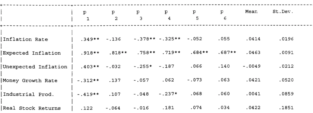
In Table 1 the autocorrelations of all the variables up to 6 lags are presented. The autocorrelations of the monthly returns to T-Bills are significant for all six lags, which suggests that the expectations about inflation measured by monthly nominal returns on T-bills are correlated with the previous month's rates. This can also be observed in most of the studies using US and other industrialized countries' data (See Fama and Schwert [8] and Mandelker and Tandon [15] ) . The autocorrelations of industrial production growth rates tends to decay zero after first lag. The money base growth rate data also have autocorrelations close to zero.
The real stock returns also have statistically insignificant autocorrelations in all 6 lags which should be the case when the inflation-related variation is eliminated.
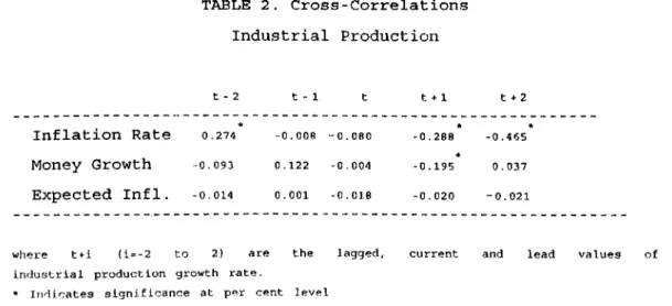
In Table 2, we present various cross-correlations. The money demand-quantity theory model predicts a negative correlation between inflation and real activity. Consistent with this hypothesis, the cross-correlations show that measures of current and future real activity have negative simple correlations both with actual inflation and with the expected inflation ratés, ev#=‘n
if the cross-correlations are statistically insignificant.
4. Results :
TABLE 2. Cross-Correlations Industrial Production t - 2 t - 1 t t -f 1 t + 2 Inflation Rate •k 0.274 -0.008 - 0.080 * -0.28B * -0.465 Money Growth ■'0.093 0.122 -0.004 *■ -0.195 0.037 Expected Infl. -0.014 0.001 -0.018 -0.020 -0.021
where t + i (i = -2 to 2) are the lagged, current and lead values of industrial production growth rate.
Indicates significance at per cent level
In Turkish case, however, although the money demand-quantity theory hypothesizes, we cannot observe a consistent positive relationship between money and real activity growth rates during the period of the study. This could be due to measurement problems and/or an inappropriate definition of money.
4.2. Inflation, Interest Rates, Money and Real Activity :
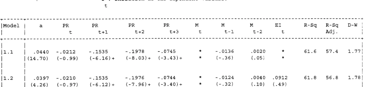
In Table 3A, estimates of the inflation derived from the money demand model (equations 1,1 and 1.2) are presented. In these regressions, the inflation rate, I^, is the dependent variable, while current and past money growth rates, current changes in interest rates (T-bill rates) and current and future levels of real activity are the independent variables.
Multicollinearity is a problem with models using multiple regressions with high number of lead and lag variables. However, the cross-correlations shown in Table 2 are small, only one of them is above 0.4. Thus, we can say that multicollinearity does not seem to effect the results significantly.
In the regression equation (1.2) we also include the expected inflation (T-bill rates) as an explanatory variable. In this regression, the coefficient of El is insignificant for a=0.05 significance level. The inclusion of El does not affect 2 significantly the coefficients of other variables. Also R improves only a. Therefore we can infer that the real activity variables have dominate the expected inflation in explaining the actual inflation. This is similar to Kama's [5] (1982) findings that interest rates have small explanatory power in inflation regressions.
The coefficients of past money growth rates on inflation have varying signs. Also they are statistically insignificant. The reason is that the money growth rates are autocorrelated (see App.A, D-W statistic is 1.16 which is less than 1.5). Also there
is the problem of Ml being a not-so-good measure of money.
When a whole range of lagged, lead and current values of money growth rates are used in the inflation regression, most of the coefficients have positive values (although insignificant). So we can infer (with caution) that inflation responds to money growth rates in a positive manner. The inflation regression including all past and future levels of money growth is given in A p p . A .
The results of the regression equations 1.1 and 1.^ indicate that there is negative relation between inflation and forecasts of real activity. We also observe a fairly high R^, %61 (adjusted R^ %57) . The residuals are tested for autocorrelation and no significant autocorrelation is detected. This result is consistent with the simple money demand-quantity theory in which "increases in anticipated real activity causes increases in real money 'V'manded, which are not completely satisfied by nominal money growth and hence are accommodated by opposite pric:<» movements."
TABLE 1. Autocorrelations of series of cata P 1 P 2 P 3 P 4 P 5 P 6 Mean St.Dev. 1 1 ¡Inflation Rate j .349** 1 1 - .136 - .378** - .325** - .052 .055 . 0414 .0196 ¡Expected Inflation .918** .818** .758** .719** .684** . 687** . 0463 .0091 ¡Unexpected Inflation .403** -.032 -.255* - .187 .066 .140 -.0049 . 0212 ¡Money G r o w t h Rate -.312** .13 7 - . 057 . 062 - .073 . 063 . 0421 . 0520 ¡Industrial Prod. -.419** .107 - . 048 - .237* .068 .060 .0041 .0859
¡Real Stock Returns . 122 -.064 - . 016 .181 .074 . 034 . 0422 .1851
p's are the autocorrelations at different lags * indicates significance at % 5 level
TABLE 3A. Regression Resnins
I : inflation as the dependent variable t -1-[ M o d e l 1 i ^
i
P R t P R t + 1 P R t + 2 P R t +3 M t M t - 1 M t -2 E l t R - S q R - S q A d j . D - W 1 1 1 -r 1 1 1 [ 1 . 1 1 1 . 0 4 4 0 - . 0 2 1 2 - . 1 5 3 5 - . 1 9 7 8 - . 0 7 4 5 * - . 0 1 3 6 . 0 0 2 0 * 6 1 . 6 5 7 . 4 i 1 . 7 7 1 1 1 1 ( 1 4 . 7 0 ) 1 1 ( - 0 . 9 9 ) ( - 6 . 1 6 ) + ( - 8 . 0 3 ) + ( - 3 . 4 3 ) + ★ ( - . 3 6 ) ( . 0 5 ) * 1i i 1 [ 1 . 2 1 1 . 0 3 9 7 - . 0 2 1 0 - . 1 5 3 5 - . 1 9 7 6 - . 0 7 4 4 ★ - . 0 1 2 4 . 0 0 4 0 . 0 9 1 2 6 1 . 8 5 6 . 8 1 1 . 7 8 j 1 ^ ---1 ( 4 . 2 6 ) ( - 0 . 9 7 ) ( - 6 . 1 2 ) + ( - 7 . 9 6 ) + ( - 3 . 4 0 ) + ★ ( - . 3 2 ) ( . 1 0 ) ( . 4 9 ) 111. * t values are in paranthesis
2. * values denote the variables w h ich are not included in the model 3. + indicates significance at 5 percent level
I : is the actual inflation rate
PR : is the real activity growth rate represented by industrial production
M : is the money base growth rate (includes currency in circulation plus demand deposits) El : is the expected inflation represented by T-bill rates
R : Real Stock Returns as the dependenc variable t
TABLii 3E. Regression Resulcs
Model 1 a 1 PR t PR t+1 PR t + 2 PR t+3 M t PR t-1 PR t-2 El t UEI t R-Sq R-Sq Adj . D-W 1 2.1 . 1780 * * ★ ★ * * ★ -3.998 -1.696 4.9 1.8 1.84 (1.45) * * * ★ ★ ★ * (-1.50) (-1.49) i 2.2 -.0096 * .357 .323 .198 ★ * ic * * 3.2 0.0 1.82 (-.41) * (1.22) (1.01) ( .68) ★ ★ ★ ★ ★ 2.3 -.0070 .3114 .4257 .1375 . 0594 * -.4951 - .3884 * * 11.9 2.1 1.80 (-.30) ( .95) (1.29) (.38) ( .19) * (-1.39) (-1.22) ★ ★ 2.4 . 1349 .2906 .4032 .1224 . 0548 * -.5109 -.4057 -3.065 * 14.4 3.1 1.87 (1.15) (.89) (1.23) (.34) (.27) * (-1.44) (-1.28) (-1.24) ★ 2.5 .1403 .2861 .4031 .1467 . 0976 -.1641 - .4886 - .4046 -3.037 * 14.6 1.4 1.88 (1.18) ( .87) (1.22) (.40) ( .28) (-.33) (-1.34) (-1.26) (-1.21) •k
1. * t values are in parenthesis
2. * values denote the variables which are not included in the model 3. + indicates significance at 5 percent level
I : is the actual inflation rate
PR : is th.e real activity growth rate represented by industrial production
M : is the m o n e y base growth rate (includes currency in circulation plus demand deposits) El : is the expected inflation represented by T-bill rates
4.3. Real Stock Returns, Real Activity, Inflation and Money :
In Table 3b, the results of stock return regressions on expected and unexpected inflation are presented. A negative relationship between real common stock returns and expected inflation as well as unexpected inflation can be observed, although they have coefficients not significantly different from
2
zero. So we can conclude, with caution, that this finding also verifies the results of other studies which rejects Fisher hypothesis that "common stocks, v/hich are claims to real assets, are hedges against inflation".
In the regression model of 2.2 the relationship between real stock returns and anticipations of real activity are presented. Although a positive relationship between two can be observed, the
2
coefficients are not significantly different from zero and and R is small. Although the coefficients are insignificant the Durbin-Watson statistic states that the results are not autocorrelated.
In model 2.4 we also incorporate expected inflation into the regression equation and find that the explanatory power of the equation increases slightly. The coefficient of expected inflation is not significantly different from zero and the coefficients of production growth rates do not seem to be effected much. Therefore, we can say that past real activity has more explanatory power than measures of inflation when both are used as independent variables for real stock returns.
As the last independent variable we add money growth rates in model 2.5 and find that adding this variable does not add much to the explanatory power of the equation. Money appears in a negative manner in the equation, but as stated above real
2
See Table 3B. Equat:ion 2.1
activity and expected inflation measures dominate money growth rates in explaining real stock returns.
As a conclusion of the tests of the real returns and real activity, insignificant positive relation between real stock returns and growth rates of future real activity is observed.
After examinig the real sector, we can say that, although the relationship between real stock returns and and real activity variables is not strong, there is a positive relationship between anticipations of real activity and stock returns. As we observed in the first set of regressions which examines the monetary sector, there is a strong negative relationship between inflation and anticipations of real activity. As a result of these conclusions we can say that the "proxy effect" hypothesis is also true for Turkish economy.
4.4. Assumptions and Limitations :
The basic assumptions made in this study are as follows
i) People make rational expectations and they have perfect foresight about real activity.
ii) Base money is assumed to be the currency-in-circulation plus demand deposits
iii) Monetary and real sectors of the economy are independent
iv) Short-term T-bill interest rates are good predictors of expected inflation.
A study of this kind also involves many problems and limitations. Some of these are ; price and interest rate controls over the period of study, problems of seasonality and causality, also the assumption of perfect foresight and fully rational expectations is a highly controversial issue.
rational expectations is a highly controversial issue.
The model also states that inflation and future real activity are negatively related. But whether the inflation rate adjusts to anticipations of future real activity or vice versa still remains an unresolved problem.
Another limitation is related with the data used. The industrial production growth rate was used to explain the relationship between stock returns and real activity. But most of the industrial companies in Türkiye do not have their common stocks traded openly in ISE. Which means the index of ISE may not reflect the real activity growth rate of whole economy, accurately.
5. Conclusion
The main hypothesis of this study is that the negative relationship between stock return and expected inflation can be explained by Fama's (1981,1982) "proxy effect" hypothesis which is derived from US stock market.
In this thesis I replicate Mandelker and Tandon [15]'s study for Türkiye, and follow Fama [5] and Fama and Gibbons [12], in testing the above relationship between stock returns, inflation and real variables.
A negative relationship between inflation and real activity
2
growth rates is found, and a fairly high is observed. This appears to be in contrast with prevailing belief that the inflation rate can be reduced by policies that discourage real activity. But we must also add that the interrelationships between inflation and real activity are much more complex then presented here. We also examine the coefficients of lagged growth rates of real activity variables, and find them to be more significant than those of future growth rates, (presented at App. A)
We also looked at the autocorrelations of the residuals of regressions models (1.1) and (1.2) and found no significant autocorrelation. Secondly, a first look at the regressions may indicate multicollinearity, but as shown in Table 2. the low cross-correlations among various variables do not indicate a serious problem.
The results state that, in the real sector, there is positive relationship between real stock returns and past growth rates of real activity variables. i.e.there is negative relationship between inflation and real activity growth rates. Tn
the real sector, we find a positive, although insignificant, relationship between real stock returns and past levels of real activity variables. We find that real activity dominates the money growth rates in explaining the real stock returns but it cannot dominate the expected inflation variable contrary to the findings of Fama [5].
The basic relationships given above, (1) the negative relationship between inflation and future real activity, and (2) the positive relationship between real stock returns and anticipated growth rates of real variables, can be combined to infer that there is negative relationship between stock returns and inflation.
Although there is a negative relationship between common stock returns and inflation, it is not strong enough to build up a trading strategy on it. The relationship between inflation and real activity is more sound and it is contrary to the commonly accepted view that an increase in the real activity will also increase the price level.
Finally, the role of money in Türkiye was not as strong as the role of money in US. The reason for this may be the high autocorrelation of monetary variables, or may be the definition of money base must be changed. Or the government policies on monetary growth may be reason of this result. Future research may concentrate on the relationship between money growth rates and real activity variables, also taking into account the monetary policies.
References :
1. J.Benderly and B.Zwick, "Inflation, Real Balances, Output, and Real Stock Returns," American Economic Review, Vol 75, No 5, Dec 1985, pp.1115-1123.
2. R.T.K.Cagli, "Common Stock Returns and Inflation :An Investigation of Fisher Effect for ISE," MBA Thesis-Bilkent University, Faculty of BA, Sept 1990.
3. R.A.Cohn and D.R.Lessard, "Are Markets Efficient? Tests of Alternative Hypothesis : The Effect of Inflation on Stock Prices
: International Evidence," Journal of Finance, Vol 36, No2, May 1981, pp.277-289.
4. E.Fama, "Interest Rates and Inflation : The Message In The Entrails, American Economic Review, Vol 67, No 3, June 1977, pp.487-496.
5. E.Fama, "Inflation, Output and Money," Journal of Business, April 1982, Vol 55, pp.201-231.
6. E.Fama, "Stock Returns, Real Activity, Inflation, and Money," American Economic Review, Vol 71, No4, Sept 1981, pp.545-565.
7. E.Fama, "Stock Returns, Real Activity, Inflation, and Money : Reply," American Economic Review, Vol 71, No4, Sept 1981, pp.471-472.
8. E.Fama and G.W.Schwert, "Asset Returns and Inflation," Journal of Financial Economics, 5, 1977, pp.115-146.
9. E.Fama and M.R.Gibbons, "A Comparison of Inflation Forecasts," Journal of Monetary Economics, 13, 1984, pp.327-348.
10. M.Feldsteiri; "Inflation and Stock Market," American Economic Review, Dec 1980, Vol 70, No 5, pp.839-847.
11. R.Geske and R.Roll, "The Fiscal and Monetary Linkage Between Stock Returns and Inflation," Journal of Finance, Vol 38, No 1, March 1983, pp.1-33.
12. N.B .Gultekin, "Stock Market Returns and Inflation : Evidence From Other Countries," Journal of Finance, Vol 38, No 1, March 1983, pp.49-65.
13. G.Kaul, "Stock Returns and Inflation : The Role of Monetary Sector," Journal of Financial Economics, 18, 1987, pp.253-276.
14. G.Kaul, "Monetary Regimes and The Relation Between Stock Returns and Inflationary Expectations," Journal of Financial and Quantitative Analysis, Vol 25, No 3, Sept 1990, pp.307-321.
15. G.Mandelker and T.Tandon, "Common Stock Returns, Real Activity, Money and Inflation : Some International Evidence," Journal of International Money and Finance, 1985, 4, pp.267-286.
16. F.Modigliani and R.Cohn, "Inflation, Rational Valuation and The Market," Financial Analysts Journal, 35, No 2, 1979, p p .24-44.
17. G.W.Schwert, "The Adjustment of Stock Prices To Information About Inflation," Journal of Finance, 36, 1, March 1981, pp.15-29.
18. B.Solnik, "The Relation Between Stock Prices and Inflationary Expectations : The International Evidence," Journal of Finance, Vol 38, No 1, March 1983, pp.35-48.
19. G.Soydemir, "The Linkage Between Stock Returns and Anticipated Inflation," Working Paper-Central Bank of Türkiye, Feb 1988.
20. A.Harwey, The Econome trie Analysis of Time Se.iies, LSF Handbooks in Economics, Philip Allan, 1990.
21. R .Ramanathan, Introductory Econometrics With Applirationr. Harcourt Brace Jovanovich Publishers, 1989.
A P P E N D I C E S
APPENDIX A
The statistical program MINITTVB's results are presented below
0.04 - O.OIMG 4- 0.12MG - 0.02MG + O.OIMG t - 6 t - 5 t : - 4 t - 3 + 0.07MG t-2 - O.llMGt- 1 + 0.02MGt 4 0.095MG t + 1 + - 0.07MG t»3 - O.IOMG t f 4 - 0.03MGt »-5 - 0.02 8MGt:+ 6
Predictor Coef Stdev t-ratio P
Constant 0.0399 0.0133 3.00 0.005 MG t: - 6 -0.0115 0.1174 -0.10 0.923 MG t: - 5 0.1228 0.1125 1.09 0.282 MG t: - 4 -0.0244 0.1175 -0.21 0.836 MG t - 3 0.0119 0.1185 0.10 0.920 MG t - 2 0.0717 0.1145 0.63 0.535 MG t - 1 -0.1109 0.1167 -0.95 0.348 MG t 0.0188 0.1232 0.15 0.879 MG t + 1 0.0947 0.1219 0.78 0.442 MG t + 2 0.0769 0.1179 0.65 0.518 MG t + 3 -0.0702 0.1198 -0.59 0.562 MG t + 4 -0.1024 0.1203 -0.85 0.400 MG t: + 5 -0.0273 0.1671 -0.16 0.871 MG t f6 -0.0275 0.1770 -0.16 0,877 s = 0.02233 R-sq = 10.2% R--sq(adj ) = 0.0% Durbin-Watson statistic = 1.16
APPENDIX B
The statistical program MINITAB's results are presented bel'^w
I = 0.043 + O.OlPR + O.OlPR + O.OlPR - 0.02PR
t - 6 t - 5 t - 4 t ^
- O.OlPR - 0.03PR - O.OlPR - 0.13PR - 0. V^PR
t - 2 t - 1 t t + 1
- 0.06PR + 0.05PR + 0.07PR - O.OlPR t + 3 t + 4 t + 5 t: + 6
Predictor Coef Stdev t-ratio P
Constant 0.0426 0.0028 15.30 0.000 PR t - 6 0.0053 0.0338 0.16 0.876 PR l: - 5 0.0093 0.0447 0.21 0.836 PR t - 4 0.0115 0.0454 0.25 0.801 PR t - 3 -0.0150 0.0477 -0.31 0.755 PR t - 2 -0.0104 0.0531 -0.20 0.846 PR l: - 1 -0.0269 0.0519 -0.52 0.608 PR t -0.0104 0.0503 -0.21 0.837 PR t + 1 -0.1287 0.0519 -2.48 0.017 PR t + 2 -0.1913 0.0526 -3.64 0.001 PR t f 3 -0.0593 0.0467 -1.27 0.211 PR t + 4 0.0510 0.0450 1.13 0.264 PR t + 5 0.0704 0.0444 1.59 0.121 PR t 4 6 -0.0054 0.0344 -0.16 0.876 s = 0.01215 R-sq = 73.4% R-sq(adj) r- 64.8 Durbin-Watson statistic = 1,65