B. Baygiin, F.
J.
Kuchuk, and O. Arikan
In this paper we describe a time domain algorithm for determining the influence function from the measured input and output signals of the system. The deconvolution, which is a highly unstable inverse problem with measurement errors, is an important step for obtaining the system's influence function that provides insight about flow regimes normally masked by the time-dependent input signal. The algorithms presented for deconvolution in the literature are generally based on data reduction, with the exception of constrained deconvolution methods.
We propose a constrained least-squares deconvolution method to reconstruct the influence func-tion from noisy data. The constraints are the lower bounds on the first few lags of the normalized autocorrelation coefficients of the influence function. The lower bounds may represent known or desirable smoothness properties of the function. By choosing the constraint values larger, a smoother deconvolution can be obtained. We also impose an energy constraint on the derivative of the recon-structed signal for further regularization.
Introduction
Deconvolution is a signal processing method in which the effect of the time-dependent input signal is extracted from the output signal. In testing, it is defined as deter-mining the influence function or unit response behavior of a system at the wellbore (the constant rate behav-ior) from measured downhole pressure and flow rate. 1 For convenience, this deconvolution is called
pressure-rate deconvolution. Recently, Goode etal.2 presented a different approach using pressure signals from the hor-izontal and vertical probes of the multi probe wireline formation tester3 to obtain the ratio impulse function of the system. The deconvolution method described by Goode et al.2 is called pressure-pressure deconvolution in this paper. The pressure-pressure deconvolution as shown in Appendix A can easily be extended to other >wll-testing problems, such as interference testing be-tween wells. For both methods, the deconvolution oper-ation can be defined as obtaining solutions for convolu-tion type linear Volterra integral equaconvolu-tions that can be written as
(1)
Copyright 1997, Society of Petroleum Engineers, Inc.
Paper first presented at the SPE Annual Technical Conference & Exhibition held in New Orleans. U.SA, 25-28 September 1995.
Received for review. August 19, 1996 Accepted for publication, January 23, 1997 Camera-ready copy received. March 31, 1997
SPE 28405
246
For convenience, we use p instead of /:lp. The kernel Q of the convolution integral is called the impulse re-sponse or the ratio of the impulse rere-sponses evaluated at two different locations (see Appendix A). Whether the kernel is an impulse resp onse or a ratio of impulse responses, the impulse response is a solution of the dif-fusivity equation for a Neumann-type internal boundary condition. As discussed by Kuchuk et al. 1 the deconvo-lution method given in this paper can also be applied to Dirichlet-type problems. The quantities p and
f
in Eq. 1 are measured as functions of time.The deconvolved kernel Q, and its integral (unit re-sponse) and logarithmic derivative forms (txQ ) are used in system identification, which is the first step of the >wll test interpretation. Many different deconvolution algorithms can be developed using different operational techniques. The most appropriate method for a partic-ular testing problem depends on the behavior and the noise characteristics of the measurements. In the ab-sence of noise, numerical algorithms for approximating the solution of Eq. 1 for the kernel Q \\QuId be rela-tively trivial. However, as discussed in Kuchuk et al., 1 even small amounts of noise in the flow rate have a detrimental effect on the solution. Consequently, Coats
etal.4 used a linear programming method with a num-ber of constraints in order to smooth the solution. An alternative constrained deconvolution method using lin-ear least-square minimization was presented by Kuchuk
et al.I The latter method gives a smooth solution for the integral of Q , but Q itself oscillates mildly. The oscilla-tory nature of the solution from the method of Kuchuk
et al. I sometimes hinders the identification step.
DECONVOLUTION UNDER NORMALIZED AUTOCORRELATION CONSTRAINTS In this paper, we propose a novel constrained
least-squares deconvolution method to r:econstruct the influ-ence function from noisy data. The constraints are the lower bounds on the first few lags of the normalized au-tocorrelation coefficients of the influence function. The lower bounds may represent known or desirable smooth-ness properties of the function. The inclusion of the au-tocorrelation constraints generates a regularization ef-fect on the deconvolution. Numerical results indicate that the proposed approach can significantly improve the quality of the deconvolution.
Formulation of the Problem
We first consider a discretized version of Eq. 1. We assume that the quantities p( t) and
J
(t) are measured at times to, tl, ... ,t N. It is desirable to find the values of9
at the same time points.An equivalent way of writing the convolution inte-gral in Eq. 1 is
p(t) =
lot
J(t - T)9(T)dT . (2)A discrete trapezoid approximation to the integral in Eq. 2 would be
n - l
p(tn)
=
L
J(tn - tk)9(tk)t.(k), 1 ::; n::; N, (3)k=O
where t.(k) is a scaling factor that is a function of the sampling interval lengths tk -tk-l and tk+l-tk (t-l
==
0). If the sampling times are uniformly spaced, i.e., the length of the sampling interval tk -tk-l is constant over
k, then the values J(tn -tk) correspond to the measured values of J(t), only in reverse order. On the other hand, if the sampling times are not uniformly spaced, then the time value (tn - tk) does not necessarily correspond to one of the original sampling times to, ...
,t
N. In the lat-ter case, the values J(tn - tk) should be approximated from the measured values J(to), ... ,J(tN). In our im-plementation, we compute the values J(t n - tk) using splines.Eq. 3 can be written using matrix notation as
y=Hx+w, (4)
where y is the observed output signal (pressure mea-surements) vector [P(t!), ... , p(t N )]T (the superscript T
denotes matrix transpose), H is a lower-triangular ma-trix representing the time variation of
J
(t) (the nth row ofH is [J(tn-tO)xt.(O), ... ,f(tn-tn_dxll(n-l)]),x is the signal vector [9(to), ... ,9(tN_d]T to be re-constructed (the desired deconvolution result), and w
(N xl) is the observation noise vector. We use bold-face lower and upper case characters to denote vectorial and matrix variables, respectively. w represents any discrepancy between the convolutional model and the actual observation y. We seek the vector x that best matches the observed y in the least-squares sense, i.e.,
min{lly - Hx112} .
x (5)
When there is no noise (w
==
0), the solution of the minimization problem in Eq. 5 can be found by premul-tiplying y by the inverse of the matrix H. Because His lower-triangular, the inverse exists unless some of the diagonal elements of H are zero. However, if the con-dition number (the ratio of the largest singular value of H to the smallest singular value) of H is high, the matrix inversion could be highly unstable, giving rise to an oscillatory deconvolution result. An alternative, but equivalent, recursive solution for x can be formu-lated exploiting the lower-triangular structure of H. In this solution, the elements of x are obtained starting with the first row and solving for Xl, then proceeding to the second row and solving for X2 , this time using the previously computed value of Xl, and then continuing down the rows of y and H. Unfortunately, this recur-sive solution fails with even the slightest noise on the right-hand side of Eq. 4, because the noise propagates over increasing indices of Xn. I Hence, in general, this recursive solution is not preferred.
To counter the adverse effects experienced in linear inversion, some sort of regularization is usually applied. Regularization can be affected by solving the minimiza-tion problem in Eq. 5 under a set of constraints. The deconvolution method we propose falls into this cate-gory. Basically, we suppress the effects of noise by im-posing smoothness constraints and the effects of an ill-conditioned H matrix by imposing an energy constraint.
Before we give a precise statement of the constraints, it is worthwhile to explain the reasoning behind them. By smoothness of the signal Xl, ... , X N represented by the vector x, we mean that the signal does not change rapidly. In other words, for any n, 1 ::; n ::; N - 1, we do not expect x(n) to be too different from x(n
+
1). Hence, if we compare the two vectors Zl~f[X2,X3,
. .. , xNfand
Z2~f[XI,X2'
.. . ,XN_IlT , they should be somewhat similar. The maximum similarity would be attained if Zl = z2, in which case Xl = X2 = ... = xN,i.e., if we have a constant signal. The minimum sim-ilarity would be attained if zl
=
-z2, in which caseXl
=
-X2=
X3= ... =
(-l)(N-1)xN. Clearly, in the latter case unless x==
0, we have a highly oscilla-tory signal, which is undesirable. The t'M) extreme cases suggest a mechanism to control the level of smoothness in x. First observe that due to the Cauchy-Schwarzinequality,S the following inequality always holds:
::;1
(6)Therefore, we can control the smoothness by imposing the following constraint:
"£;:~/
x(n)x(n+
1) (N
1
2)1/2(
N 2)1/2:::::B1 (7)"£n=l (x(n)) "£n=2(x(n))
and varying the value of B1 between -1 and 1. The higher the value of B1, the smoother the vector x.
Ha ving made this observation, we can generalize the smoothness constraints from adjacent samples x(n) and
x( n
+
1) to samples that are sufficiently close, i.e. x (n)and x (n
+
m), for 1 ::; m ::; M1 and 1 ::; n ::; N - m.More specifically, to impose similarity on samples that are m points apart, we can use the following constraint:
(8) where Bm ::; 1. Similarly to Eq. 6, one knows from the Camby-Schwarz inequality that the fraction in Eq. 8 is upper-bounded by 1. Therefore, higher values of Bm
give rise to greater similarity between samples that are m points apart.
In our applications, we found that for the purpose of obtaining the logarithmic derivative t x 9 (wehere
9
is usually the ratio of two impulse responses and t is time), it is better to impose smoothness constraints of the form given in Eq. 8 not on9
(i.e. on x) but ontxg. Furthermore, we made a slight modification on the
denominator. More specifically, we used the following set of constraints:
where
Xt~f[t(l)
x x(I), ... ,teN) x x(N)]T. In anal-ogy with the original development of a similar set of smoothness constraints in the context of stochastic sig-nal reconstruction in Ankan and Baygun,6 we refer to the constraints in Eq. 9 as "autocorrelation constraints." The constraints in Eq. 9 impose smoothness on the solution. To further reduce the problems associated with the inversion of an ill-conditioned matrix H, we use an energy constraint on the derivative d x of x:N
1)d
x(n))2::; Ct , (10) n=l 248 def T where dx=
[xt(2) - xt(I), . .. ,xt(N) - xt(N - 1)] .The formal statement of the proposed constrained deconvolution method, which combines the constraints in Eqs. 9 and 10, is as follows:
minimize x {Ily - Hx112} subject to: i.
"£;:
:l m x (n)x (n+
m)>
B "£~=l(x(n))2 - m, 1 ::;m::;
Ml N ii.l:)d
x(n))2::; Ct . n=lSolution of the Constrained Least Squares Problem (11)
(12)
(13)
The constrained least-squares problem in Eqs. 11 through 13 can be reformulated using the method of Lagrange multipliers. It can be shown that the cost function in Eq. 11 and the constraints in Eqs. 12 and 13 satisfy the required regularity assumptions so that the first order necessary conditions on the following Lagrangian func-tion characterize the constrained least-squares problem.
M
£(x,,X)
=
Ily - H xl12+
L
\ncm(x) , (14)m=l
where M
=
Ml+
1, ,X~f[A1'
... , AM]T is the vector of Lagrange multipliers, q, ... ,CM are the smoothness constraints on x, and C M is the energy constraint:em(x)
=
Bm"£;;=1
(t( n )x( n))2 - "£;;~rt(n)x(n)x(n +m)t(n +m) , l::;m::;M-l "£;:=1 (t(n+l)x(n+l) -t(n)x(n)f -Ct, m=M. (15) The first order necessary conditions (Kuhn-Tucker con-ditions) for optimality are as follows.\7x£(x,,X) =0
Am 2: 0, 1::; m ::; M
em(x) 2:0, l::;m::;M
Amem(X) = 0, 1::; m ::; M .
(16)
The first of these conditions provides a solution for x in terms of ,X . We show in Appendix B that this solution has the form
DECONVOLUTION UNDER NORMALIZED AUTOCORRELATION CONSTRAINTS where A is a matrix with entries that are functions of
A.
We can now write the dual of the original con-strained least-squares problem in Eqs. 11 through 13:
minimize
Ally -
H x(A)112 (18) subject to:Am
2:
0, 1:::;m:::;
M (19)Cm(X(A))
2:
0, 1:::;m:::;
M (20)AmCm(X(A))
=
0, 1:::;m:::;
M . (21)The dual problem has an important computational advantage over the original problem. While the original problem is an optimization over N variables Xl,·· . ,XN,
the dual problem is an optimization over M variables AI, ... ,AM, where typically M
«
N. For instance, in our numerical examples N is between 150 and 200, while M is 1 or 2.Results and Discussion
In this section, we apply our method to a few examples to demonstrate the improvement that can be achieved by using the constraints in the deconvolution. Let us suppose that we conduct a flow test with a dual-packer module of the multiprobe wireline formation tester (see Zimmerman et al.3 for more details about the tool) in a homogeneous formation. For this example, the input flow rate and the output packer interval pressure mea-surements are shown in Fig. 1. In addition to these surements, let us assume that the pressure is also mea-sured at 5 ft above from the center of the packer module with an observation probe. Figure 1 also presents the observation probe measurements. The distance between the packers (the length of the open interval) is 3.2 ft with a well radius of 0.35 ft. The formation and fluid prop-erties for the example are kh
=
100 md, kv=
10 md,h = 10 ft, Zw
=
5 ft (the vertical distance from the cen-ter of the open incen-terval to the bottom of the formation), ¢=
0.20, fl= 1
cp, and Ct=
1.0 xlO-5 psi-I.As described in Appendix A, let us obtain the 9 function for this formation from the pressure-pressure deconvolution of the pressure measuremen ts at both packer and observation probes. To achieve acceptable com-putation speed, we limit the number of constraints to M :::; 2. In other words, we consider a smoothness con-straint only on consecutive samples and/or the deriva-tive energy constraint. We present both noiseless and noisy examples. The data are synthetic data and the noise is assumed to be uniformly distributed within a specified band about the true convolution result Hx. The result of the deconvolution is denoted by
x.
We start with the noiseless case to emphasize that although the inverse of the H matrix exists theoreti-cally, there may be computational problems in practice.
·01 a. 80 ~6D
~
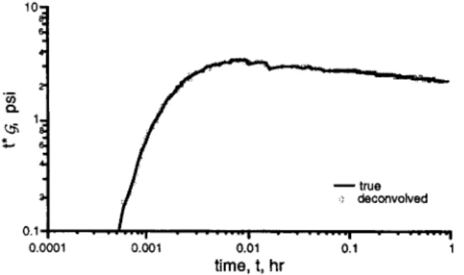
CD "fi 40 ! ffi ~ 0.20 0.0001 0.001 0.01 time,t, hr 0.1Fig. 1-Flow rate and packer and probe pressures. The result of the direct inversion, which was extremely poor, is not shown here. In Fig. 2, we present the decon-volution result under the derivative energy constraint. As can be seen, the deconvolution result
x
matches the true x very closely. We have also obtained ~ry similar results with only the autocorrelation constraint.We noted previously that the recursive computa-tion method gives a reliable deconvolucomputa-tion result in the noiseless case. However, because the recursive method suffers heavily with the addition of even a little noise, that method will not be considered in our examples.
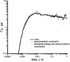
Next, ~ look at the noisy case. The result for
1%
additive noise using the autocorrelation constraint only is given in Fig. 3. Note that the general trend of x is captured in the deconvolution result
x.
The oscilla-tions towards the end can be suppressed by adding the energy constraint on the derivative. Fig. 3 also shows the result with both derivative energy and autocorrela-tion constraints. The late-time oscillaautocorrela-tions inx
are now lower than before and the deconvolution result matches the original signal x more closely.-true ) deconvolved 0.1-+--__ .... ...y'-... ..,... _ _ . _ ... . . . , . . - - _ ... 0.0001 0.001 0.01 time, t, hr 0.1
Fig. 2-True and deconvolved
tx
(j
under the derivative energy constraint in the noiseless case.'iii Co
10
-true
autocorrelation constraint derivative energy and autocorrelation
constraints
0.1 +-r..,...,-+n-nr-... ..,...,TTl1T"""'"T..,...,,.,.,.,mr""'"T-rrrTlIII
0.0001 0.001 0.01 time, t, hr
0.1
Fig. 3-True and deconvolved
tx
(j
using the autocorrelation constraint and both derivative energy and autocorrelation constraints with 1% additive noise.Figs. 4 shows the deconvolution results for 2% ad-ditive noise under each of the constraints separately as well as under both constraints. Fig. 4 shows that using only the autocorrelation constraints we get a good fit at early-time, while at late-time, we have oscillations. The important point is that the solution oscillates about the true x. In other words, the solution does not have a bias. If we use the derivative energy constraint instead of the autocorrelation constraint, then, as Fig. 4 shows, the late-time oscillations become lower but at the ex-pense of a mismatch at early-time. The deconvolution result can be improved by using the two constraints to-gether, which gives us the solution depicted in Fig. 4. Simultaneous use of the two constraints provides a good fit at early-time and ensures a low level of oscillation at late-time.
10
.~
_true
autocorrelation constraint
1 derivative energy constraint
.. derivatiVe energy and autocorrelation constraints
0.1+-_ ... - r _ _ ... - ... r-... ...,
0.0001 0.001 0.01 0.1
time, t, hr
Fig. 4-True and deconvolved
tx
(j
using the autocorrelation constraint and both derivative energy and autocorrelation constraints with 2% additive noise.250
In Fig. 5 we provide the results for a high noise case, where 5% noise was added to the convolution re-sult and both energy and smoothness constraints were used. Even with significant noise, the deconmlution re-sult shown here follows the true x reasonably closely. The conclusion from this and previous examples is that when both autocorrelation and energy constraints are used, the deconvolution is quite smooth and approxi-mates the true x closely, even with significant measure-ment errors.
10
_true
derivative energy and autocorrelation constraints
O.l+"""T-rrlt."."r--"T"'T'TTTI'II'T'-... ..,..., ... rr-... ..,...rT'ITm
0.0001 0.001 0.01 time, t, hr
0.1
Fig. 5-True and deconvolved
t
X(j
using both derivative energy and autocorrelation constraints with 5% additive noise.Conclusions
In this paper we present a novel time-domain algorithm for extracting the influence function from the measured input and output signals of a system. We pose the prob-lem in a least-squares minimization framework. The novel aspect of our approach is a set of constraints that provides a regularization to the ordinary least squares solution. We consider two different constraints: auto-correlation constraints and derivative energy constraints. We present numerical examples which demonstrate that, at late-time, our deconvolution result oscillates about the true influence function, i.e., our result does not have a bias away from the true solution. Furthermore, the magnitude of the late-time oscillations, which can be high in deconvolution results obtained by other meth-ods, are suppressed significantly by our method. There-fore, the deconvolution result describes the true influ-ence function \{)ry closely.
Nomenclature
A defined by Equation B-2
c compressibility, psi-1 [Pa-1 J or constraint
DECONVOLUTION UNDER NORMALIZED AUTOCORRELATION CONSTRAINTS d derivative D defined by Equation B-7 G Green's function 9 impulse response h thickness, ft [m] k permeability, md [m2] p pressure, psi [Pal
q flow rate, RB/D [m3s-1 ]
r radius or position vector, ft [m] s Laplace transform variable
t time, hours [s]
a bound on derivative energy A Lagrange multiplier
J.L viscosity, cp [pas]
4> porosity, fraction
r dummy integration variable
e
bound on autocorrelationy defined by Equation B-3 C Lagrangian
g
a ratio of impulse responses V' gradient Subscripts h horizontal m measured or m - th 0 initial or original t total v verticalw well or well bore
x x with respect to x with respect to x
Superscripts
T transpose
= estimate (deconvolution result) Acknowledgments
We are grateful to Schlumberger for permission to pub-lish this paper.
References
1. Kuchuk, F. J., Carter, R. G. and Ayestaran, L.: "Deconvolution of Well bore Pressure and Flow Rate,"
SPEFE (1990) 53-59.
2. Goode, P. A., Pop, J. J., and Murphy lIT, W. F.: "Multiple Probe Formation Testing and Vertical Reservoir Continuity," SPE 22738 presented at the SPE Annual Technical Conference and Exhibition, Dallas (Oct. 1991).
3. Zimmerman, T., MacInnis, J., Hoppe, J., Pop, J. and Long, T.: "Application of emerging wireline formation tester technologies," OSEA-90081, Eighth Offshore Southeast Conf. (Dec.), Singapore (1990). 4. Coats, K. H., Rapoport, L. A., McCord, J. R., and
Drews, W. P : "Determination of Aquifer
Influ-ence FUnctions From Field Data," JPT (Dec. 1964) 1417-24.
5. Luenberger, D. G: Optimization by Vector Space
Methods, Wiley, New York (1969).
6. Ankan, O. and Baygiin, B.: "Least-Squares Sig-nal Reconstruction Under Normalized Autocorre-lation Constraints," Proceedings of ICASSP-94, Adelaide, Australia (April 1994).
Appendix A: Pressure-Pressure Deconvoptlution Let us consider pressure diffusion in a three-dimensional infinite (unbounded) porous medium for a flow of a slightly compressible single-phase fluid with pressure and time-invariant fluid and formation properties. The pres-sure distribution in a such system due to a prescribed fluid flux (a Neumann-type boundary condition which is the flow rate for our problem) at an internal boundary surface can be written as
p(t,r) =po
-l~o-
drqm(r)g(t -r,r) ,
(A - 1)where po is the initial pressure,
r
is the spatial position vector, and t is the time. In Eq. A-I, the flow rate (pre-scribed fluid flux) qm and the impulse response 9 are zero for t<
O. The expression given by Eq. A-I is known as Duhamel's theorem. The impulse response 9 is a so-lution of the diffusivity equation for a Neumann-type internal boundary condition. The pressure distribution given by Eq. A-I can easily be generalized for multiple internal boundary surfaces in unbounded or bounded systems.Clearly, the pressure-rate deconvolution is nothing more than obtaining 9 in Eq. A-I from the measured p
at a given r (at any point in the spatial domain) and
qm measured at the internal boundary. Let us write the Laplace transform of Eq. A-I at two different spatial locations rl and r2 as
6p(s, n)
=
tim(S)g(S, n) (A - 2)and
6])(s,r:z) =tim(S)g(s,r2) , (A - 3) where 6p = Po - p(t, r). As described by Goode et al.,2
solving Eq. A-2 for tim and substituting it in Eq. A-3, we obtain the Laplace transform of the pressure at r2 as
6]5(s, r2) = 6p(s, rdQ(s) , (A - 4)
where Q (s)
=
~iS.r2l
that is calledg
function. 2 In the 9 S,rttime domain, Eq. A-4 can be written as
Obtaining
9
in Eq. A-5 from measured ~p(t, q)
and ~p(t,1'2)
is called pressure-pressure deconvolution.For an interference test, ~p(t, rl) can be the pres-sure at the pulse well, while ~p(t, r2) can be the pres-sure at the observation well. For a vertical interfer-ence test within the wellbore, ~p(t, n) can be the pres-sure at the pulse (injection or production) interval while
~p(t, r2) can be the pressure at the observation interval. For this test configuration, the pulse interval is normally isolated from the observation interval by a packer. For the multi probe wireline formation tester, ~p(
t,
n) can be the pressure at the sink probe or the horizontal probe, while ~p(t, r2) can be the pressure at the observation probe.Appendix B: Solution of the First Kuhn-Tucker Equation
The smoothness constraints em (x), m = 1, ... ,M - 1 in Eq. 15 can be written as
em(x) =
BmxT (yTy)
x -xTyT AmY
x, (B - 1) whereAm
~f [~
INom]
(B - 2)~~f
['T:
t(U
(B - 3)and IN _ m is the identity matrix of order (N - m).
Now note that for any N -vector z the following identity holds.
T I T (
T)
Z Amz =
iZ
Am+
Am z .. (B - 4) Therefore, taking Z = Y x for 1:s:
m:s:
M - 1 we obtainem(x) =
BmxT (yTy)
x -}xTyT
(Am
+ A!n ) y
x=
xT yT [BmI
~
-
~
(
Am+A!n)]Yx.
(B - 5) Similarly, the final constraint CM(X)
=
dI dx - 0:can be written a (B - 6) where 252 [ -1
D~f
!
1 0 -1 1 0o
-1 (B - 7)is the (N - 1) x N derivative matrix. Using Eqs. B-5 and B-6 we can rewrite the Lagrangian function £( x,
oX)
defined by Eq. 14 as follows:Now let
(B - 9)
By using the A matrix, we can express the Lagrangian function in Eq. B-8 as
This leads to the following expression for the partial gradient of the Lagrangian function with respect to x:
(B - 11) Equating this expression to zero gives the desired solu-tion of x as
SI Metric Conversion Factors cp
x
1.0*ft
x
3.048* mdx
9.869223psi x 6.894757 *Conversion factor is exact
E-03
=
Pa. s E-Ol =m E-04 = J.1m2 E+OO =kPa (B - 12) SPEJ BOient Baygiin is currently with Salomon Brothers Inc., working as an analyst in the Fixed Income Research Division, 7 World Trade Center, New York, New York 10048, email: [email protected] to joining Salomon Brothers, he worked for Schlumberger-Doll Research, from 1992 to 1996. He received BS and MS degrees in electrical engineering from the Middle East Technical University,Ankara, Turkey, in 1986 and 1988, respectively. He
received an MS degree in mathematics in 1991 and a Ph.D.
DECONVOLUTION UNDER NORMALIZED AUTOCORRELATION CONSTRAINTS degree in electrical engineering in 1992, both from The
University of Michigan.
Fikri J. Kuchuk is Chief Reservoir Engineer for Schlumberger Middle East, Schlumberger Technical Services, 8th Floor, Dubai International Trade Center, P. O. Box 9261, Dubai, United Arab Emirates, email: [email protected]. He was a senior scientist and a program leader at Schiumberger-Doll Research Center, Ridgefield, Connecticut, USA. He was a consulting professor in the Petroleum Engineering Department of Stanford University from 1988 to 1994. Before joining Schlumberger in 1982, he worked for Sohio Petroleum Company. He holds an MS degree from the Technical University of Istanbul, and MS and Ph.D. degrees from Stanford University, all in petroleum engineering.
Orhan Arikan is Assistant Professor of Electrical and Electronics Engineering at Bilkent University, Ankara, Turkey, email: [email protected]. His current research interests are in adaptive signal processing, and time-frequency signal analysis. Before joining Bilkent University, he worked for three years as a Research Scientist at Schiumberger-Doll Research, Ridgefield, Connecticut, USA. He holds a B.Sc. Degree in Electrical Engineering from the Middle East Technical University and MS and Ph.D. degrees both in Electrical and Computer Engineering from the University of Illinois at Urbana-Champaign.