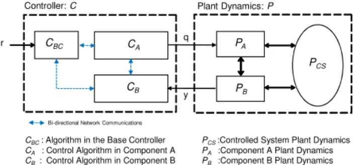
Combined component swapping modularity for a VCT engine controller

Genel olarak bakıldığında Güzel Sanatlar Bölümü Resim-İş Eğitimi ABD ve Müzik Eğitimi ABD’nda okuyan öğrencilerinin %15,2’si yani 26 öğrenci bireysel

Summing up a short review of the national movement of the Soviet Turks under the conditions of the modern ethnic processes in the USSR and taking into account the fact that

A vrupa Üniversiteler Birli¤i (EUA) taraf›ndan haz›rla- nan Global University Rankings and Their Impact (Küresel Üniversite S›ralamalar› ve Etkileri) bafll›kl›

1) Morfo-fizyolojik özellikler bakımından genotipler arasında önemli düzeyde farklılıklar bulunmuĢtur. Determinat tipler, indeterminat tiplere oranla daha

Deve lopm ent Process: Diagn osing the Syste m and its Probl ems... Ömer DİNÇER (işletme Yönetim i Bilim

Çalışanlar tarafından haber uçurma (whistleblowing) iki şekilde yapılmaktadır; içsel whistleblowing (internal whistleblowing), haber uçuranın örgüt içindeki ahlaki

CONTROLLER DESIGN To control the system given by equations 2–10 we propose a novel control law, which consists of a dominant controller and a parallel controller to ensure

Testing of data is done to test whether the training phase has been successful or not the testing data is used to test the data after the training this ensure that the prediction