Application of asymptotic waveform evaluation for time-domain analysis of nonlinear circuits

Application of asymptotic waveform evaluation for time-domain analysis

of nonlinear circuits

SATILMIS

¸

TOPCËU² , ABDULLAH ATALAR³ and MEHMET A. TAN³

A method is described to exploit asymptotic waveform evaluation (AWE) in the time-domain analysis of nonlinear circuits by using SPICE models for nonlinear devices such as diodes, transistors, etc. Although AWE has been used for linearized circuits only, the aim is to enhance the accuracy of the simulation while preserving the computational e ciency obtained with AWE and to eliminate the piecewise-linear modelling problem. Practical examples are given to illustrate signi® cant improvements in accuracy. For circuits containing weakly nonlinear devices, it is demonstrated that this method is typically at least one order of magnitude faster than SPICE.

1. Introduction

Asymptotic waveform evaluation (AWE

)

(Pillage 1990

)

is a recent technique which is e€ ective in the time-domain analysis of linear(ized

)

circuits (Huang 1990

)

. It accurately produces a reduced-order model of the time-domain response of a linear circuit in terms of few dominant complex poles and residues. After it being developed by Pillage (1990

)

, AWE has been applied to many CAD problems. A survey of all these studies and the evolution of AWE is presented by Raghavan (1993

)

.

AWE is typically two or three orders of magnitude faster than traditional simu-lators in analysing large circuits. However, it can handle only linear(ized

)

circuits, whereas the time domain analysis problem is generally nonlinear due to the presence of nonlinear devices such as diodes and transistors in VLSI circuits. Previous attempts to apply AWE to the transient analysis of nonlinear circuits (Dikmen 1991, Kao 1992

)

solved this problem by using piecewise-linear (PWL

)

models for nonlinear elements. Although there exist programs that provide PWL models for given analytical expressions, it is di cult to ® nd a good PWL model that ® ts well to the actual i± v characteristics of a nonlinear device. The problem is that if the PWL model consists of a few segments, this reduces the accuracy level of the simulation results; but if the PWL model is formed with too many segments, this time the user su€ ers from very long simulation times. The method presented in this paper uses SPICE models for nonlinear elements in the circuit. Hence, there is no modelling problem and we can obtain very accurate results which can be useful, for instance, in evaluating the critical path in a given circuit. In addition to this, we can adjust the

0020± 7217/97 $12.00Ñ 1997 Taylor & Francis Ltd.

Received 22 November 1996; accepted 13 January 1997.

² Department of Electrical and Electronic Engineering, Eastern Mediterranean University, GazimagÆusa, via Mersin 10, Turkey. Fax: +90 392 3669240; e-mail: topcu@eenet.ee.emu. edu.tr.

³ Electrical and Electronics Engineering Department, Bilkent University, 06533 Bilkent, Ankara, Turkey.

accuracy level by varying some parameters. If the required level of accuracy is increased, more simulation time is needed, as expected.

We describe the method and explain the extraction of linear equivalents of non-linear elements using SPICE models in§2. In §3 some examples are provided to illustrate the e ciency and accuracy of our method compared with the SPICE performance. Finally, our concluding remarks are given in§4.

2. The method

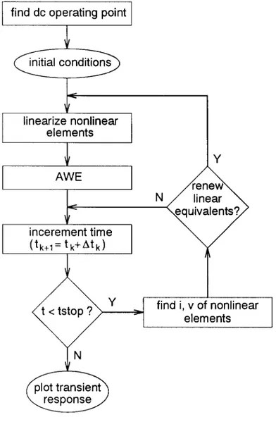
Our method is a new approach using the AWE technique to ® nd the time-domain response of nonlinear circuits containing diodes, transistors, etc. With the given SPICE models, our method can extract a linear equivalent for each nonlinear ele-ment about its bias point. For each nonlinear eleele-ment, it can also calculate the error caused by the linear equivalent while the operating point moves to any arbitrary direction. We have an easily calculated error criterion used for this purpose. When the error of any nonlinear device exceeds a user-speci® ed threshold at any time, the new linear equivalents are produced for all nonlinear elements about their present operating points. The steps of our method, for which a ¯ owchart is given in Fig. 1, can be outlined as follows.

(a

)

Find the DC operating point of the circuit by using the Newton± Raphson iteration (Vlach 1983

)

. This step is the ® rst nonlinear DC analysis which gives the initial conditions.

(b

)

Obtain linearized equivalents for all nonlinear elements in the circuit. For a diode, this step is simply replacing the diode by a Norton equivalent which represents the tangent approximation to its i± v curve about the presumed operating point.

(c

)

Perform an AWE to ® nd the time-domain behaviour of energy storage ele-ments in the circuit.

(d

)

Increment the time by the internal time step: tk+1=tk+ D tk. If the end time of the simulation is reached, then stop. Otherwise, continue with the next step.

(e

)

Solve the linear circuit equations to ® nd the branch currents and branch voltages of nonlinear elements. Compute the error due to linear equivalents of individual nonlinear elements. If at least one of them has an error greater than a user-speci® ed threshold value, then go to the step (b

)

. Otherwise, go to step (d

)

.

2.1. L inearization of an MOS transistor

In general, a nonlinear circuit may contain various types of transistors. Without loss of generality, we can concentrate on the MOS transistors. For simplicity, we have used the Level 1 MOSFET model of the SPICE (HSPICE 1992

)

which repre-sents the basic device characteristics, including the body e€ ect and the channel length modulation (Divekar 1988

)

. The DC drain-to-source current idsin the Level 1 MOS model is determined as follows.

Cuto€ region: vgs

£

vt

Linear region: 0

<

vds

<

vgs

-

vt ids=b

(

1+ L AMBDA

´

vds

)

(

vgs

-

vt

-

v₂ds

)

vds

(

2

)

Saturation region: 0

<

vgs

-

vt

£

vds ids=b 2

(

1+ L AMBDA

´

vds

)

(

vgs

-

vt

)

2

₍

3

)

where b = KP W L

( )

(

4

)

The threshold voltage is calculated as follows: vt=

V TO+ GAMMA

(

Ï

PHIê ê ê ê ê ê ê ê ê ê ê ê ê ê ê ê ê ê ê ê ê+vsb

-

Ï ê ê ê ê ê ê ê ê êêPHI

)

,

if vsb

³

0 V TO+ GAMMA 0.5 vsb ê ê ê ê ê ê ê ê êê PHI Ï

(

)

,

if vsb

<

0

ì

ï

í

ï

î

(

5

)

where L AMBDA, KP, V TO, GAMMA and PHI are the SPICE MOS model para-meters (HSPICE 1992

)

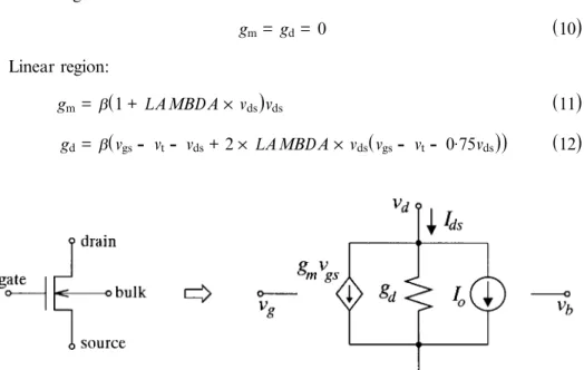
. The parameters W and L represent the width and length of an MOS transistor, respectively.

The linear DC equivalent circuit of an n-type MOSFET is given in Fig. 2. As may be seen, the transistor is modelled by a voltage controlled current source shunted by a conductance and a constant current source. In this linearized model, the drain-to-source current is calculated as follows:

Ids=gmvgs+gdvds+I0

(

6

)

where gm=

_¶

¶

₍

(

i_vds

)

gs

)

(

7

)

gd=

_¶

¶

₍

(

_vids

)

ds

)

(

8

)

I0= ids

-

gmvgs

-

gdvds

(

9

)

The partial derivatives gmand gdare called the transconductance and conductance, respectively, and they are calculated in each operating region of the transistor as follows. Cuto€ region: gm= gd= 0

(

10

)

Linear region: gm=b

(

1+ L AMBDA

´

vds

)

vds

(

11

)

gd=b

(

vgs

-

vt

-

vds+2

´

L AMBDA

´

vds

(

vgs

-

vt

-

0.75vds

))

(

12

)

Saturation region:

gm= b

(

1+ L AMBDA

´

vds

)

(

vgs

-

vt

)

(

13

)

gd= b

2L AMBDA

(

vgs

-

vt

)

2

₍

₁₄

₎

2.2. Deciding to renew the linear equivalents of nonlinear elements

As seen in Fig. 1, after incrementing the time we must decide about whether the linear equivalents of nonlinear elements will be renewed or not. This decision is made by ® nding the di€ erence between the actual i± v characteristics of the device and the operating point calculated by using the linear equivalent. If this di€ erence is greater than a user-de® ned threshold value, than the new linear equivalents are created for all nonlinear elements. For an MOS transistor, the di€ erence mentioned above is equal to

d i=

|

ids

-

Ids

|

(

15

)

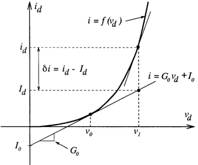
where ids and Ids are the drain-to-source current values calculated from the SPICE Level 1 MOS model and the linear equivalent, respectively, using the branch voltages vgsand vds. Calculation of the di€ erence in the case of a diode is shown in Fig. 3. As seen in Fig. 3, the diode has been linearized about vd=v0 and it is replaced by the Norton equivalent which consists of a current source of value I0 shunted by a conductance G0. In this case, when the diode branch voltage vd becomes equal to

v1, the di€ erence between the linear segment and the nonlinear i± v characteristics is

d i=id

-

Id. If the value of d i is greater than a user-speci® ed error tolerance limit,

than a new linearization must be made for the diode at vd= v1. Note that, to ® nd the error caused by the linear equivalents, we use the di€ erence between current values

instead of voltage values. Calculation of the di€ erence in current values requires less computation than the calculation of the di€ erence in voltage values, especially for three-terminal elements such as MOS transistors, because we concentrate on the voltage-controlled devices without loss of generality.

3. Results

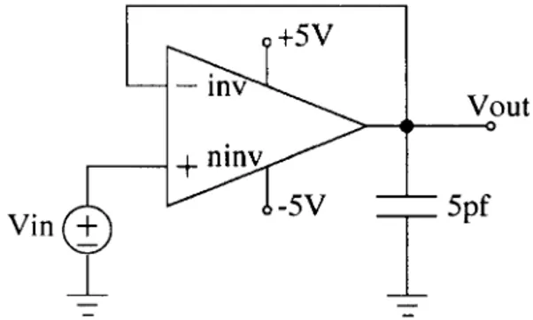
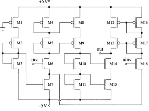
To illustrate the accuracy performance of our method, we have chosen some example circuits. The ® rst example is an opamp circuit with unity gain feedback, shown in Fig. 4. The schematic of the opamp (Gray 1983

)

is given in Fig. 5. The capacitors from each node to ground are not shown in Fig. 5, for clarity. We have used a pulse of small amplitude for the input voltage.

We have simulated this example circuit by using our method, HSPICE (HSPICE 1992

)

and SPICE3 (Quarles 1989

)

with di€ erent error thresholds. First of all, a reference result that is assumed to be very accurate is obtained by means of HSPICE using very tight error tolerance parameters and a very small internal time step. Then we have assumed this result to be the exact response of the circuit and all other simulation outputs are compared with this result to estimate their accuracy. The error in a simulation output is calculated by ® nding the average of absolute di€ erences with respect to the exact response at every timepoints where the output waveforms are printed. That is

average absolute difference= 1

N

å

N k=1

|

vexact

(

tk

)

-

vc

(

tk

)

|

(

16

)

where vexact

(

t

)

and vc

(

t

)

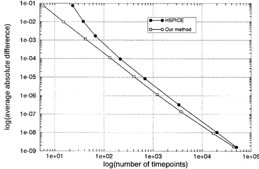
are the exact and calculated responses of the circuit, respec-tively. For all simulations, N is chosen as 1000. The accuracy versus number of timepoints for our method, HSPICE and SPICE3 is plotted in Fig. 6 for the opamp circuit. Here, the horizontal axis denotes the number of timepoints that a simulator needs to take to preserve the corresponding accuracy. At each timepoint HSPICE or SPICE3 performs a Newton± Raphson iteration whereas our method performs, in addition to Newton± Raphson, an AWE which costs one LU-decom-position and a few forward-backward substitutions (FBSs

)

. This means that, for a single timepoint, our method spends approximately twice as many CPU seconds than HSPICE or SPICE3. It is assumed that one FBS takes negligible CPU time compared to the time taken by one LU-decomposition for large circuits.

It is observed from Fig. 6 that HSPICE and SPICE3 have the same accuracy versus speed graphs because both of them are using a trapezoidal integration algo-rithm in the transient analysis. It is seen that our method can produce transient responses which are accurate up to nine signi® cant digits and it requires approxi-mately 1

20 of the number of timepoints needed by HSPICE to provide the same

Figure 6. Accuracy comparison between our method and SPICE for the opamp circuit. Figure 5. Schematic of the operational ampli® er at transistor level.

F ig ur e 7. R C tr ee dr iv en by a C M O S in ve rt er an d th e in pu t vo lt ag e fu nc ti on .

accuracy. If the user agrees to obtain less accurate results, such as having an error about 10-4, this ratio becomes 1

30. Then our method becomes approximately 15 times faster than HSPICE or SPICE3.

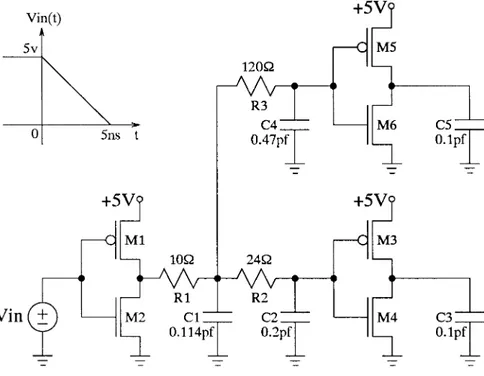
Our second example, given in Fig. 7, is a small RC tree driven by a CMOS inverter. This circuit is chosen as an example to explore the e€ ect of inserting non-linear elements into a non-linear circuit for which AWE provides very accurate results e ciently. Again, by using HSPICE we have obtained a reference result which is assumed to be extremely close to the exact result. Then we have simulated the example circuit using our method and HSPICE by changing the error tolerance parameters. These simulation results are compared with the reference result to esti-mate their accuracy levels. We have plotted the graph in Fig. 8 which shows the accuracy versus number of timepoints required by each simulator. It is observed from Fig. 8 that if the desired accuracy is low, our method is several times faster than HSPICE. However, when the accuracy is increased, both simulators need approximately the same number of timepoints.

In the third example, shown in Fig. 9, we have inserted additional MOS transistors into the second example to increase the number of nonlinear elements in the circuit. In a similar way to the previous example, we have obtained the graph of accuracy versus number of timepoints required by our simulator and HSPICE. The resultant graph is shown in Fig. 10. It can be observed from Fig. 8 and Fig. 10 that increasing the number of nonlinear elements inserted into a linear circuit causes a degradation in the speed performance of our method. Because the overall nonlinearity of the circuit is increased by additional MOS transistors, we need to renew the linear equivalents for the nonlinear elements more frequently as time goes on.

Figure 8. Accuracy versus speed graphs for our simulator and HSPICE in the second example.

Figure 10. Accuracy versus speed graphs for our simulator and HSPICE in the third example.

4. Conclusions

A new method is proposed to apply the AWE technique to the time-domain analysis of nonlinear circuits. The existing approaches which addressed this problem have utilized the PWL modelling for nonlinear elements. However, those methods have two major drawbacks: Finding good PWL models for nonlinear elements is a di cult problem; and PWL approximation results in low accuracy in time-domain responses. Our method overcomes these disadvantages by using the SPICE models for nonlinear elements. In our method, by means of error tolerance parameters the accuracy level of the simulation can be adjusted by the user. The software implementation of the method is very easy. We have presented some examples to show the e ciency and the accuracy performance of the method and to compare them with those of SPICE. The method is capable of providing an accuracy of 10-9 which cannot be obtained by the PWL modelling approach.

It is observed from the examples that our method is of advantage in situations when weak nonlinear circuits are studied. However, just for those cases, PWL AWE is also possible but our method is considerably superior to PWL AWE in terms of accuracy. As the nonlinearity of a circuit is increased by inserting additional non-linear elements, the e ciency of the method begins to decrease. That is, it will work for mild nonlinearities where the accuracy of SPICE is dictated by local truncation error of trapezoidal integration algorithm. Unfortunately, we can say that for large circuits with many nonlinear elements it may take more CPU time than taken by HSPICE to preserve the same accuracy level.

ACKNOWLEDGMENT

HSPICE is a trademark of Meta-Software Inc. References

Dikmen, C.T., 1991, Piecewise linear asymptotic waveform evaluation for transient simulation of electronic circuits. Proceedings of the IEEE International Symposium on Circuits and

Systems, pp. 854± 857.

Div ek a r, D. A., 1988, FET Modeling for Circuit Simulation (Boston, Massachusetts, U.S.A.:

Kluwer Academic).

Gr ay, P. R., 1983, Analysis and Design of Analog Integrated Circuits (Wiley).

HSPICE User’s Manual, 1992 (Campbell, U.S.A.: Meta-Software Inc.).

Huang, X., 1990, AWEsim: a program for the e cient analysis of linear(ized)circuits. IEEE

International Conference on Computer-aided Design, Technical Digest, pp. 534± 537.

Kao, R., 1992, Piecewise linear models for switch-level simulation. Technical Report # CSL-TR-92-532, Stanford University, Stanford, California, U.S.A.

Pillag e, L.T., 1990, Asymptotic waveform evaluation for timing analysis. IEEE Transactions

on Computer-aided Design,9, 352± 366.

Qua rles,T. L., 1989, Spice3 version 3c1 User’s Guide. Memorandum No. UCB/ERL M89/46, University of California, Berkeley, California, U.S.A.

Raghavan, V., 1993, AWE-Inspired. Proceedings of the IEEE Custom Integrated Circuits

Conference, pp. 18.1.1± 18.1.8.

Vlach, J., 1983, Computer Methods for Circuit Analysis and Design (New York: U.S.A.: Van Nostrand Reinhold).