Uluslararası Mühendislik Araştırma ve Geliştirme
Dergisi
International Journal of Engineering Research and
Development
Cilt/Volume:9 Sayı/Issue:3 Aralık/December 2017 https://doi.org/10.29137/umagd.372979
Araştırma Makalesi / Research Article .
A New Program Design Developed for AC Load Flow Analysis
Problems
Celal YAŞAR1, Serdar ÖZYÖN2*, Hasan TEMURTAŞ3
1,2Dumlupınar University, Faculty of Engineering, Electrical and Electronics Engineering
3Dumlupınar University, Faculty of Engineering, Computer Engineering
Başvuru/Received: 08/10/2017 Kabul/Accepted: 01/12/2017 Son Versiyon/Final Version: 26/12/2017 Abstract
The Newton-Raphson method is generally used for iterative solutions of power systems in load flow analysis. This study focuses on a new program structure designed to solve large size power systems accurately and quickly using AC load flow analysis technique. This program structure will provide both easy and accurate data input in solutions of high-capacity data input problems. The data required for solving the problem at hand was obtained from an Excel, and coded in Matlab R2015b and solutions were printed onto a solution file.
Key Words
1. INTRODUCTION
With the increasing demand for electricity, the planning and optimal operation of power generation systems have recently become a very important issue. In order to carry out these operations, it is necessary to analyze AC load flow in power systems. In order to perform AC load flow analysis of a power system, net active and reactive powers of all buses and voltage magnitude and angle of the slack bus should be input into the system. If there are voltage-controlled buses in the system, they should be introduced to the system as buses, the voltage amplitudes of which will be kept constant. The power flow solution provides the voltages, amplitudes and phase angles of all buses. Afterwards, active and reactive powers of the slack, power flows and line losses are calculated.
There are many studies on AC load flow analysis in the literature. While some of these studies deal with newly developed methods, some others focus on interface designs to make a given program easier to use. The latter address load flow analysis using a modified Newton-Raphson method (Panosyan et al., 2004), use of probability techniques for AC load flow analysis (Allan et al., 1977), (Dagur et al., 2014), linearized AC load flow applications (Rosoni et al, 2016) and use of evolutionary computation methods in load flow solutions (Revanthi, 2008).
This study used the Newton-Raphson method for load flow analysis. When using this method, it is very important that problem data are input correctly into load flow programs. If data are input incorrectly, it is unlikely that solutions will be correct. Therefore, data input becomes very important, especially in high-dimensional systems. For this reason, this study focused on a new data input design. Data was extracted from an Excel file and coded, and the program software was run using Matlab R2015b. The system used as a sample application consists of 118 buses and 54 generators.
This paper summarizes the load flow method, provides information on the software developed to provide ease of use, and presents the solution to a multi-dimensional sample system to demonstrate the advantage of the software.
2. LOAD FLOW ANALYSIS
Load flow refers to determination of the best mode of operation of existing power systems and calculation of voltage magnitude and phase angle of each bus in a power system. Once the information on buses has been obtained, active and reactive power flows and transmission line losses that occur in transmission lines in the system are calculated (Wood et al., 2013), (Kothari & Dhillon, 2007), (Özyön,2009).
In power flow in a power system, net active and reactive powers for all buses except one bus are determined. Net power (active Pk and reactive Qk) is equal to the difference between the power supplied to the system and the power drawn from the system, which means that it is the difference between the power supplied by the generator and the power the load consumes depending on the bus. If there is a voltage-controlled bus in the system, the bus voltage magnitude that will be kept constant at this bus should be determined. The generation of the bus-dependent reactive power generator and the bus voltage angle are calculated at the end of power flow solution (Wood et al., 2013), (Kothari & Dhillon, 2007), (Özyön,2009).
Buses in a power system are divided into various types as load bus, voltage-controlled bus and slack bus. A system has only one slack bus.
Each bus k in a system is defined by active power Pk, reactive power Qk, voltage magnitude |Vk| and voltage angle δk. Depending
on each bus k, two of Pk, Qk, δk and |Vk| values are known and the other two are calculated. The purpose of power flow solutions is to find the two unknown values when the difference between the values of Pk and Qk and the calculated values are approximated to zero (Wood et al., 2013).
In power flow studies, bus voltage magnitudes |Vk| and angles δk are unknown parameters expect for slack buses. They are, mathematically, independent variables, as their values determine the state of a system. Therefore, a power flow problem can be defined as the determination of values of all state variables using equal number of power flow equations based on input data. Once the values of state variables have been calculated, the entire state of the system is known and all values depending on the state variables can be calculated.
3. DESIGNED PROGRAM AND DATA INPUT
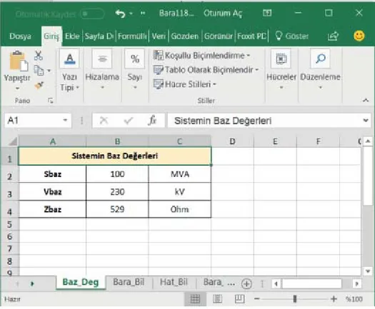
This study focused on designing a new program that facilitates data input in the load flow program. Data input was performed using Excel, and transferred to Matlab R2015b. The load flow solution was obtained by forming the coding of the program as distinct subprograms and results were printed to a file. The data input sheets in Excel are given in Figures 1, 2 and 3. Power base (Sbase), voltage base (Vbase) and impedance base (Zbase) values used in the system solution are entered in the Baz_Deg sheet in Figure 1.
International Journal of Research and Development, Vol.9, No.3, December 2017, Special Issue
Figure 1. System base values input sheet
The bus numbers, generator bus types (UreTip), bus types (BusTip), active power generation limits of generators (Pmin, Pmax), initial value of active power generation (PGen), reactive power generation limits of generators (Qmin, Qmax), initial value of reactive power generation (QGen), active and reactive load values at buses (Pload, Qload), voltage limits of buses (Vmin, Vmax), voltage values of voltage-controlled buses (Vbus) and bus angles (Açı) used in the solution of the problem are entered in the Bus_Bil sheet given in Figure 2.
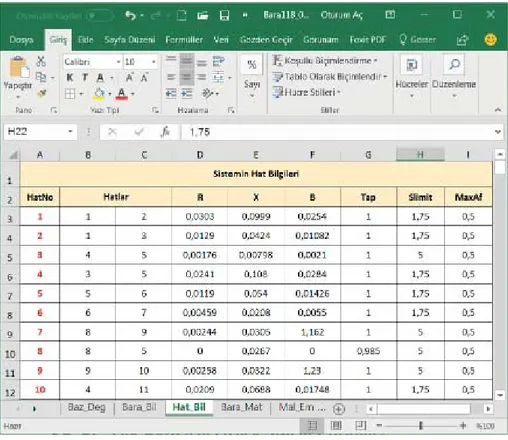
The line numbers, serial impedance between lines (R), parallel admittance (X), capacitance values (B), transformer transfer ratio (Tap), transmission line carrying capacities (Slimit) and maximum angle difference between buses (MaxAf), which are the transmission line information of the system, are entered in the Hat_Bil sheet given in Figure 3.
Figure 3. System line information input sheet
In this design used to input system data, the program can easily be integrated into the new state by adding a sheet or column to the data file for additional information required for a new problem or a new system.
After the system data is uploaded to an Excel file, the following code block generated in Matlab is used to convert the data into a matrix form with a .mat extension. The data converted into a matrix form is uploaded to the Matlab application and their load flow is performed and results are printed.
4. SAMPLE SYSTEM SOLUTION
format compact clear, clc s = 'Bara118_0'; file = [s,'.mat']; if exist(file,'file') ~= 2 tic f = [s,'.xlsx']; Baz = xlsread(f,1); Bara = xlsread(f,2); Hat = xlsread(f,3); BMat = xlsread(f,4); MalEmKat = xlsread(f,5); clear sf save(file) toc end Data = load(file)
International Journal of Research and Development, Vol.9, No.3, December 2017, Special Issue
A sample power system consisting of IEEE 118 buses, 54 thermal power generation units and 179 transmission lines referred to as single-line diagram in Appendix Figure 1 was selected in order to test the load flow analysis in this section (Power Systems Test Case Archieve, 2017), (MatPower, 2017), (Zahlay, 2016).
This system is one of the high dimensional systems in the literature. Bus no 69 in the system is a slack bus and its voltage is
0
1.035 0 pu. All 54 generators in the system consist of voltage-controlled buses. 9 transmission lines in the system have
transformers. The base values of the system were designated as Sbase=100 MVA, Ubase=230 kVA and Zbase=529 Ohm.
Appendix Table 1 shows the serial impedance, parallel admittance, capacitance values, transformer transfer ratios and line carrying capacities of the nominal π equivalent circuits of the transmission lines in the sample system. 91 buses and their active and reactive load values that remain unchanged at a period of time in the system are given as pu in Appendix Table 2. Appendix Table 3 presents the initial values of the load flow of the generation units. The 54 generators in the system are voltage-controlled buses and the bus voltages of these buses are kept constant at the values given in Appendix Table 3. The working limit values of the generation units in the system are given in Appendix Table 4 (Power Systems Test Case Archieve, 2017), (MatPower,2017), (Zahlay, 2016)
The bus voltage magnitude and angle values (Vk, δk), active and reactive power generation values (Pk, Qk) as pu in the generation
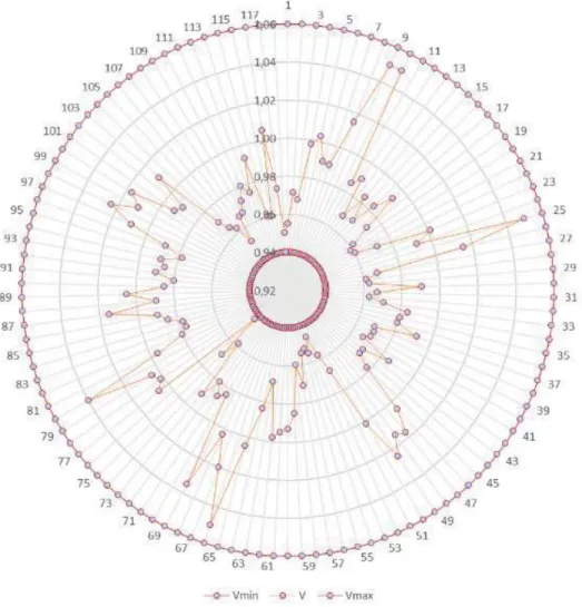
units and transmission line losses obtained from AC load flow in the sample system are given in Annex Table 5. The transmission line losses that occured as a result of AC load flow in the sample system were Ploss=0,614601 pu. The voltage magnitudes of the buses in the system ranged from 0.94 to 1.06 pu. The voltage profile of all the buses showing this state is given in Figure 4. The load flow solution time of the large size sample system at the work statiton with Intel Xeon E5-2637 v4 3.50 GHz processor and 128 GB RAM memory was 0.0719492 sec.
Figure 4. Voltage profile of IEEE 118 bus system at solution point 5. CONCLUSION
In this study, the Newton-Raphson method was used to perform load flow analysis and the new program facilitates the data input for the process. On a different sample system, this new data input method can be used to provide data input without running the
load flow program. This new method makes it easier to correctly input data for the solutions to high-dimensional systems. It also prevents erroneous data input. The data input innovation developed in this study can also be improved for future studies and used for economic power distribution and short term hydrothermal coordination problems.
ACKNOWLEDGMENT
This work was supported by the Dumlupınar University Scientific Research Projects Commission under the 2016-65 project.
REFERENCES
Allan, R.N. and Al-Shakarchi, M.R.G. “Probabilistic techniques in a.c. load-flow analysis”, Proceedings of the Institution of Electrical Engineers, vol. 124, no. 2, pp. 154-160, February 1977.
Dagur, D., Parimi, M. and Wagh, S.R., “Prediction of cascade failure using probabilistic approach with AC load flow” IEEE Innovative Smart Grid Technologies-Asia, 2014, pp. 542-547.
Kothari, D.P. and Dhillon, J.S., Power System Optimization, PHI, New Delhi, 2007.
Özyön S., The application of genetic algorithm to some environmental economic power dispatch problems, Msc. Thesis, Dumlupınar University, Kütahya, 2009.
Panosyan, A. and Oswald, B.R., “Modified Newton-Raphson load flow analysis for integrated AC/DC power systems” 39th International Universities Power Engineering Conference, 2004, pp. 1223-1227.
Power Systems Test Case Archive. (n.d.). Retrieved September 12, 2017, from https://www2.ee.washington.edu/research/pstca/ MatPower, Retrieved September 12, 2017, from http://www.pserc.cornell.edu/matpower/
Revanthi, A.A., Load flow and optimal power flow analysis using evolutionary computational techniques, Phd Thesis, Anna University, Faculty of Electrical and Electronics Engineering, 2008.
Rossoni, P., Rosa, W.M. and Belati, E.A. “Linearized AC load flow applied to analysis in electric power systems”, IEEE Latin America Transactions, vol. 14, no. 9, pp. 4048-4053, September 2016.
Wood, A.J., Wollenberg, B.F. and Sheble, G.B., Power Generation Operation and Control, IEEE & Wiley, Third Edition, USA, 2013.
Zahlay, F.D., Strategies, Methods and Tools for Solving Long-term Transmission Expansion Planning in Large-scale Power Systems, Ph.D. Thesis, Spain, 2016.
213 Appendix 1 2 3 4 5 6 7 8 9 10 27 114 28 29 12 11 16 13 32 115 26 113 14 15 17 30 19 18 20 21 22 23 25 117 33 40 39 41 42 53 54 52 34 36 43 44 45 46 47 38 48 37 49 50 51 58 57 56 55 59 63 60 64 61 62 67 65 66 68 69 V69 = 1.035 0o 116 79 78 70 24 72 73 71 74 75 77 76 118 82 83 84 85 88 89 86 87 90 92 111 110 112 109 108 103 104 105 107 100 91 101 102 93 94 95 96 97 98 99 80 81 106 Thermal Generation Unit Load GT GT GT GT GT GT GT GT GT GT 31 GT GT GT GT GT GT GT GT GT GT G T GT GT GT GT GT GT GT GT GT GT GT GT GT GT GT GT GT GT GT GT GT GT GT GT GT GT GT GT GT GT GT GT GT 35 GT
IEEE Test System - 118 bus - 179 transmission line - 54 Thermal generation unit - 91 load bus
Appendix Table 1. Values of nominal π equivalent circuits of transmission lines in the sample system
Line no
From
bus To bus R (pu) X (pu) B (pu) Tap SL
max 1 1 2 0,03030 0,09990 0,02540 - 1,750 2 1 3 0,01290 0,04240 0,01082 - 1,750 3 4 5 0,00176 0,00798 0,00210 - 5,000 4 3 5 0,02410 0,10800 0,02840 - 1,750 5 5 6 0,01190 0,05400 0,01426 - 1,750 6 6 7 0,00459 0,02080 0,00550 - 1,750 7 8 9 0,00244 0,03050 1,16200 - 5,000 8 8 5 - 0,02670 - 0,985 5,000 9 9 10 0,00258 0,03220 1,23000 - 5,000 10 4 11 0,02090 0,06880 0,01748 - 1,750 11 5 11 0,02030 0,06820 0,01738 - 1,750 12 11 12 0,00595 0,01960 0,00502 - 1,750 13 2 12 0,01870 0,06160 0,01572 - 1,750 14 3 12 0,04840 0,16000 0,04060 - 1,750 15 7 12 0,00862 0,03400 0,00874 - 1,750 16 11 13 0,02225 0,07310 0,01876 - 1,750 17 12 14 0,02150 0,07070 0,01816 - 1,750 18 13 15 0,07440 0,24440 0,06268 - 1,750 19 14 15 0,05950 0,19500 0,05020 - 1,750 20 12 16 0,02120 0,08340 0,02140 - 1,750 21 15 17 0,01320 0,04370 0,04440 - 5,000 22 16 17 0,04540 0,18010 0,04660 - 1,750 23 17 18 0,01230 0,05050 0,01298 - 1,750 24 18 19 0,01119 0,04930 0,01142 - 1,750 25 19 20 0,02520 0,11700 0,02980 - 1,750 26 15 19 0,01200 0,03940 0,01010 - 1,750 27 20 21 0,01830 0,08490 0,02160 - 1,750 28 21 22 0,02090 0,09700 0,02460 - 1,750 29 22 23 0,03420 0,15900 0,04040 - 1,750 30 23 24 0,01350 0,04920 0,04980 - 1,750 31 23 25 0,01560 0,08000 0,08640 - 5,000 32 26 25 - 0,03820 - 0,960 5,000 33 25 27 0,03180 0,16300 0,17640 - 5,000 34 27 28 0,01913 0,08550 0,02160 - 1,750 35 28 29 0,02370 0,09430 0,02380 - 1,750 36 30 17 - 0,03880 - 0,960 5,000 37 8 30 0,00431 0,05040 0,51400 - 1,750 38 26 30 0,00799 0,08600 0,90800 - 5,000 39 17 31 0,04740 0,15630 0,03990 - 1,750 40 29 31 0,01080 0,03310 0,00830 - 1,750 41 23 32 0,03170 0,11530 0,11730 - 1,40 42 31 32 0,02980 0,09850 0,02510 - 1,750 43 27 32 0,02290 0,07550 0,01926 - 1,750 44 15 33 0,03800 0,12440 0,03194 - 1,750 45 19 34 0,07520 0,24700 0,06320 - 1,750 46 35 36 0,00224 0,01020 0,00268 - 1,750 47 35 37 0,01100 0,04970 0,01318 - 1,750 48 33 37 0,04150 0,14200 0,03660 - 1,750 49 34 36 0,00871 0,02680 0,00568 - 1,750 50 34 37 0,00256 0,00940 0,00984 - 5,000 51 38 37 - 0,03750 - 0,935 5,000
International Journal of Research and Development, Vol.9, No.3, December 2017, Special Issue 215 53 37 40 0,05930 0,16800 0,04200 - 1,750 54 30 38 0,00464 0,05400 0,42200 - 1,750 55 39 40 0,01840 0,06050 0,01552 - 1,750 56 40 41 0,01450 0,04870 0,01222 - 1,750 57 40 42 0,05550 0,18300 0,04660 - 1,750 58 41 42 0,04100 0,13500 0,03440 - 1,750 59 43 44 0,06080 0,24540 0,06068 - 1,750 60 34 43 0,04130 0,16810 0,04226 - 1,750 61 44 45 0,02240 0,09010 0,02240 - 1,750 62 45 46 0,04000 0,13560 0,03320 - 1,750 63 46 47 0,03800 0,12700 0,03160 - 1,750 64 46 48 0,06010 0,18900 0,04720 - 1,750 65 47 49 0,01910 0,06250 0,01604 - 1,750 66 42 49 0,03575 0,16150 0,17200 - 2,300 67 45 49 0,06840 0,18600 0,04440 - 1,750 68 48 49 0,01790 0,05050 0,01258 - 1,750 69 49 50 0,02670 0,07520 0,01874 - 1,750 70 49 51 0,04860 0,13700 0,03420 - 1,750 71 51 52 0,02030 0,05880 0,01396 - 1,750 72 52 53 0,04050 0,16350 0,04058 - 1,750 73 53 54 0,02630 0,12200 0,03100 - 1,750 74 49 54 0,03993 0,14507 0,14680 - 2,300 75 54 55 0,01690 0,07070 0,02020 - 1,750 76 54 56 0,00275 0,00955 0,00732 - 1,750 77 55 56 0,00488 0,01510 0,00374 - 1,750 78 56 57 0,03430 0,09660 0,02420 - 1,750 79 50 57 0,04740 0,13400 0,03320 - 1,750 80 56 58 0,03430 0,09660 0,02420 - 1,750 81 51 58 0,02550 0,07190 0,01788 - 1,750 82 54 59 0,05030 0,22930 0,05980 - 1,750 83 56 59 0,04070 0,12243 0,11050 - 2,300 84 55 59 0,04739 0,21580 0,05646 - 1,750 85 59 60 0,03170 0,14500 0,03760 - 1,750 86 59 61 0,03280 0,15000 0,03880 - 1,750 87 60 61 0,00264 0,01350 0,01456 - 5,000 88 60 62 0,01230 0,05610 0,01468 - 1,750 89 61 62 0,00824 0,03760 0,00980 - 1,750 90 63 59 - 0,03860 - 0,960 5,000 91 63 64 0,00172 0,02000 0,21600 - 5,000 92 64 61 - 0,02680 - 0,985 5,000 93 38 65 0,00901 0,09860 1,04600 - 5,000 94 64 65 0,00269 0,03020 0,38000 - 5,000 95 49 66 0,00900 0,04595 0,04960 - 8,000 96 62 66 0,04820 0,21800 0,05780 - 1,750 97 62 67 0,02580 0,11700 0,03100 - 1,750 98 65 66 - 0,03700 - 0,935 5,000 99 66 67 0,02240 0,10150 0,02682 - 1,750 100 65 68 0,00138 0,01600 0,63800 - 5,000 101 47 69 0,08440 0,27780 0,07092 - 1,750 102 49 69 0,09850 0,32400 0,08280 - 1,750 103 68 69 - 0,03700 - 0,935 5,000 104 69 70 0,03000 0,12700 0,12200 - 5,000 105 24 70 0,00221 0,41150 0,10198 - 1,750 106 70 71 0,00882 0,03550 0,00878 - 1,750 107 24 72 0,04880 0,19600 0,04880 - 1,750
108 71 72 0,04460 0,18000 0,04444 - 1,750 109 71 73 0,00866 0,04540 0,01178 - 1,750 110 70 74 0,04010 0,13230 0,03368 - 1,750 111 70 75 0,04280 0,14100 0,03600 - 1,750 112 69 75 0,04050 0,12200 0,12400 - 5,000 113 74 75 0,01230 0,04060 0,01034 - 1,750 114 76 77 0,04440 0,14800 0,03680 - 1,750 115 69 77 0,03090 0,10100 0,10380 - 1,750 116 75 77 0,06010 0,19990 0,04978 - 1,750 117 77 78 0,00376 0,01240 0,01264 - 1,750 118 78 79 0,00546 0,02440 0,00648 - 1,750 119 77 80 0,01088 0,03321 0,07000 - 8,000 120 79 80 0,01560 0,07040 0,01870 - 1,750 121 68 81 0,00175 0,02020 0,80800 - 5,000 122 81 80 - 0,03700 - 0,935 5,000 123 77 82 0,02980 0,08530 0,08174 - 2,000 124 82 83 0,01120 0,03665 0,03796 - 2,000 125 83 84 0,06250 0,13200 0,02580 - 1,750 126 83 85 0,04300 0,14800 0,03480 - 1,750 127 84 85 0,03020 0,06410 0,01234 - 1,750 128 85 86 0,03500 0,12300 0,02760 - 5,000 129 86 87 0,02828 0,20740 0,04450 - 5,000 130 85 88 0,02000 0,10200 0,02760 - 1,750 131 85 89 0,02390 0,17300 0,04700 - 1,750 132 88 89 0,01390 0,07120 0,01934 - 5,000 133 89 90 0,01638 0,06517 0,15880 - 8,000 134 90 91 0,02540 0,08360 0,02140 - 1,750 135 89 92 0,00799 0,03829 0,09620 - 8,000 136 91 92 0,03870 0,12720 0,03268 - 1,750 137 92 93 0,02580 0,08480 0,02180 - 1,750 138 92 94 0,04810 0,15800 0,04060 - 1,750 139 93 94 0,02230 0,07320 0,01876 - 1,750 140 94 95 0,01320 0,04340 0,01110 - 1,750 141 80 96 0,03560 0,18200 0,04940 - 1,750 142 82 96 0,01620 0,05300 0,05440 - 1,750 143 94 96 0,02690 0,08690 0,02300 - 1,750 144 80 97 0,01830 0,09340 0,02540 - 1,750 145 80 98 0,02380 0,10800 0,02860 - 1,750 146 80 99 0,04540 0,20600 0,05460 - 2,000 147 92 100 0,06480 0,29500 0,04720 - 1,750 148 94 100 0,01780 0,05800 0,06040 - 1,750 149 95 96 0,01710 0,05470 0,01474 - 1,750 150 96 97 0,01730 0,08850 0,02400 - 1,750 151 98 100 0,03970 0,17900 0,04760 - 1,750 152 99 100 0,01800 0,08130 0,02160 - 1,750 153 100 101 0,02770 0,12620 0,03280 - 1,750 154 92 102 0,01230 0,05590 0,01464 - 1,750 155 101 102 0,02460 0,11200 0,02940 - 1,750 156 100 103 0,01600 0,05250 0,05360 - 5,000 157 100 104 0,04510 0,20400 0,05410 - 1,750 158 103 104 0,04660 0,15840 0,04070 - 1,750 159 103 105 0,05350 0,16250 0,04080 - 1,750 160 100 106 0,06050 0,22900 0,06200 - 1,750 161 104 105 0,00994 0,03780 0,00986 - 1,750
International Journal of Research and Development, Vol.9, No.3, December 2017, Special Issue 217 163 105 107 0,05300 0,18300 0,04720 - 1,750 164 105 108 0,02610 0,07030 0,01844 - 1,750 165 106 107 0,05300 0,18300 0,04720 - 1,750 166 108 109 0,01050 0,02880 0,00760 - 1,750 167 103 110 0,03906 0,18130 0,04610 - 1,750 168 109 110 0,02780 0,07620 0,02020 - 1,750 169 110 111 0,02200 0,07550 0,02000 - 1,750 170 110 112 0,02470 0,06400 0,06200 - 1,750 171 17 113 0,00913 0,03010 0,00768 - 1,750 172 32 113 0,06150 0,20300 0,05180 - 5,000 173 32 114 0,01350 0,06120 0,01628 - 1,750 174 27 115 0,01640 0,07410 0,01972 - 1,750 175 114 115 0,00230 0,01040 0,00276 - 1,750 176 68 116 0,00034 0,00405 0,16400 - 5,000 177 12 117 0,03290 0,14000 0,03580 - 1,750 178 75 118 0,01450 0,04810 0,01198 - 1,750 179 76 118 0,01640 0,05440 0,01356 - 1,750
Appendix Table 2. Active and reactive load values in the sample system.
Bus
No Pload (pu) Qload (pu)
Bus
No Pload (pu) Qload (pu)
1 0,5100 0,2700 60 0,7800 0,0300 2 0,2000 0,0900 61 - - 3 0,3900 0,1000 62 0,7700 0,1400 4 0,3900 0,1200 63 - - 5 - - 64 - - 6 0,5200 0,2200 65 - - 7 0,1900 0,0200 66 0,3900 0,1800 8 0,2800 0,0000 67 0,2800 0,0700 9 - - 68 - - 10 - - 69 - - 11 0,7000 0,2300 70 0,6600 0,2000 12 0,4700 0,1000 71 - - 13 0,3400 0,1600 72 0,1200 - 14 0,1400 0,0100 73 0,0600 - 15 0,9000 0,3000 74 0,6800 0,2700 16 0,2500 0,1000 75 0,4700 0,1100 17 0,1100 0,0300 76 0,6800 0,3600 18 0,6000 0,3400 77 0,6100 0,2800 19 0,4500 0,2500 78 0,7100 0,2600 20 0,1800 0,0300 79 0,3900 0,3200 21 0,1400 0,0800 80 1,3000 0,2600 22 0,1000 0,0500 81 - - 23 0,0700 0,0300 82 0,5400 0,2700 24 0,1300 - 83 0,2000 0,1000 25 - - 84 0,1100 0,0700 26 - - 85 0,2400 0,1500 27 0,7100 0,1300 86 0,2100 0,1000 28 0,1700 0,0700 87 - - 29 0,2400 0,0400 88 0,4800 0,1000 30 - - 89 - - 31 0,4300 0,2700 90 1,6300 0,4200 32 0,5900 0,2300 91 0,1000 - 33 0,2300 0,0900 92 0,6500 0,1000 34 0,5900 0,2600 93 0,1200 0,0700
35 0,3300 0,0900 94 0,3000 0,1600 36 0,3100 0,1700 95 0,4200 0,3100 37 - - 96 0,3800 0,1500 38 - - 97 0,1500 0,0900 39 0,2700 0,1100 98 0,3400 0,0800 40 0,6600 0,2300 99 0,4200 - 41 0,3700 0,1000 100 0,3700 0,1800 42 0,9600 0,2300 101 0,2200 0,1500 43 0,1800 0,0700 102 0,0500 0,0300 44 0,1600 0,0800 103 0,2300 0,1600 45 0,5300 0,2200 104 0,3800 0,2500 46 0,2800 0,1000 105 0,3100 0,2600 47 0,3400 - 106 0,4300 0,1600 48 0,2000 0,1100 107 0,5000 0,1200 49 0,8700 0,3000 108 0,0200 0,0100 50 0,1700 0,0400 109 0,0800 0,0300 51 0,1700 0,0800 110 0,3900 0,3000 52 0,1800 0,0500 111 - - 53 0,2300 0,1100 112 0,6800 0,1300 54 1,1300 0,3200 113 0,0600 - 55 0,6300 0,2200 114 0,0800 0,0300 56 0,8400 0,1800 115 0,2200 0,0700 57 0,1200 0,0300 116 1,8400 - 58 0,1200 0,0300 117 0,2000 0,0800 59 2,7700 1,1300 118 0,3300 0,1500
Total Load Pload: 42,4200 Qload: 14,3800
Appendix Table 3. AC load flow initial values of the generation units in the sample system
Gen. Unit Bus Pi (pu) Qi (pu) V (pu) Gen. Unit Bus Pi (pu) Qi (pu) V (pu) 1 1 0,500 0,075 0,995 28 65 2,000 1,000 1,005 2 4 0,500 1,500 0,998 29 66 2,000 1,000 1,050 3 6 0,500 0,250 0,990 30 69 - - 1,035 4 8 0,500 1,500 1,015 31 70 0,500 0,150 0,984 5 10 2,000 1,000 1,050 32 72 0,500 0,500 0,980 6 12 1,000 0,600 0,990 33 73 0,500 0,500 0,991 7 15 0,500 0,150 0,970 34 74 0,500 0,045 0,958 8 18 0,500 0,250 0,973 35 76 0,500 0,120 0,943 9 19 0,500 0,120 0,962 36 77 0,500 0,350 1,006 10 24 0,500 1,500 0,992 37 80 2,000 1,400 1,040 11 25 1,000 0,700 1,050 38 85 0,500 0,120 0,985 12 26 2,000 5,000 1,015 39 87 0,500 5,000 1,015 13 27 0,500 1,500 0,968 40 89 2,000 1,500 1,005 14 31 0,500 1,500 0,967 41 90 0,500 1500 0,985 15 32 0,500 0,210 0,963 42 91 0,500 0,500 0,980 16 34 0,500 0,120 0,984 43 92 0,500 0,045 0,990 17 36 0,500 0,120 0,980 44 99 0,500 0,500 1,010 18 40 0,500 1,500 0,970 45 100 1,000 0,750 1,017 19 42 0,500 1,500 0,985 46 103 0,500 0,200 1,010 20 46 0,500 0,500 1,005 47 104 0,500 0,120 0,971 21 49 1,000 1,000 1,025 48 105 0,500 0,120 0,965 22 54 0,500 1,500 0,955 49 107 0,500 1,000 0,952 23 55 0,500 0,120 0,952 50 110 0,500 0,120 0,973 24 56 0,500 0,075 0,954 51 111 0,500 5,000 0,980
International Journal of Research and Development, Vol.9, No.3, December 2017, Special Issue
219
26 61 1,000 1,500 0,995 53 113 0,500 1,000 0,993
27 62 0,500 0,100 0,998 54 116 0,500 5,000 1,005
Appendix Table 4. Operating limit values of generation units in the sample system.
Gen. Unit Bus Pmin (pu) Pmax (pu) Qmin (pu) Qmax (pu) Vmin (pu) Vmax (pu) 1 1 0,0000 1,0000 -0,0500 0,1500 0,9400 1,0600 2 4 0,0000 1,0000 -3,0000 3,0000 0,9400 1,0600 3 6 0,0000 1,0000 -0,1300 0,5000 0,9400 1,0600 4 8 0,0000 1,0000 -3,0000 3,0000 0,9400 1,0600 5 10 0,0000 5,5000 -1,4700 2,0000 0,9400 1,0600 6 12 0,0000 1,8500 -0,3500 1,2000 0,9400 1,0600 7 15 0,0000 1,0000 -0,1000 0,3000 0,9400 1,0600 8 18 0,0000 1,0000 -0,1600 0,5000 0,9400 1,0600 9 19 0,0000 1,0000 -0,0800 0,2400 0,9400 1,0600 10 24 0,0000 1,0000 -3,0000 3,0000 0,9400 1,0600 11 25 0,0000 3,2000 -0,4700 1,4000 0,9400 1,0600 12 26 0,0000 4,1400 10,0000 - 10,0000 0,9400 1,0600 13 27 0,0000 1,0000 -3,0000 3,0000 0,9400 1,0600 14 31 0,0000 1,0700 -3,0000 3,0000 0,9400 1,0600 15 32 0,0000 1,0000 -0,1400 0,4200 0,9400 1,0600 16 34 0,0000 1,0000 -0,0800 0,2400 0,9400 1,0600 17 36 0,0000 1,0000 -0,0800 0,2400 0,9400 1,0600 18 40 0,0000 1,0000 -3,0000 3,0000 0,9400 1,0600 19 42 0,0000 1,0000 -3,0000 3,0000 0,9400 1,0600 20 46 0,0000 1,1900 -1,0000 1,0000 0,9400 1,0600 21 49 0,0000 3,0400 -0,8500 2,1000 0,9400 1,0600 22 54 0,0000 1,4800 -3,0000 3,0000 0,9400 1,0600 23 55 0,0000 1,0000 -0,0800 0,2300 0,9400 1,0600 24 56 0,0000 1,0000 -0,0800 0,1500 0,9400 1,0600 25 59 0,0000 2,5500 -0,6000 1,8000 0,9400 1,0600 26 61 0,0000 2,6000 -1,0000 3,0000 0,9400 1,0600 27 62 0,0000 1,0000 -0,2000 0,2000 0,9400 1,0600 28 65 0,0000 4,9100 -0,6700 2,0000 0,9400 1,0600 29 66 0,0000 4,9200 -0,6700 2,0000 0,9400 1,0600 30 69 0,0000 8,0520 -3,0000 3,0000 0,9400 1,0600 31 70 0,0000 1,0000 -0,1000 0,3200 0,9400 1,0600 32 72 0,0000 1,0000 -1,0000 1,0000 0,9400 1,0600 33 73 0,0000 1,0000 -1,0000 1,0000 0,9400 1,0600 34 74 0,0000 1,0000 -0,0600 0,0900 0,9400 1,0600 35 76 0,0000 1,0000 -0,0800 0,2300 0,9400 1,0600 36 77 0,0000 1,0000 -0,2000 0,7000 0,9400 1,0600 37 80 0,0000 5,7700 -1,6500 2,8000 0,9400 1,0600 38 85 0,0000 1,0000 -0,0800 0,2300 0,9400 1,0600 39 87 0,0000 1,0400 -1,0000 10,0000 0,9400 1,0600 40 89 0,0000 7,0700 -2,1000 3,0000 0,9400 1,0600 41 90 0,0000 1,0000 -3,0000 3,0000 0,9400 1,0600 42 91 0,0000 1,0000 -1,0000 1,0000 0,9400 1,0600 43 92 0,0000 1,0000 -0,0300 0,0900 0,9400 1,0600 44 99 0,0000 1,0000 -1,0000 1,0000 0,9400 1,0600 45 100 0,0000 3,5200 -0,5000 1,5500 0,9400 1,0600 46 103 0,0000 1,4000 -0,1500 0,4000 0,9400 1,0600
47 104 0,0000 1,0000 -0,0800 0,2300 0,9400 1,0600 48 105 0,0000 1,0000 -0,0800 0,2300 0,9400 1,0600 49 107 0,0000 1,0000 -2,0000 2,0000 0,9400 1,0600 50 110 0,0000 1,0000 -0,0800 0,2300 0,9400 1,0600 51 111 0,0000 1,3600 -1,0000 10,0000 0,9400 1,0600 52 112 0,0000 1,0000 -1,0000 10,0000 0,9400 1,0600 53 113 0,0000 1,0000 -1,0000 2,0000 0,9400 1,0600 54 116 0,0000 1,0000 10,0000 - 10,0000 0,9400 1,0600
Appendix Table 5. The values obtained as a result of AC load flow of all the buses in the sample system.
Bus
No V (pu) G (R)
Pgen
(pu) Q
gen
(pu) Bus No V (pu) G (R) Pgen (pu) Q gen (pu) 1 0,9550 0,0326 - 0,5000 0,1882 - 60 0,9932 0,1631 - - - 2 0,9715 0,0401 - - - 61 0,9950 0,1496 - 1,0000 0,3185 -3 0,9678 0,0351 - - - 62 0,9980 0,1523 - 0,5000 0,1092 -4 0,9980 0,0012 - 0,5000 0,3627 - 63 0,9688 0,1656 - - - 5 1,0028 0,0007 - - 64 0,9836 0,1365 - - - 6 0,9900 0,0185 - 0,5000 0,0169 65 1,0050 0,0788 - 2,0000 0,8208 7 0,9893 0,0265 - - - 66 1,0500 0,1034 - 2,0000 0,1283 8 1,0150 0,0428 0,5000 0,2691 - 67 1,0200 0,1396 - - - 9 1,0500 0,0973 - - 68 1,0032 0,0699 - - - 10 1,0500 0,1560 2,0000 0,7807 - 69 1,0350 0,0000 4,5346 0,5042 -11 0,9855 0,0324 - - - 70 0,9840 0,0156 0,5000 0,1494 -12 0,9900 0,0331 - 1,0000 0,8467 71 0,9869 0,0444 - - 13 0,9687 0,0519 - - - 72 0,9800 0,1112 0,5000 0,2242 -14 0,9836 0,0426 - - - 73 0,9910 0,0647 0,5000 0,0042 15 0,9700 0,0394 - 0,5000 0,0458 - 74 0,9580 0,0318 - 0,5000 0,1250 -16 0,9833 0,0397 - - - 75 0,9686 0,0436 - - - 17 0,9933 0,0111 - - - 76 0,9430 0,0703 - 0,5000 0,1319 -18 0,9730 0,0244 - 0,5000 0,1853 77 1,0060 0,0802 - 0,5000 0,1428 19 0,9620 0,0345 - 0,5000 0,2941 - 78 1,0015 0,0898 - - - 20 0,9588 0,0335 - - - 79 1,0043 0,0931 - - - 21 0,9606 - - - 80 1,0400 - 2,0000 1,7349
International Journal of Research and Development, Vol.9, No.3, December 2017, Special Issue 221 22 0,9723 0,0164 - - 81 0,9962 0,0736 - - - 23 1,0012 0,0834 - - 82 0,9801 0,0946 - - - 24 0,9920 0,0978 0,5000 0,2436 - 83 0,9767 0,0823 - - - 25 1,0500 0,1334 1,0000 0,5919 84 0,9775 0,0538 - - - 26 1,0150 0,1484 2,0000 0,0189 - 85 0,9850 0,0344 - 0,5000 0,0683 -27 0,9680 0,0374 0,5000 0,1697 - 86 0,9898 0,0027 - - 28 0,9616 0,0154 - - 87 1,0150 0,1038 0,5000 0,0570 29 0,9631 0,0072 - - 88 0,9893 0,0430 - - - 30 0,9907 0,0161 - - 89 1,0050 0,0157 - 2,0000 0,4733 31 0,9670 0,0124 0,5000 0,2063 90 0,9850 0,0655 - 0,5000 0,4176 32 0,9630 0,0351 0,5000 0,3544 - 91 0,9800 0,0304 - 0,5000 0,2758 -33 0,9709 0,0858 - - - 92 0,9900 0,0398 - 0,5000 0,3647 -34 0,9840 0,1063 - 0,5000 0,2759 - 93 0,9858 0,0624 - - - 35 0,9807 0,1089 - - - 94 0,9889 0,0741 - - - 36 0,9800 0,1062 - 0,5000 0,0869 - 95 0,9781 0,0917 - - - 37 0,9921 0,1060 - - - 96 0,9885 0,0953 - - - 38 0,9694 0,0608 - - - 97 1,0093 0,0940 - - - 39 0,9705 0,1643 - - - 98 1,0234 0,0879 - - - 40 0,9700 0,1828 - 0,5000 0,1216 99 1,0100 0,0464 - 0,5000 0,2875 -41 0,9668 0,2044 - 0,0000 0,0000 100 1,0170 0,0433 - 1,0000 1,2848 42 0,9850 0,2143 - 0,5000 0,1998 101 0,9927 0,0570 - - - 43 0,9704 0,1649 - - - 102 0,9901 0,0474 - - - 44 0,9704 0,2063 - - - 103 1,0100 0,0200 - 0,5000 0,5789 45 0,9782 0,2071 - - - 104 0,9710 0,0125 - 0,5000 0,1276 -46 1,0050 0,1707 - 0,5000 0,0329 105 0,9650 0,0128 - 0,5000 0,1532 -47 1,0173 0,1611 - - - 106 0,9624 0,0345 - - - 48 1,0149 0,1778 - - - 107 0,9520 0,0201 - 0,5000 0,0441 -49 1,0250 0,1714 - 1,0000 1,3987 108 0,9664 0,0016 - - - 50 1,0015 0,2010 - - - 109 0,9672 0,0036 - -
51 0,9677 0,2393 - - - 110 0,9730 0,0233 0,5000 0,0481 -52 0,9577 0,2542 - - - 111 0,9800 0,0639 0,5000 0,0540 -53 0,9464 0,2665 - - - 112 0,9750 0,0085 0,5000 0,2021 54 0,9550 0,2471 - 0,5000 0,0191 113 0,9930 0,0064 0,5000 0,0190 -55 0,9520 0,2456 - 0,5000 0,0980 - 114 0,9601 0,0263 - - 56 0,9540 0,2461 - 0,5000 0,2127 - 115 0,9600 0,0256 - - 57 0,9710 0,2337 - - - 116 1,0050 0,0755 - 0,5000 0,4698 58 0,9595 0,2474 - - - 117 0,9738 0,0600 - - - 59 0,9850 0,2213 - 1,0000 0,8911 118 0,9501 0,0640 - - - Total Active
Power 43,034601 Total P Load 42,420000 Ploss 0,614601
Total Reactive Power 4,419482 Total Q Load 14,380000 Qloss -9,961833 Time (sec): 0,034583