Selçuk J. Appl. Math. Selçuk Journal of Vol. 11. No.2. pp. 63-70, 2010 Applied Mathematics
Average Edge-Distance in Graphs Mehmet Ali Balcı, Pınar Dündar
Ege University Faculty of Science Department of Mathematics, 35100 Bornova-˙Izmir Türkiye
e-mail: m ehm et.ali.balci@ ege.edu.tr
Ege University Faculty of Science Department of Mathematics, 35100 Bornova-˙Izmir Türkiye
e-mail: pinar.dundar@ ege.edu.tr
Received Date: November 24, 2009 Accepted Date: December 14, 2010
Abstract. The average edge-distance of a connected graph G is the average of the distance between all pairs of edges of G. In this work we give the average edge-distance of a graph, a new vulnerability measure. We also find sub and upper bounds for average edge-distance and give a polynomial time algorithm which calculates the average edge-distance of a graph.
Key words: Graph theory, edge-distance and average edge-distance. 2000 Mathematics Subject Classification. 05C12, 05C76.
1. Introduction
Vulnerability is the most important concept in any communication network. The resistance of a network after any disruption is considered as vulnerability value. In a network, this disruption does not only can take place on its centers also sometimes on its links. In this case the vulnerability measures given on links (edges) play an important role in the construction of communication networks. A communication network can be modeled by a graph whose vertices represent the stations and whose edges represent the lines of communication. A graph G is denoted by G = (V (G), E (G)), where V (G) and E (G) are vertices and edges sets of G, respectively. All graphs in this paper are simple, finite, undirected and without multiple edges. In graph theory, many graph parameters have been used widely in the past to describe the stability of a graph. For example connectivity is one of the first and the most important measures of vulnerability. Latterly it has been observed that these measures were not enough to compare two network models having the same values of some of these parameters.
For example the vertex connectivity of a path graph and a star graph which have the same order are equal. Also their edge connectivities are equal. In this case we need extra measurements to decide which model is suitable than the others. The definition of average distance is given by P. Dankelmann in 1997. [3,4]. In this work we define average edge-distance 0 a graph which is a new
vulnerability measure given on edges of a graph.
Definition 1.1. Let the nodes of , be labeled as 1 2 3 . The
adja-cency matrix = () = [] of is the binary matrix of order [7].
=
½
1 if is adjacent with
0 otherwise
Definition 1.2. For a connected graph , the distance d (u, v) between two vertices u and v is defined as the minimum lengths of the − paths [2]. Definition 1.3. Let be a connected graph whose nodes are labeled 12.
The distance matrix () = [] of G has = ( ) is the distance between
and . Thus () is a symmetric × matrix [2].
Definition 1.4. Let be a connected graph of order . The average dis-tance () of is defined as () = µ 2 ¶−1 P {}⊂ ( ) where ( )
denotes the distance between the vertices and [3,4].
Definition 1.5. The degree of a vertex is the number of edges at and is denoted by () [5].
Definition 1.6. The number () = min {() | ∈ () } is the minimum degree of [5].
Definition 1.7. The number () = 1 | |
P
∈
() is the average degree of [5].
Definition 1.8. Let 1 and 2 be two edges of the graph . If they have one
common vertex they are called neighbour edges of [1].
Definition 1.9. The degree of an edge = ( ) is the number of edge which have common vertex with and it is calculated as follows;
deg() = deg() + deg() − 2 [1].
Definition 1.10. The number 0() = min {deg() | ∈ () } is the mini-mum edge degree of .
Definition 1.11. Let be a connected graph and let be a node of . The eccentricity () of is the farthest vertex from [2]Thus
() = max {( ) : ∈ }
Definition 1.12. The diameter () is the maximum eccentricity of the nodes of [2].
2. Average Edge-Distance
In this section the definition distance, distance matrix, average edge-distance of a graph and an example and some theorems are given.
Definition 2.1. Let be a connected graph and 1=(1 1) , 2= (2 2) be
two edges of , the distance between edges 1 and 2 is defined as
(1 2) = min{(1 2) (1 2) (1 2) (1 2)}.
If (1 2) = 0 then these edges are called neighbour edges.
Definition 2.2. For a connected graph , we define the [ ] edge-distance matrix of the graph. Edge-Distance Matrix (EDM) consists real distance be-tween edges.The value of the diagonal elements of the matrix is defined as infinity. This matrix is symetric since distance matrix defined on vertices is symmetric.
Definition 2.3. The number = 12P=1
P = 1 6=
[ ] is the total
edge-distance of G and here is the number of edges of .
Definition 2.4. Let be a connected graph of order n. The average edge-distance 0() of is defined as 0() = µ 2 ¶−1P 12∈()(1 2)
where (1 2) denotes the distance between the edges 1and 2.
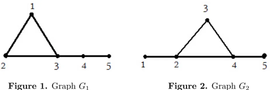
Example 2.1. Let’s take two connected graphs whose orders, edge numbers, vertex connectivity (), edge-connectivity (0) and average distance () value,
Figure 1. Graph 1 Figure 2. Graph 2
(1) = (2), 0(1) = 0(2) and (1) = (2) but 0(1) 0(2).
When we compare these two graph models we choose the one whose AED value is bigger. Since this means the communication is more stable in this graph than the other graph model.
Theorem 2.1. The average edge-distance takes its minimum value in star graph, 3 or 3and maximum value in complete graph.0 ≤ 0() ≤ (−2)(−3)4
Proof. In a 1star graph, 3and 3, any edge has common vertex with the
other edges. So = 0 in these graph 0= 0. In a complete graph it is
obvious that the number of the pair of edges and value is to be maximum. 0() = (−2)(−3)4 .
0(1) = 0(3) = 0(3) ≤ 0() ≤ 0()
Theorem 2.2. Let 1 and 2 be two connected graphs whose orders and
diameters are the same. If |(1)| |(2)| ⇒ 0(1) 0(2).
Proof. Since the diameters of these graphs are the same, the biggest elements in Edge-Distance Matrix of these two graphs are the same. The number of the pair edges examined is greater in the graph whose edge number is greater. And this cause value to increase. Since their sizes are the same |(1)|
|(2)| ⇒ 0(1) 0(2).
Theorem 2.3. If | (1)| = | (2)| and (1) (2) ⇒ 0(1)
0( 2).
Proof. Since | (1)| = | (2)| and (1) (2) then |(1)|
Theorem 2.4. Let 1 and 2 be two connected graphs whose orders and
diameters are the same. If 0(1) 0(2) ⇒ 0(1) 0(2).
Proof. Since 0(1) 0(2) then |(1)| |(2)|. From the Theorem 2.2
0(
1) 0(2).
Theorem 2.5. Let be a spanning sub graph of then 0() 0().
Proof. Number of the vertices of will remain the same as the graph itself. It is obvious that |()| |()|. From the Theorem 2.2 0() 0().
Theorem 2.6. Let’s take two connected graphs whose orders and diameters are the same. If (1) (2) ⇒ 0(1) 0(2).
Proof. Since (1) (2) then |(1)| |(2)|. From the Theorem 2.2
0(1) 0(2).
Theorem 2.7. Let 1 and 2 be two graphs of having the same order and
same diameter. If (1) (2) ⇒ 0(1) 0(2). Proof. || = 1 2 P ∈ () = 1
2() | | [5] . Since these graphs have the
same order if (1) (2) then |(1)| |(2)|. From the Theorem
2.2 0(1) 0(2).
3. Basic Results
1−1 1−1 are some basic graph types .In this section,
we give some results on .
Theorem 3.1. 0() =(−3)(−2)3 ≥ 3.
Proof. In path graph there are − 1 edges. The upper triangular matrix
of edge distance matrix of is obtained as follows. The element of first row
is0 1 2 ( − 3) ( − 3) is the distance between first and last edge since the definition of edge distance. Second row is 0 1 2 ( − 4). The other rows of EDM are obtained by the same way. Consequently
= 12 P−3 =1 ( + 1) = 16( − 3)( − 2)( − 1) Finally 0() = 2 = (−3)(−2) 3 ≥ 3 Theorem 3.2. 0() = ( (−2)2 4(−1) ≥ 4 and even (−3) 4 ≥ 3 and odd
Proof. In cycle graph there are n edges. For even n; since is regular
graph the element of any row of EDM except the diagonal element is occurred as following; 0 0 1 2 (−2 2 ) ( −2 2 ) − 1 ( −2 2 ) − 2 2 1. (the diameter of is (−22 ),n even). Finally = ⎡ ⎣2 (−2 2 )−1 X =1 + ( − 2 2 ) ⎤ ⎦ 1 2 = ( − 2)2 8 and 0( ) = µ 2 ¶ = ( − 2)2 4( − 1)
For odd n; similar way as above = " 2 −3 2 P =1 # 12 = (−3)(−1)8 and 0( ) =(−3)4 . Theorem 3.3. 0() =(−2)(−3)4 .
Proof. Any edge taken from has (2.(n-2)) edge-neighbors (due to the end
points of this edge) and µ
− 2 2
distinct edge. The edge-distance between any edge and its neighbor is 0 and the edge-distance between any edge and distinct edge in is 1. Finally
= µ 2 ¶ µ − 2 2 ¶ 1 2 and 0( ) = µ 2 ¶ = µ − 2 2 ¶ 1 2= (−2)(−3) 4 Theorem 3.4. 0( 1) = ( (−2)(+6) 4(+1) ≥ 4 and even 2+4 −13 4 ≥ 3 and odd
Proof. There exist 3 cases in a wheel graph to examine pair edge relations. These are the following,
(i)Edges in the outer cycle
In outer cycle there are n edges. From 3.2 for even n TED = (−2)8 2 and for odd n TED = (−3)(−1)8 .
(ii)Inside edges
The number of inside edges is n and any of them has common vertex with the others. So the TED = 0.
(iii)One edge from outer cycle and one from inside
Any edge from outer cycle has common vertex with two edges and has no com-mon vertex with (n-2) edges. The edge-distance between neighbor edges is 0.
The edge-distance between any edge from outer cycle and the distinct edge is 1. TED = n(n-2). So, = ( (−2)2 8 + ( − 2) ≥ 4 and even (−3)(−1) 8 + ( − 2) ≥ 3 and odd and finally 0(1) = µ + 1 2 ¶ = ( (−2)(+6) 4(+1) ≥ 4 and even 2+4−13 4(+1) ≥ 3 and odd Theorem 3.5. 0( 1) = 0.
Proof. In a star graph one vertex (which is in center) is adjacent to the others so every edges have one common vertex and = 0. 0(1) =
+ 1 2 = 0. Theorem 3.6. 0( ) = (+)(+(−1)(−1)−1) .
Proof. In a graph there are m.n edges. Any edge taken from has
(+−2) edge-neighbors (due to the end points of this edge) and ((−1)(−1)) distinct edge. The edge-distance between any edge and its neighbor is 0 and the edge-distance between any edge and distinct edge in is 1. Finally
= ( − 1)( − 1) 2 and 0( ) = µ + 2 ¶ = ( − 1)( − 1) ( + )( + − 1)
4. An Algorithm for Finding the Average Edge Distance of a Graph We give an algorithm whose complexity is (¯¯3¯¯) . This algorithm works
on the basis of adjacency matrix. By Floyd Marshall ((¯¯3¯¯)) [6] method distance matrix is calculated. Then the edge-distance matrix is calculated by the algorithm via distance matrix. values are calculated by this matrix. Finally 0 is calculated.
Step1. [ ] matrix of graph is given. Step2. [ ] distance matrix is constructed.
Step3. Each-distance is assigned to an element of an array.
Step4. [ ] edge-distance matrix of the graph is obtained from the distance matrix.
Step5. Each edge-distance is stored in an array.
Step6. (total edge-distance) is calculated by the use of edge-distance matrices.
Step7. Number of pair of vertices is calculated to find the all possible edges number.
Step8. 0 is calculated by the formula.
5. Conclusion
In this work we give a new measure on graphs. This measure is different from other measures. For example when we take two graphs having the same number of vertices and edges, we prefer the graph whose average edge-distance value is bigger. Since the pair edge relations is stronger in the graph having the higher average edge-distance value . This means if any failure happens in any link of the graph, there left much more links still working each other.
References
1. Arumungan,S., Velammal, S., (1998): Edge domination in graphs, Taiwanese Jour-nal of Mathematics, 2, 173-179.
2. Buckley,F., Harary F. (2001): Distance in Graphs, (New York, Addison Wesley). 3. Dankelmann, P.( 1997): Average distance and domination number, Discrete Applied Mathematics, 80, 21-35.
4. Dankelmann, P., Mukwembu, S., Swart, H.C., (2008): Average distance and edge connectivity I*, Siam J. Discrete Math, 22, 92-101.
5. Diestel, R. (2001): Graph Theory, (Verlag Heidelberg, Springer).
6. Jungnickel, D.(1999): Networks and Algorithms, (Verlag Heidelberg, Springer). 7. West,D.B. (2001): Introduction to Graph Theory, (U.S.A, Prentice Hall).