* Corresponding Author DOI: 10.37094/adyujsci.757642
Increasing the Efficiency of Percentile Parameter Estimation Method for Weibull
Distribution
Ülkü ERİŞOĞLU1, Murat ERİŞOĞLU2, Tayfun SERVİ3,*
1Necmettin Erbakan University, Faculty of Science, Department of Statistics, Konya, Turkey
[email protected], ORCID: 0000-0002-9826-3460
2Necmettin Erbakan University, Faculty of Science, Department of Statistics, Konya, Turkey
[email protected], ORCID: 0000-0002-4589-1383
3Adıyaman University, Faculty of Economics and Administrative Science of Science, Department of
Economics, Adıyaman, Turkey
[email protected], ORCID: 0000-0002-3173-327X
Received: 25.06.2020 Accepted: 10.08.2020 Published: 30.12.2020
Abstract
The Weibull distribution is one of the most widely used probability distributions in statistical applications. The percentile parameter estimation method is commonly used in parameter estimation of the two-parameter Weibull distribution in terms of easy computability and efficiency. The effectiveness of the percentile method depends on the selected percentile points and chosen empirical distribution function. In this study, the appropriate empirical distribution function and percentile points were determined to increase the efficiency of the percentile method for two-parameter Weibull distribution by simulation study.
Keywords: Weibull distribution; Percentile estimation; Empirical distribution function.
Weibull Dağılımı için Persentil Parametre Tahmin Yönteminin Etkinliğinin Artırılması Öz
Weibull dağılımı istatistiksel uygulamalarda en yaygın kullanılan olasılık dağılımlarından biridir. Persentil parametre tahmin yöntemi kolay hesaplanama ve etkinlik açısından iki parametreli Weibull dağılımının parametre tahmininde yaygın olarak kullanılır. Persentil yönteminin etkinliği seçilen persentil noktalara ve seçilen ampirik dağılım fonksiyonuna bağlıdır. Bu çalışmada, simülasyon çalışması ile iki parametreli Weibull dağılımı için persentil yönteminin etkinliğini artırmak amacıyla uygun ampirik dağılım fonksiyonu ve persentil noktaları belirlenmiştir.
Anahtar Kelimeler: Weibull dağılımı; Persentil tahmin; Ampirik dağılım fonksiyonu.
1. Introduction
The Weibull distribution is one of the widely used probability distributions which has many different applications and used for solving a variety of problems from many different disciplines. The Weibull distribution has many useful properties because its form is flexible to model different shapes. Weibull distribution has increasing, decreasing or stable failure rates depending on the values of the shape parameter. This feature has provided widespread use of the Weibull distribution. Because of its importance, many different estimation methods have been proposed for estimating parameters of Weibull distribution.
Percentile method is one of the commonly used methods for estimating the parameters of Weibull distribution and has some advantages unlike the other estimation methods in terms of ease compute and efficiency in parameter estimation [1].
The percentile method may be applied via two different approaches. The approach 1 is based on percentiles and is structurally similar to the traditional method of moments. The approach 2 is mainly obtained by minimizing the squared Euclidean distance between the sample percentile and population percentile [2].
The effectiveness of the percentile estimators depends on the selected percentile points and chosen empirical distribution function.
Dubey [3] proposed 17th and 97th percentiles for shape parameter and 40th and 82th percentiles for scale parameter. Seki and Yokoyama [4] suggested 31st and 63rd percentiles to estimate shape and scale parameters. Wang and Keats [5] proposed 15th and 63rd percentiles for parameter estimation of the Weibull distributions. Marks [6] stated that the best results were obtained with 10th and 90th percentiles for the shape and scale parameters.
In this study, we aimed to determine the appropriate empirical distribution and the percentile points to increase the effectiveness of the percentile estimators for the Weibull distribution. We used mean squared error (𝑀𝑆𝐸) and mean total error (𝑀𝑇𝐸) as performance criteria in the simulation study.
2. Weibull Distribution
The two-parameter Weibull distribution is specified by the probability density function (pdf) 𝑓(𝑥; 𝛼, 𝛽) =! ". # "/ !$% 𝑒$&"!' # , (1)
where 𝛼 > 0 and 𝛽 > 0 are the shape and scale parameters, respectively. The corresponding cumulative distribution function (cdf) and survival function (sf) are given as bellow:
𝐹(𝑥; 𝛼, 𝛽) = 1 − 𝑒$&!"' # , (2) 𝑆(𝑥; 𝛼, 𝛽) = 𝑒$&!"' # . (3)
Figure 1: The curves of the pdf, cdf, sf and hf of Weibull distribution for selected parameter values
The hazard function (hf) is given
which can be increase, decrease or constant depending on , 𝛼 > 1, 𝛼 < 1 or 𝛼 = 1, respectively. The curves of the pdf, cdf, sf and hf of Weibull distribution are shown in Fig. 1 for selected parameter values.
3. Percentile Method (PM)
The quantile function corresponding to Eqn. (1) is
𝑥( = 𝛽[−𝑙𝑛(1 − 𝑝)]% !⁄ . (5)
Percentile estimations of the Weibull distribution are calculated based on the obtained equations from selected two percentile points in the quantile function. The percentile estimators of the shape and scale parameters for Weibull distribution are respectively given by
𝛼> =*+[$*+(%$($)]$*+[$*+(%$(%)] *+0#&$1$*+0#&%1 , (6) 𝛽? = #&$ 0$*+(%$($)1$ #⁄' , (7)
where 𝑝% and 𝑝2 are selected two percentile points and 𝑥($ and 𝑥(% are observation values corresponding to 𝑝% and 𝑝2 , respectively. There are many approaches for selection of the 𝑝% and
𝑝2. For example, we can obtain an estimate for scale parameter by using one of these approaches like setting 𝑝% = 1 − 𝑒𝑥𝑝(−1) ≅ 0.632 (63.2th percentile point) into Eqn. (7). In this approach,
the percentile estimators for Weibull distribution are given
𝛽? = 𝑥%$3#( ($%), (8)
𝛼> = D*+[$*+(%$(%)]
*+0#&%1$*+0"51E, (9)
where 0 < 𝑥(%< 𝑥6.892 [7]. There are some suggestions for the optimum value of 𝑝2. Wang and Keats [5] showed by simulation that 0.15 would be the correct choice for 𝑝2. Seki and Yokoyama [8] suggested 𝑝2= 0.31.
The percentile based estimators for 𝛼 and 𝛽 of Weibull distribution according to approach 2 can be obtained by minimizing
∑ G𝑙𝑛𝑥(:)− 𝑙𝑛𝛽 −%
!𝑙𝑛H−𝑙𝑛 (1 − 𝐹J(:)KL 2 +
with respect to 𝛼 and 𝛽. The percentile estimators for 𝛼 and 𝛽 of the Weibull distribution are given by 𝛼> = <%$+= <>$+? , (11) 𝛽? = 𝑒𝑥𝑝 D%+.𝐶 −<!@/E, (12) where 𝐴 = ∑+ 𝑙𝑛 H− 𝑙𝑛H1 − 𝐹J(:)KK :;% , 𝐵 = ∑+:;%P𝑙𝑛 H− 𝑙𝑛H1 − 𝐹J(:)KKQ2, 𝐶 = ∑+:;%𝑙𝑛𝑥: and 𝐷 = ∑+ 𝑙𝑛𝑥:𝑙𝑛 H− 𝑙𝑛H1 − 𝐹J(:)KK :;% . 4. Simulation Study
In this study, we designed a simulation according to different sample size and different parameter values with the following purposes:
• To determine the best empirical distribution function respect to 𝑀𝑆𝐸 for approach 1 in the percentile method.
• To choose the best selected second percentile point 𝑝2 when setting 𝑝% = 1 − 𝑒𝑥𝑝(−1) ≅
0.632 for approach 1.
• To determine the best percentile pair among from several selected percentile pairs for approach 1 in the percentile estimation.
•
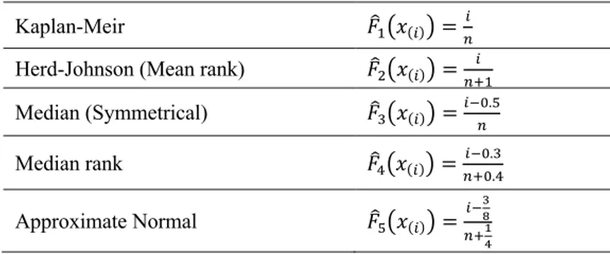
To determine the best empirical distribution function for the best successful estimation according to 𝑀𝑇𝐸 in the percentile estimation by approach 2.Table 1: The selected empirical distribution functions
Kaplan-Meir 𝐹"!#𝑥(#)% =%#
Herd-Johnson (Mean rank) 𝐹"&#𝑥(#)% =%'!#
Median (Symmetrical) 𝐹"(#𝑥(#)% =#)*.,%
Median rank 𝐹"-#𝑥(#)% =%'*.-#)*.(
Approximate Normal 𝐹",#𝑥(#)% = #)!" %'#$
Firstly, we examined fitness between empirical distribution functions and actual cumulative distribution function values of the Weibull distribution for approach 1 in the percentile estimation method. The selected EDFs are given in Table 1.
We used mean squared error (𝑀𝑆𝐸) in the comparison of the fitness between empirical distribution functions and actual cumulative distribution function values of Weibull distribution for the different parameter values and sample sizes.
𝑀𝑆𝐸A =%66666% ∑ ∑ BC(#(*);!,")$CF,(#(*))G % + + :;% %66666 H;% (13)
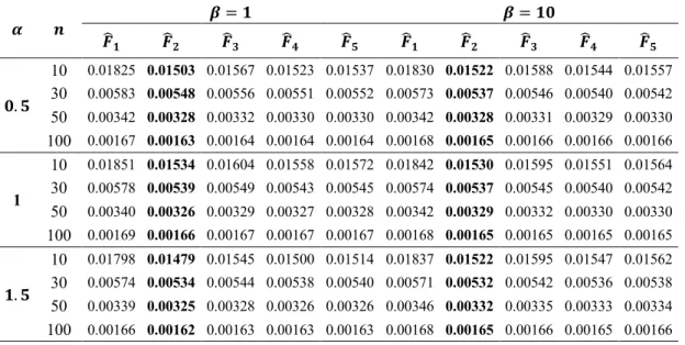
In the simulation study, 100000 random samples of sizes 10, 30, 50 and 100 were generated from Weibull distributions having 𝛼 = 0.5, 1, 1.5, 2, 3.4, 5 and 𝛽 = 1, 10. The comparisons of the empirical distribution functions respect to 𝑀𝑆𝐸 are given in Table 2.
In accordance with Table 2, the empirical distribution function that best matches the actual cumulative distribution function values of the Weibull distribution is Hard-Johnson's empirical distribution function for all the cases. Hard-Johnson’s function will be used as empirical distribution function in the determination of the best percentile pairs for the percentile estimations according to approach 1.
At this stage of the study, we will try to determine the best percentile point for the 𝑝%= 1 − 𝑒𝑥𝑝 (−1) ≅ 0.632 in the approach 1. For this, the 𝑀𝑆𝐸(𝛼>) values for all candidate points were determined with 0.01 increases from 0 to 0.63.
𝑀𝑆𝐸(𝛼>) =%6666% ∑%6666H;% (𝛼 − 𝛼>H)2 (14)
In the simulated study for the different parameter values and sample sizes, the percentile point with the smallest 𝑀𝑆𝐸(𝛼>) was determined, and the results are given in Table 3.
Table 2: The comparison of the EDFs according to MSE for different sample sizes and parameter values
𝜶 𝒏 𝜷 = 𝟏 𝜷 = 𝟏𝟎 𝑭-𝟏 𝑭-𝟐 𝑭-𝟑 𝑭-𝟒 𝑭-𝟓 𝑭-𝟏 𝑭-𝟐 𝑭-𝟑 𝑭-𝟒 𝑭-𝟓 𝟎. 𝟓 10 0.01825 0.01503 0.01567 0.01523 0.01537 0.01830 0.01522 0.01588 0.01544 0.01557 30 0.00583 0.00548 0.00556 0.00551 0.00552 0.00573 0.00537 0.00546 0.00540 0.00542 50 0.00342 0.00328 0.00332 0.00330 0.00330 0.00342 0.00328 0.00331 0.00329 0.00330 100 0.00167 0.00163 0.00164 0.00164 0.00164 0.00168 0.00165 0.00166 0.00166 0.00166 1 10 0.01851 0.01534 0.01604 0.01558 0.01572 0.01842 0.01530 0.01595 0.01551 0.01564 30 0.00578 0.00539 0.00549 0.00543 0.00545 0.00574 0.00537 0.00545 0.00540 0.00542 50 0.00340 0.00326 0.00329 0.00327 0.00328 0.00342 0.00329 0.00332 0.00330 0.00330 100 0.00169 0.00166 0.00167 0.00167 0.00167 0.00168 0.00165 0.00165 0.00165 0.00165 𝟏. 𝟓 10 0.01798 0.01479 0.01545 0.01500 0.01514 0.01837 0.01522 0.01595 0.01547 0.01562 30 0.00574 0.00534 0.00544 0.00538 0.00540 0.00571 0.00532 0.00542 0.00536 0.00538 50 0.00339 0.00325 0.00328 0.00326 0.00326 0.00346 0.00332 0.00335 0.00333 0.00334 100 0.00166 0.00162 0.00163 0.00163 0.00163 0.00168 0.00165 0.00166 0.00165 0.00166
Table 3: The percentile points values which have the smallest MSE(α5) for different sample sizes and parameter values Sample Size 𝒏 𝜷 = 𝟏 𝜷 = 𝟏𝟎 𝜶 𝜶 0.5 1 1.5 2 3.4 5 0.5 1 1.5 2 3.4 5 10 0.13 0.13 0.13 0.13 0.13 0.13 0.13 0.13 0.13 0.13 0.13 0.13 30 0.11 0.14 0.14 0.14 0.14 0.14 0.14 0.14 0.14 0.14 0.14 0.14 50 0.12 0.12 0.12 0.14 0.10 0.12 0.12 0.10 0.12 0.14 0.10 0.14 100 0.11 0.12 0.11 0.12 0.12 0.13 0.14 0.13 0.12 0.13 0.13 0.12 According to Table 3, the most suitable percentile points is found ranges 0.10 to 0.14 for the 𝑝%≅ 0.632 in the approach 1. The best percentile point was 0.13 with respect to 𝑀𝑆𝐸(𝛼>) in the shape parameter estimation of the Weibull distribution by this approach when the small sample size is 𝑛 = 10.
Here, the best percentile pair will be determined from the selected percentile pairs in the percentile estimation by approach 1 of the Weibull distribution parameters. The comparison is based on 𝑀𝑇𝐸 criterion defined by
𝑀𝑇𝐸 = % %6666∑ U. !@-$! ! / 2 + ."5-$" " / 2 W . %6666 H;% (15)
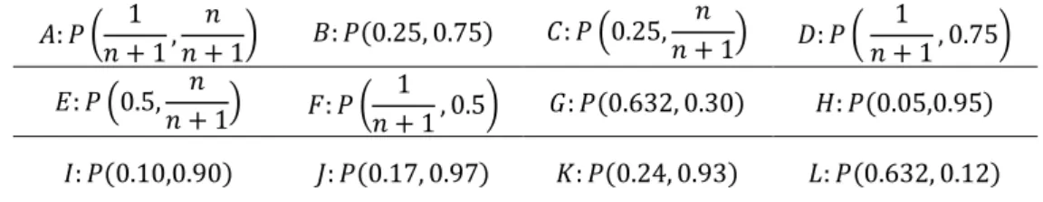
In this study, the selected percentile pairs are denoted in Table 4.
Table 4: The selected pairs of percentage point 𝐴: 𝑃 : 1 𝑛 + 1, 𝑛 𝑛 + 1? 𝐵: 𝑃(0.25, 0.75) 𝐶: 𝑃 F0.25, 𝑛 𝑛 + 1G 𝐷: 𝑃 : 1 𝑛 + 1, 0.75? 𝐸: 𝑃 F0.5, 𝑛 𝑛 + 1G 𝐹: 𝑃 : 1 𝑛 + 1, 0.5? 𝐺: 𝑃(0.632, 0.30) 𝐻: 𝑃(0.05,0.95) 𝐼: 𝑃(0.10,0.90) 𝐽: 𝑃(0.17, 0.97) 𝐾: 𝑃(0.24, 0.93) 𝐿: 𝑃(0.632, 0.12) 𝟐 10 0.01822 0.01512 0.01577 0.01533 0.01546 0.01829 0.01508 0.01573 0.01529 0.01542 30 0.00577 0.00543 0.00551 0.00546 0.00547 0.00564 0.00530 0.00539 0.00533 0.00535 50 0.00337 0.00324 0.00327 0.00325 0.00326 0.00342 0.00331 0.00334 0.00332 0.00333 100 0.00167 0.00164 0.00165 0.00165 0.00165 0.00169 0.00166 0.00166 0.00166 0.00166 𝟑. 𝟒 10 0.01833 0.01530 0.01598 0.01553 0.01567 0.01829 0.01502 0.01573 0.01526 0.01541 30 0.00578 0.00540 0.00549 0.00543 0.00545 0.00578 0.00541 0.00549 0.00543 0.00545 50 0.00344 0.00331 0.00335 0.00333 0.00333 0.00340 0.00327 0.00330 0.00328 0.00329 100 0.00167 0.00164 0.00164 0.00164 0.00164 0.00167 0.00163 0.00164 0.00163 0.00163 𝟓 10 0.01833 0.01520 0.01589 0.01543 0.01557 0.01859 0.01529 0.01599 0.01553 0.01567 30 0.00570 0.00536 0.00545 0.00539 0.00541 0.00573 0.00535 0.00544 0.00538 0.00540 50 0.00346 0.00332 0.00335 0.00333 0.00334 0.00340 0.00327 0.00330 0.00328 0.00329 100 0.00168 0.00165 0.00166 0.00165 0.00165 0.00170 0.00167 0.00168 0.00167 0.00167
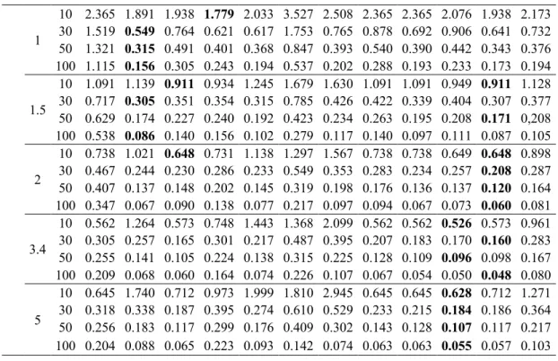
In the simulation study, the obtained 𝑀𝑇𝐸 values for different parameter values and sample sizes are given in Table 5.
According to Table 5, in case of the scale parameter is equal 1, 𝐽 and 𝐾 percentile pairs point are more successful than other percentile pairs for ≥ 1 . The 𝐵 percentile pair is more successful than other pairs for 𝛼 < 1 and 𝛽 = 1. In case of the scale parameter is set as 𝛽 = 10, 𝐵 percentile pair is more successful than other percentile pairs for 𝛼 ≤ 1 . The 𝐾 percentile pair is more successful than other pairs for 𝛼 = 2 and 𝛽 = 10. In addition, J percentile pair showed more performance than other pairs for 𝛼 = 5 and 𝛽 = 10.
Finally, we performed a simulation study to investigate the performance of empirical distribution functions in the percentile estimates for parameters of the Weibull distribution by approach 2. The comparison results of the empirical distribution functions according to 𝑀𝑇𝐸 for different sample sizes and parameter values in the approach 2 are given in Table 6.
Table 5: The comparison results of the selected percentage points according to 𝑀𝑇𝐸
𝜷 𝜶 𝒏 A B C D E F G H I J K L 1 0.5 10 1.725 1.201 1.376 1.126 1.405 3.677 1.617 1.725 1.725 1.538 1.376 1.679 30 0.899 0.265 0.418 0.288 0.320 1.478 0.394 0.457 0.348 0.544 0.328 0.408 50 0.689 0.150 0.262 0.178 0.182 0.530 0.176 0.260 0.186 0.226 0.165 0.177 100 0.553 0.070 0.148 0.104 0.091 0.308 0.090 0.131 0.086 0.108 0.078 0.094 1 10 0.341 0.462 0.315 0.336 0.540 0.640 0.428 0.341 0.341 0.312 0.315 0.552 30 0.201 0.109 0.104 0.132 0.106 0.280 0.132 0.124 0.103 0.119 0.092 0.160 50 0.167 0.064 0.068 0.093 0.066 0.155 0.075 0.077 0.061 0.062 0.054 0.075 100 0.143 0.031 0.040 0.065 0.036 0.107 0.038 0.042 0.030 0.032 0.027 0.046 1.5 10 0.264 0.523 0.271 0.332 0.620 0.586 0.424 0.264 0.264 0.250 0.271 0.610 30 0.143 0.111 0.077 0.139 0.098 0.237 0.126 0.096 0.084 0.081 0.073 0.168 50 0.117 0.065 0.050 0.101 0.062 0.146 0.075 0.059 0.051 0.046 0.045 0.076 100 0.098 0.030 0.029 0.076 0.034 0.107 0.037 0.033 0.025 0.024 0.023 0.049 2 10 0.279 0.647 0.304 0.391 0.773 0.685 0.503 0.279 0.279 0.270 0.304 0.752 30 0.142 0.131 0.079 0.167 0.112 0.266 0.147 0.099 0.090 0.079 0.078 0.203 50 0.113 0.076 0.050 0.123 0.071 0.170 0.088 0.061 0.055 0.047 0.049 0.089 100 0.093 0.035 0.029 0.094 0.039 0.127 0.043 0.034 0.028 0.024 0.024 0.059 3.4 10 0.405 1.052 0.464 0.615 1.262 1.079 0.798 0.405 0.405 0.401 0.464 1.220 30 0.191 0.207 0.112 0.264 0.172 0.408 0.230 0.141 0.131 0.107 0.113 0.324 50 0.149 0.120 0.070 0.196 0.110 0.267 0.138 0.087 0.080 0.065 0.072 0.140 100 0.118 0.055 0.040 0.152 0.061 0.201 0.067 0.047 0.041 0.033 0.036 0.094 5 10 0.576 1.534 0.668 0.891 1.843 1.566 1.159 0.576 0.576 0.575 0.668 1.780 30 0.268 0.300 0.158 0.384 0.249 0.590 0.333 0.200 0.188 0.150 0.161 0.472 50 0.208 0.174 0.099 0.285 0.159 0.387 0.201 0.123 0.114 0.092 0.102 0.203 100 0.163 0.080 0.056 0.222 0.088 0.292 0.097 0.067 0.058 0.046 0.051 0.137 10 0.5 10 17.08 10.58 13.31 10.63 11.52 34.29 14.61 17.08 17.08 14.93 13.31 14.45 30 8.534 2.384 4.152 2.538 2.950 13.81 3.678 4.403 3.298 5.195 3.177 3.661 50 6.913 1.280 2.456 1.468 1.617 4.867 1.534 2.410 1.679 2.083 1.498 1.525 100 5.311 0.602 1.454 0.796 0.804 2.826 0.779 1.204 0.781 1.018 0.707 0.775
1 10 2.365 1.891 1.938 1.779 2.033 3.527 2.508 2.365 2.365 2.076 1.938 2.173 30 1.519 0.549 0.764 0.621 0.617 1.753 0.765 0.878 0.692 0.906 0.641 0.732 50 1.321 0.315 0.491 0.401 0.368 0.847 0.393 0.540 0.390 0.442 0.343 0.376 100 1.115 0.156 0.305 0.243 0.194 0.537 0.202 0.288 0.193 0.233 0.173 0.194 1.5 10 1.091 1.139 0.911 0.934 1.245 1.679 1.630 1.091 1.091 0.949 0.911 1.128 30 0.717 0.305 0.351 0.354 0.315 0.785 0.426 0.422 0.339 0.404 0.307 0.377 50 0.629 0.174 0.227 0.240 0.192 0.423 0.234 0.263 0.195 0.208 0.171 0,208 100 0.538 0.086 0.140 0.156 0.102 0.279 0.117 0.140 0.097 0.111 0.087 0.105 2 10 0.738 1.021 0.648 0.731 1.138 1.297 1.567 0.738 0.738 0.649 0.648 0.898 30 0.467 0.244 0.230 0.286 0.233 0.549 0.353 0.283 0.234 0.257 0.208 0.287 50 0.407 0.137 0.148 0.202 0.145 0.319 0.198 0.176 0.136 0.137 0.120 0.164 100 0.347 0.067 0.090 0.138 0.077 0.217 0.097 0.094 0.067 0.073 0.060 0.081 3.4 10 0.562 1.264 0.573 0.748 1.443 1.368 2.099 0.562 0.562 0.526 0.573 0.961 30 0.305 0.257 0.165 0.301 0.217 0.487 0.395 0.207 0.183 0.170 0.160 0.283 50 0.255 0.141 0.105 0.224 0.138 0.315 0.225 0.128 0.109 0.096 0.098 0.167 100 0.209 0.068 0.060 0.164 0.074 0.226 0.107 0.067 0.054 0.050 0.048 0.080 5 10 0.645 1.740 0.712 0.973 1.999 1.810 2.945 0.645 0.645 0.628 0.712 1.271 30 0.318 0.338 0.187 0.395 0.274 0.610 0.529 0.233 0.215 0.184 0.186 0.364 50 0.256 0.183 0.117 0.299 0.176 0.409 0.302 0.143 0.128 0.107 0.117 0.217 100 0.204 0.088 0.065 0.223 0.093 0.142 0.074 0.063 0.063 0.055 0.057 0.103 Table 6: The comparison results of the empirical distribution functions according to 𝑀𝑇𝐸 for different sample sizes and parameter values in the approach 2
𝜶 𝒏 𝜷 = 𝟏 𝜷 = 𝟏𝟎 𝑭 -𝟏 𝑭-𝟐 𝑭-𝟑 𝑭-𝟒 𝑭-𝟓 𝑭-𝟏 𝑭-𝟐 𝑭-𝟑 𝑭-𝟒 𝑭-𝟓 0.5 10 0.6209 1.2054 0.8843 0.8976 0.9490 5.6093 11.584 8.2614 7.0162 8.9809 30 0.1872 0.2579 0.2137 0.2210 0.2236 1.6950 2.4080 1.9811 1.8365 2.0847 50 0.1157 0.1439 0.1238 0.1278 0.1284 1.0498 1.3319 1.1438 1.0858 1.1906 100 0.0563 0.0647 0.0579 0.0595 0.0594 0.5066 0.5902 0.5293 0.5127 0.5445 1 10 0.2533 0.2632 0.2600 0.2384 0.2500 1.3328 1.6937 1.4358 1.1833 1.4813 30 0.0791 0.0840 0.0755 0.0751 0.0757 0.4369 0.4981 0.4433 0.4030 0.4545 50 0.0485 0.0511 0.0457 0.0461 0.0461 0.2704 0.2972 0.2696 0.2523 0.2753 100 0.0247 0.0258 0.0232 0.0236 0.0235 0.1341 0.1440 0.1332 0.1277 0.1354 1.5 10 0.2562 0.2186 0.2479 0.2147 0.2254 0.7622 0.7778 0.7332 0.6168 0.7262 30 0.0770 0.0762 0.0696 0.0683 0.0684 0.2385 0.2494 0.2277 0.2120 0.2300 50 0.0468 0.0473 0.0421 0.0422 0.0420 0.1458 0.1518 0.1391 0.1330 0.1407 100 0.0242 0.0247 0.0218 0.0222 0.0220 0.0728 0.0758 0.0700 0.0683 0.0709 2 10 0.2998 0.2418 0.2884 0.2444 0.2567 0.5974 0.5413 0.5556 0.4810 0.5305 30 0.0889 0.0864 0.0791 0.0773 0.0772 0.1810 0.1815 0.1671 0.1610 0.1668 50 0.0540 0.0540 0.0477 0.0479 0.0474 0.1099 0.1117 0.1018 0.1004 0.1023 100 0.0281 0.0285 0.0249 0.0254 0.0251 0.0555 0.0569 0.0519 0.0519 0.0524 3.4 10 0.4657 0.3656 0.4500 0.3761 0.3950 0.5763 0.4645 0.5415 0.4838 0.4879 30 0.1374 0.1326 0.1212 0.1182 0.1177 0.1700 0.1646 0.1514 0.1538 0.1483 50 0.0834 0.0831 0.0730 0.0732 0.0724 0.1030 0.1026 0.0916 0.0949 0.0911
100 0.0436 0.0442 0.0383 0.0391 0.0385 0.0531 0.0539 0.0476 0.0497 0.0479 5 10 0.6727 0.5264 0.6515 0.5433 0.5705 0.7258 0.5715 0.6938 0.6165 0.6133 30 0.1984 0.1913 0.1749 0.1705 0.1697 0.2137 0.2060 0.1888 0.1932 0.1838 50 0.1205 0.1200 0.1053 0.1056 0.1043 0.1296 0.1289 0.1138 0.1189 0.1129 100 0.0631 0.0639 0.0552 0.0565 0.0556 0.0675 0.0683 0.0595 0.0627 0.0599
In the large sample sizes (𝑛 = 50 and 100), the difference between 𝑀𝑇𝐸 values of the empirical distribution functions was not significant according to Table 6. In case of the shape parameter is set as 𝛼 = 0.5, Kaplan-Meir’s empirical distribution function has lower 𝑀𝑇𝐸 value than other empirical distribution functions for 𝛽 = 1 and 10.
5. Conclusion
In this paper, we aimed at improving the effectiveness of the percentile method for two parameter Weibull distribution. Based on simulation study, the empirical distribution function that best fits the actual Weibull cumulative distribution function is the empirical distribution function of Hard Johnson according to 𝑀𝑆𝐸. In conclusion, the most suitable percentage points ranged from 0.10 to 0.14 when 𝑝% value was nearly set as 0.632 in the percentile method by approach 1. In general, (0.17, 0.97) and (0.24, 0.93) percentile pairs were the best successful percentile pairs for 𝛼 ≥ 1. In case of the 𝛼 < 1, (0.25, 0.75) percentile pair was more successful than other percentile pairs. Also, median (symmetrical) empirical distribution function has been more successful in case of large sample size (𝑛 = 100) for percentile method by approach 2.
References
[1] Castillo, E., Hadi, A.S., A method for estimating parameters and quantiles of
distributions of continuous random variables, Computational Statistics & Data Analysis, 20(4),
421-439, 1995.
[2] Erisoğlu, U., Erisoğlu, M., Percentile estimators for two-component mixture
distribution models, Iranian Journal of Science and Technology, Transactions A: Science, 43(2),
601-619, 2019.
[3] Dubey, S.D., Some percentile estimators for Weibull parameters, Technometrics, 9(1), 119-129, 1967.
[4] Seki, T., Yokoyama, S., Simple and robust estimation of the Weibull
parameters, Microelectronics Reliability, 33(1), 45-52, 1993.
[5] Wang, F.K., Keats, J.B., Improved percentile estimation for the two-parameter Weibull
distribution, Microelectronics Reliability, 35(6), 883-892, 1995.
[6] Marks, N.B., Estimation of Weibull parameters from common percentiles, Journal of Applied Statistics, 32(1), 17-24, 2005.
[7] Teimouri, M., Hoseini, S.M., Nadarajah, S., Comparison of estimation methods for the
Weibull distribution, Statistics, 47(1), 93-109, 2013.
[8] Seki, T., Yokoyama, S., Robust parameter-estimation using the bootstrap method for