Disaggregation of annual to monthly streamflow: a case study of Kızılırmak Basin (Turkey)

(1)

Research Article

Disaggregation of Annual to Monthly Streamflow: A Case

Study of K

JzJlJrmak Basin (Turkey)

Shatha H. D. Al-Zakar,

1,2

N. Farlak,

3

and Omar M. A. Mahmood Agha

1,2

1_{Department of Dams and Water Resources Engineering, Mosul University, Mosul, Iraq} 2_{Department of civil Engineering, Gaziantep University, Gaziantep, Turkey}

3_{Department of Civil Engineering, Karamanoglu Mehmetbey University, Karaman, Turkey}

Correspondence should be addressed to Shatha H. D. Al-Zakar; [email protected]

Received 28 November 2016; Revised 12 January 2017; Accepted 24 January 2017; Published 23 February 2017 Academic Editor: Francesco Viola

Copyright © 2017 Shatha H. D. Al-Zakar et al. This is an open access article distributed under the Creative Commons Attribution License, which permits unrestricted use, distribution, and reproduction in any medium, provided the original work is properly cited.

This study utilizes a recent nonparametric disaggregation𝐾-nearest neighbor (𝐾NN) model, to resample monthly flows depending on annual flows at different sites. Both temporal and spatial approaches will be followed in this model while preserving the distributional statistics of the observed data. This model assumes that a set of aggregated annual streamflows at a key station is available and desired for disaggregation to a corresponding series of streamflow at key station (temporal disaggregation) as well as at tributary stations (spatial disaggregation). The model is applied to the annual streamflow data of particular stations in the Kızılırmak Basin, which is exposed to drought periods during the years (1970–1974 and 1994-1995). The aim of this study is to find the possibilities of using the nonparametric approaches as generators of monthly flows, with emphasis on the ability to reproduce the statistics related to drought and storage analysis for the selected stations in Turkey. The results show that the spatial disaggregation approach has the ability to reproduce the historical data better than the temporal approach for the tested sites and provides a variety of generated monthly sequence flows that can then be utilized to analyze the performance of the water resources planning system.

1. Introduction

Streamflow simulation is an important component in the analysis of water resource management, flood, drought, and reservoir operation. Water resources planning and man-agement depend mostly on the observed streamflow data. The lack of streamflow data is an obstacle to suitable water resources management, especially in the developing coun-tries. Additionally, the lack of fine temporal resolution data (e.g., daily) for detailed hydrological model represents another problem. Streamflow simulation processes have ear-lier been performed utilizing linear autoregressive moving average (ARMA) models for annual data and parametric autoregressive (PAR) for seasonal data. These models joined with some assumptions like a probability distribution apply-ing to the historical flow. Pumo et al. [1] developed a model to estimate monthly runoff depending on many variables, like precipitation, temperature, and exploiting the autocorrelation with runoff at the previous month. The model reproduced

the observed hydrological time series at both monthly and coarser time resolutions. Among the available stochastic generation models, the disaggregation method is proposed to overcome the problem of data limitation. Through this method, streamflow can be disaggregated into lower-level scales, either temporally or spatially. While the only one streamflow data set observed at the key station can be used in temporal disaggregation method, we can include the data of periphery stations into the simulation procedure in spatial disaggregation method.

There are two main disaggregation methods: parametric and nonparametric. Unlike the nonparametric approaches, parametric approaches require linearity and statistical dis-tribution assumptions. The first parametric approach was proposed by [2] to disaggregate the annual to seasonal streamflows using a linear autoregressive (AR) model for a single site. Although their approach is accepted as a pioneer disaggregation model, it has two disadvantages: (1) the moments being preserved are not consistent; (2) the number

(2)

of parameters is large [3]. The basic approach was improved by adding a column matrix containing seasonal values of the previous year and one more parameter matrix [4]. The model required an excessive number of parameters to be estimated. So, a condensed model was introduced for the temporal disaggregation model to reduce the number of parameters required drastically [5]. The autoregressive moving average (ARMA) and typical PAR(1) models were also utilized to modify and improve the basic model [6]. A periodic disaggregation method was proposed by [7] for disaggregation into subseasonal flows from seasonal flows generated from a periodic autoregressive (PAR) scheme of any order. The model also shows the ability to preserve the first and second moments of the decade (10-day) flows generated from monthly flows. Indeed, some aforementioned approaches have concentrated on the temporal disaggrega-tion of annual to seasonal or seasonal to subseasonal flows and fit in the transformed space. However, the summation of disaggregation flows may not ensure preserving the historical statistics when the results are back transformed to the original flow domain. So, a stepwise disaggregation approach was suggested by [8] to solve the inconsistency problem of the additive disaggregation approaches. Some studies demonstrated that nonparametric disaggregation models can overcome the drawbacks of the parametric ones [9–11]. The nonparametric approach was utilized by [9] including kernel density estimation approach. Then, this model was

improved by [10] using𝐾-nearest neighbor (𝐾-NN) method

to resample monthly flows depending on an annual flow value in a temporal disaggregation or multiple upstream sites based on a downstream site for a spatial disaggregation. This model shows the ability to capture all statistical distributional

properties of monthly flows at all sites. Meanwhile, the𝐾NN

approach presented by [11] was effective to resample daily flows at multisite from a single annual flow value. The model is flexible for disaggregation of annual to any different time scales and preserves the historical statistics very well. The nearest neighbor approach was utilized also in nonparametric approach by [12] to disaggregate seasonal flow to daily flow which includes a two stepwise: from season to monthly disaggregation followed by monthly to daily disaggregation to overcome the weakness of the stepwise procedure presented in parametric approach which is unable to preserve the historical correlation between flows of the first day of the month and last day of a previous month. The software package (stepwise) of model [8] was developed and extended by [13] to be implemented for the multivariate stochastic emulation and disaggregation of monthly hydrological time series to daily series that preserves the characteristics of annual, monthly, and daily historical data. With some nonparametric methods, the values not seen in the historical data cannot be

generated. To treat this problem, a modified𝐾-NN bootstrap

was suggested [14]. This approach is found to offer better performance in capturing the features of historical data when compared to both a periodic autoregressive parametric approach and a nonparametric index sequential method. Additionally, another method was suggested to disaggregate generated annual streamflow data into monthly streamflow series using three approaches with different criteria to set

the classes of fragments and to select the fragments [15]. For disaggregation monthly streamflows to a daily flow, a method based on an autoregressive model was presented by [16], and they obtained a good result for reproducing duration curves and the hydrographs of the streamflow.

Given the past researches as described above, it is clear that there is a need for a robust, simple, and parsimonious approach for space-time streamflow disaggregation that can capture any arbitrary features exhibited by the data and applied easily to regulated and unregulated waterways. To this end, we adopted a nonparametric disaggregation model

via𝐾-nearest-neighbor approach to resample the monthly

flow in both temporal and spatial disaggregation because the

method is parsimonious, as only the parameter𝐾 (number

of nearest neighbors to be used in resampling) is estimated. The model is utilized to generate monthly streamflow series starting from historical annual data at three stations on the Kızılırmak Basin which, in turn, may be used to manage the water resources system in this region.

2. Methodology

The𝐾-NN resample approach was firstly utilized by [17] to

develop a nonparametric disaggregation method. They man-aged to alleviate the drawbacks of the classical parametric and nonparametric methods based on kernel density estimation.

However, the𝐾-NN approach generates only historical values

as it is a resampling technique. The model developed by [11] indicated that aforesaid models are not performing well for disaggregation to daily time scales. Their method is based

on conditional probability distribution function,𝑓(𝑋_𝑡/𝑝_𝑡),

where𝑋_𝑡is a matrix of flows that sum the vector of annual

aggregate flows to be disaggregated, and𝑝_𝑡is the vector of

daily proportions, whose elements sum to unity. Their model can be used to disaggregate the annual data to different time scales. The steps of disaggregation annual historical data to monthly data temporally in a single site are summarized as follows. The detailed procedure of the methodology can be found in Nowak et al. [11].

(1) Historical monthly streamflow data at any year are transformed to a proportion of the total annual flow to

obtain [𝑃_𝑦1(= streamflow value observed on January

in an apparent year/total annual flow for an apparent

year), . . . , 𝑃_𝑦12] of that year; the same procedure is

repeated for all months in the years to obtain a

proportion vector matrix,𝑃_𝑦, with dimensions𝑛 × 13

(first column represents the historical years and the other columns represent the monthly flows) where 𝑛 is sample size. The summation of each row except the first column in the matrix should be unity. Then the historical annual flow data are written as a matrix

form,𝑧, with dimensions 𝑛 × 2.

(2) Assume that𝑍 is the annual flow of any year required

to be disaggregated. 𝐾 nearest neighbors of 𝑍 are

selected from the historical annual flow (𝑧). The

number of neighbors, 𝐾, is calculated from the

heuristic scheme as (𝐾 = 𝑛0.5_{) which is a well-known}

(3)

Station name Longitude Latitude Historical duration Sample size 1528-Salur 34∘39󸀠02󸀠󸀠 40∘39󸀠05󸀠󸀠 1964–1996 32 1517-Sefaatli 34∘44󸀠51󸀠󸀠 39∘30󸀠14󸀠󸀠 1953–2000 47 1541-Cadirhoyuk 34∘07󸀠09󸀠󸀠 40∘18󸀠31󸀠󸀠 1981–2000 19 1503-Yahsihan 33∘28󸀠54󸀠󸀠 39∘50󸀠36󸀠󸀠 1939–2000 61 1501-Yamulu 35∘15󸀠31󸀠󸀠 38∘53󸀠25󸀠󸀠 1939–2000 61

Figure 1: Gauges station schematic: (1) EIE1528; (2) EIE1541; (3) EIE1517; (4) EIE 1503; (5) EIE1501.

each 𝐾 nearest data by using the weight function,

𝑊(𝑖), as

𝑊 (𝑖) = 1

𝑖 ∗ (∑𝐾_𝑖=1(1/𝑖)), where 𝑖 = 1, 2, . . . , 𝐾. (1)

The weight function provides larger weight to the nearest neighbors and less weight to the farthest neighbors.

(3) One of the 𝐾-nearest neighbors (one of historical

years) is chosen depending on the weight function from (1). The proportion vector corresponding to

the chosen year, (𝑃_𝑦), is multiplied by the annual

streamflow (𝑍) to obtain the monthly streamflow vector (𝑑), which is given as

𝑑 = 𝑍 ∗ 𝑃_𝑦. (2)

(4) Steps (2) and (3) are repeated to generate all ensem-bles of monthly streamflows.

For spatial disaggregation, the procedure takes another

dimension. The matrix𝑃 (13 × 𝑛) will be arranged as (13 ×

𝑛 × 𝑠), where 𝑠 represents the number of sites needed to

be disaggregated. Therefore, the proportion vector 𝑃_𝑦 will

become a matrix of the dimension (13 × 𝑠).

3. Study Area

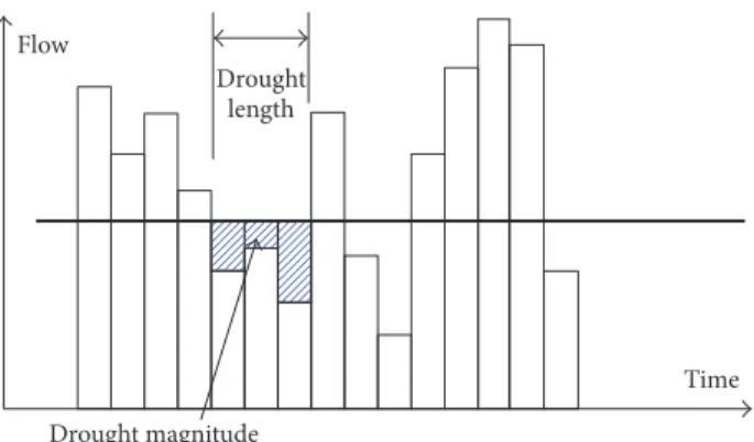
Data of the study were selected from three streamflow gauging stations located along the Kızılırmak River in Turkey since they have the longest length of historical data. Indeed,

Kızılırmak River is the longest river in Turkey with a length

of 1355 km and the basin size of 122,277 km2 [19]. The gauge

stations are Salur (EIE 1528) and Yahsihan (EIE 1503) which are located on the main river and Cadirhoyuk (EIE 1541) located on the biggest tributary (Delice River) of the main river as shown in Figure 1. Site information, including latitude, longitude, elevation, and observation period, is listed in Table 1. Historical monthly streamflow data were provided by the General Directorate of State Hydraulic Works (DSI). As shown in Figure 1, EIE 1503 and EIE 1528 stations are located downstream of the existing dams (Hirfanlı, Kesikk¨opr¨u Dam, and Kapulukaya). Since the observed streamflow data of the two stations have been influenced by the existing dams, unaffected streamflows of these two stations should be obtained. EIE 1501 station, located upstream of the dams, and EIE 1541 station, located on the tributary, were used as a reference to obtain the natural streamflow values (unaffected form) of the stations by obtaining the correlation coefficient between the monthly observed data of these stations before the construction of the dams. Furthermore, data of EIE 1517 streamflow gauging station were used to extend the data of observation duration of EIE1541 station. The measures of

goodness of fits (𝑅2) which are explained by EIE 1503 with

EIE 1501, EIE 1541 with EIE 1517, and EIE 1528 with EIE 1503 + EIE 1541 were 0.96, 0.86, and 0.88, respectively. These relationships are reasonably good to obtain the natural data by using the regression equation.

4. Results and Discussion

The statistics include monthly mean, variance, skewness coefficient, minimum and maximum discharge, and lag-1

(4)

Flow

Drought length

Drought magnitude

Time

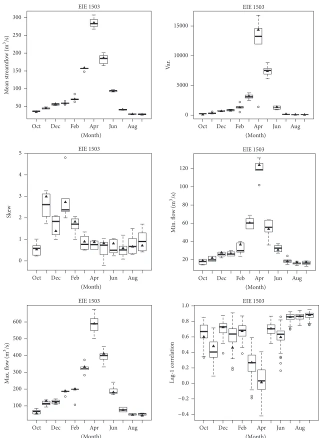
Figure 2: Definition of drought statistics.

autocorrelation coefficient of flow for the three stations. Statistics were calculated from 100 simulated traces; each trace consists of 37 years (the same length of annual observed streamflow data at each station), using both temporal and spatial nonparametric approaches for comparison. In addi-tion, drought analysis, including maximum length and mag-nitude, and storage capacity are also calculated from monthly simulation values to evaluate the performances of the two approaches. These statistics are displayed as boxplots. A box in the boxplots indicates the interquartile range of simula-tions and whiskers, ranging between 5th and 95th percentile confidence bounds. The horizontal line in the box represents the median of simulated values, while the dots represented the outside values in this range. The historical statistics are denoted as a triangle. Performance of any statistic is considered good when the historic statistic value falls within the range of the box.

The mean discharge from the 100 generated flow series is taken as a threshold in order to calculate the drought statistics. So, each period of one or more consecutive months with flow below the mean values is defined as a drought event and the length of each drought event is the duration of the period with flow below the mean discharge while the magnitude is the deficit of the total volume carried by each event with respect to the mean total volume relative to that length (i.e., product of the mean discharge by the length of drought) as shown in Figure 2. In general, some drought lengths are obtained in a time series in order to select demand level and model size. The drought characteristics of the model are computed and presented as boxplots to be compared with that obtained from the historical series [3].

The reservoir storage capacity is calculated by applying the sequent peak method [20]. Some release values are taken as a threshold release ranging between 10% and 90% of the mean monthly discharge. To evaluate the storage

capacity, the monthly mean storage (𝐴_𝑔) and the standard

deviation[𝜎(𝐴_𝑔)] for 100 generated time series are estimated

to find the range limits of storage capacities which can

be computed from [𝐴_𝑔 − 𝐾 ∗ 𝜎(𝐴_𝑔); 𝐴_𝑔 + 𝐾 ∗ 𝜎(𝐴_𝑔)]

where 𝐾 can equal 1.0, 1.5, or 2.0. 𝐾 could be taken as

1.96 for 5% significance level [3, 21]. The monthly storage

capacities of simulated data were compared with historical ones.

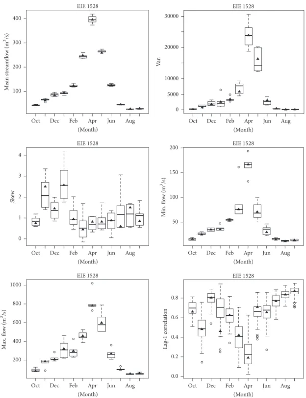
4.1. Temporal Disaggregation Results. The monthly basic statistics from the temporal disaggregation approach along the observed results were presented in Figure 3 (station EIE1503), Figure 4 (station 1541), and Figure 5 (station 1528). It can be seen from the figures that the model reproduces the mean value statistic well in each station. The tighten boxplots indicate that the 100 simulations have a high level of agreement with each other as well as with the historical data. In addition, the mean of historical streamflow data was nearly the same as the median of the simulated data for each month and stations. Boxplots of the variance and skewness coefficient statistics also show that the model is efficient in reproducing the historical data. Furthermore, the variance and skewness values of the historical data were within the boxplot for each month. Extreme behaviors of the simulated streamflow were inspected since they are of primary importance in analyzing reservoir operations and river basin management policies through minimum and maximum results. Also, the results of the minimum and maximum monthly values were reasonably well simulated in all stations. Backward lag-1 correlations are also well captured in all months, which indicated that the generated flows have factual continuity. It can be seen that only the last month of the year and the first month of the next year (December-January) are not captured well in all stations.

The drought analysis was applied to monthly inflow values obtained from the approach. It includes the maximum length period and maximum magnitude of drought. Accord-ing to Figure 6, the simulated maximum length of drought periods tends to be good at station EIE1541 and over and lower estimated at EIE1528 and EIE1503 stations, respectively (i.e., the simulated maximum length of drought periods). For the maximum magnitude of drought (Figure 6(b)), the results of the boxplots show that the model is unable to reproduce efficiently at EIE1541 station and that the historical statistic is near the edge of the box at EIE1503 and EIE1528 stations.

(5)

EIE 1503 EIE 1503 EIE 1503 EIE 1503 EIE 1503 EIE 1503 Jun Feb

Oct Dec Apr Aug

(Month)

Jun Feb

Oct Dec Apr Aug

(Month) 100 200 300 400 500 600 M ax. flo w ( m 3 /s) Jun Feb

Oct Dec Apr Aug

(Month) 0 1 2 Ske w 3 4 5 20 40 60 80 100 120 M in. flo w ( m 3/s) Jun Feb

Oct Dec Apr Aug

(Month) −0.4 −0.2 0.0 0.2 0.4 0.6 0.8 1.0 L ag-1 co rr ela tio n Jun Feb

Oct Dec Apr Aug

(Month) Jun

Feb

Oct Dec Apr Aug

(Month) 50 100 150 200 250 300 M ea n str ea mﬂo w ( m 3/s) 0 5000 10000 Va r. 15000

(6)

EIE₁₅₄₁ EIE1541

EIE1541 EIE1541

EIE1541 EIE₁₅₄₁

Jun Feb

Oct Dec Apr Aug

(Month)

Jun Feb

Oct Dec Apr Aug

(Month) 0 500 1000 1500 Va r. 10 20 30 40 50 M ea n str ea mﬂo w (m 3/s) 1 2 3 4 Ske w Jun Feb

Oct Dec Apr Aug

(Month) 0 5 10 15 M in. ﬂo w (m 3 /s) Jun Feb

Oct Dec Apr Aug

(Month) 0.2 0.4 0.6 0.8 La g-1 co rr ela tio n Jun Feb

Oct Dec Apr Aug

(Month) 50 100 150 200 M ax. ﬂo w (m 3/s) Jun Feb

Oct Dec Apr Aug

(Month)

Figure 4: Simulated and observed statistics values from EIE1541 station. The triangle denotes the observed values.

The drought statistics estimated above depend on a selected threshold (herein it is the average streamflow of the historical period). Therefore, the results are specific to this chosen threshold. A more effective process estimates the wanted storage for the selected streamflow series to match

various demand levels. This includes the effect of many linked droughts, so it is more accurate in performing critical droughts. The algorithm of the sequent peak [20] is used for this purpose. The results of storage capacity presented in Figure 7 show that the historical data based on storage

(7)

EIE1528 EIE1528 EIE1528 EIE1528 100 200 300 400 M ea n str ea mﬂo w (m 3 /s) Jun Feb

Oct Dec Apr Aug

(Month) 0 5000 10000 20000 30000 Va r. Jun Feb

Oct Dec Apr Aug

(Month) 0 1 2 3 4 Ske w Jun Feb

Oct Dec Apr Aug

(Month)

Jun Feb

Oct Dec Apr Aug

(Month)

Jun Feb

Oct Dec Apr Aug

(Month) 200 400 600 800 1000 M ax. ﬂo w (m 3/s) 50 100 150 200 M in. ﬂo w (m 3/s) 0.0 0.2 0.4 0.6 0.8 La g-1 co rr ela tio n Jun Feb

Oct Dec Apr Aug

(Month)

Figure 5: Simulated and observed statistics values from EIE1528 station. The triangle denotes the observed values.

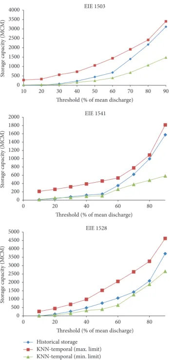
capacity lies between the range of minimum and maximum limits calculated from the generated data at all stations. This indicates the ability of the approach to effectively preserve the historical storage capacities. Actually, the range of minimum and maximum limits calculated from simulation is wide in all stations and the station EIE1528 shows the best results as the historical storage capacity line falls almost in the

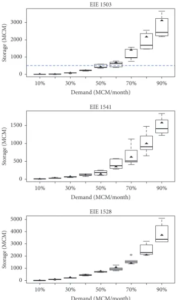
middle of the minimum and maximum limits plots. The sequent peak algorithm runs for different demand levels with the historical flow denoted as a triangle and each trace of simulated series (boxplots) shown in Figure 8. It can be observed that the approach provides a variable storage and the simulated results variability increases relevantly with the storage. Consider that the dash line in station EIE1503

(8)

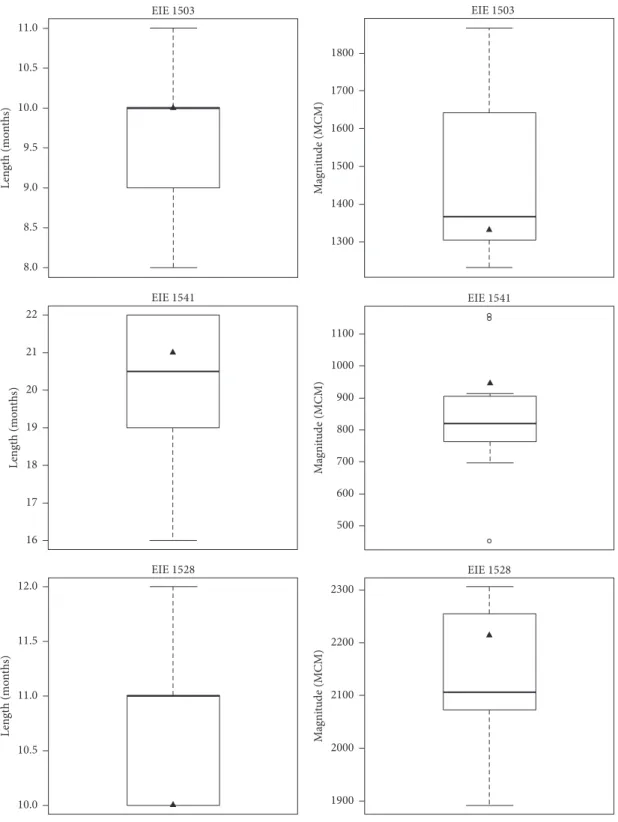
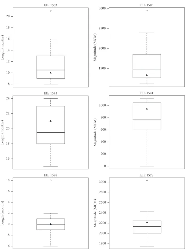
EIE1541 EIE1528 EIE 1503 10.0 10.5 11.0 11.5 12.0 Le n gth ( m o n th s) 16 17 18 19 20 21 22 Le n gth ( m o n th s) 8.0 8.5 9.0 9.5 10.0 10.5 11.0 Le n gth ( m o n th s) (a) EIE₁₅₄₁ EIE₁₅₂₈ EIE 1503 1900 2000 2100 2200 2300 M agni tude (M CM) 500 600 700 800 900 1000 1100 M agni tude (M CM) 1300 1400 1500 1600 1700 1800 M agni tude (M CM) (b)

Figure 6: Boxplots of length (a) and magnitudes (b) of maximum monthly droughts from the temporal approach. The triangle denotes the observed values.

(9)

EIE 1541

EIE 1528

Historical storage

20 30 40 50 60 70 80 90

10

Threshold (% of mean discharge) 0 500 1000 1500 2000 2500 3000 3500 4000 St o rag e ca paci ty (M CM) 0 200 400 600 800 1000 1200 1400 1600 1800 2000 St o rag e ca paci ty (M CM) 20 40 60 80 0

Threshold (% of mean discharge)

0 500 1000 1500 2000 2500 3000 3500 4000 4500 5000 St o rag e ca paci ty (M CM) 20 40 60 80 0

KNN-temporal (min. limit) KNN-temporal (max. limit)

Figure 7: Monthly historical storage capacity and their limits calculated from the temporal approach at all stations.

represents the storage capacity of 500 MCM. For the demand of 50% of the mean discharge, the observed flow sequences need 445 MCM of storage capacity, while the simulations represent the interquartile range of storage capacities between 346.6 and 590 MCM. This means that about 30% of the storage capacity of simulations is more than 500 MCM and that shows 70% reliability. This variation from the temporal approach simulations can offer a good estimate of system reliability.

4.2. Spatial Disaggregation Results. This section presents the monthly flow results obtained from the spatial disaggregation

approach over the study area. The advantage of spatial disag-gregation model is the ability to provide reliable streamflow data and realistic spatial structures at each time step and that can be easily adapted to different regions. The performance of the model was evaluated using monthly statistics. Observed and disaggregated values were tabulated in Table 2 for some months (September, October, November, January, and Febru-ary). It can be seen from Table 2 that the model preserved the mean and variance statistics in all stations and it can capture the skewness for all months very well, especially at low flow months (September and October) at all stations. The minimum and maximum simulated values show the ability of

(10)

T a b le 2: Som e m on th ly sp at ia l𝐾 NN st at ist ics fo r al lst at io ns . St at is ti c Se p tem b er O ct ob er N o ve m b er Ja n u ar y F eb ru ar y H ist o ric Dis ag gr ega te d H ist o ri c D is ag gr ega ted H ist o ric Dis ag gr ega te d H ist o ri c D is ag gr ega ted H ist o ric Dis ag gr ega te d St at io n E IE 15 28 M ea n 29 .1 9 32.6 1 4 2.4 6 4 1.1 62.7 62.7 94.86 95.2 4 12 3.7 12 4 .3 V ar ia n ce 10 4.6 5 10 2.8 19 0.8 1 19 0.4 808.8 76 2.8 25 57 .3 247 5.1 34 4 4 .5 31 92 .3 Sk ew 0.8 16 0.86 0.7 0 62 0.8 3 2.3 9 6 2.01 2.6 2 2.012 0.9 30 1 1.7 25 M in. 13.5 13.5 4 15.6 16.8 3 24.9 28.6 9 35.7 17 .2 84 54.4 14 .3 M ax. 53 .6 59 .1 82 .7 80.6 9 18 4.7 16 5.6 322 20 3 297 .1 198.9 St at io n E IE 15 41 M ea n 5.7 0 8 5.86 10.1 9. 86 16.08 16.08 30.2 4 30.5 6 37 .6 5 37 .7 8 V ar ia n ce 12.9 12.6 25 .1 23 .7 59 .6 55 .8 38 7. 6 37 3.6 43 8.1 41 7. 8 Sk ew 1.13 1.11 0.805 0.9 2 1.0 2 0.6 03 1.6 18 0.9 15 0.98 1.0 35 M in. 1.2 5 1.5 6 2.3 7 2.7 31 3.3 3 0.7 02 1 11.5 3 2.0 4 2 10.3 5.6 4 M ax. 17 .2 16.7 5 24.2 21.1 9 36.6 32 .6 2 95.8 5 73 .2 4 101 80.95 St at io n E IE 15 03 M ea n 27 .08 27 .05 33 .9 2 34.05 45.0 6 4 5.0 6 58.11 58.11 70.1 70 .1 7 V ar ia n ce 32 .6 31 .6 9 59 .18 6 0.5 2 31 7.1 30 2.4 721.4 69 2.2 126 6.3 12 32.1 Sk ew 0.6 8 0.7 3 0.5 1 0.5 6 2.87 1.9 9 2.8 15 2.4 28 1.7 41 1.13 M in. 17 .16 15.57 18.9 3 18.2 21.95 16.3 5 26.7 1 10.226 36.5 9 14.8 9 M ax. 4 0.8 9 39 .11 53 .9 55 .6 6 12 7.8 10 9.41 18 4.8 113.5 19 7. 5 16 5.4

(11)

EIE1528 EIE1541 0 1000 2000 3000 St o rag e (M CM) 30% 50% 70% 90% 10% Demand (MCM/month) 0 500 1000 1500 St o rag e (M CM) 30% 50% 70% 90% 10% Demand (MCM/month) 0 1000 2000 3000 4000 5000 St o rag e (M CM) 30% 50% 70% 90% 10% Demand (MCM/month)

Figure 8: Sequent peak results based on the demand of 10–90% of mean discharge from the temporal approach. The triangle denotes the observed values.

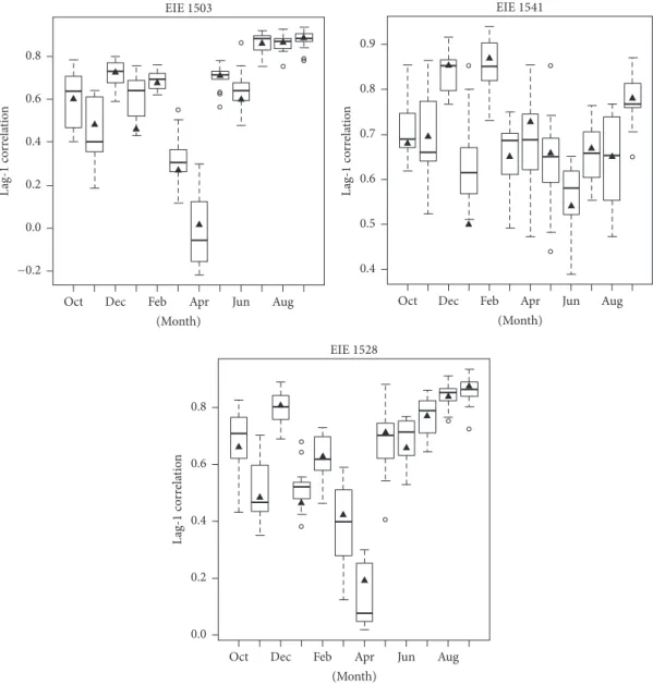
the approach to capture these two statistics for most months. For lag-1 correlation statistic, Figure 9 shows that the spatial approach preserves well the historical statistic, especially in low flow months through the convergence of the historical value with the median of simulated values. It can be seen that only the last month of the year and the first month of the next year (December-January) are not captured well in all stations. The performance of the model in reproducing the monthly streamflow is satisfactory, especially for the skew statistic.

To evaluate the performance of the approach in capturing the drought characteristics, the maximum drought length and magnitude were computed. The maximum monthly drought period lengths demonstrated a good preservation of the historical maximum drought length (Figure 10(a)). In addition, the maximum length drought has a varying length in the boxplots at all stations. This means that the approach generated more drought values than the historic

record. The maximum magnitudes of drought (Figure 10(b)) are captured within the interquartile rang at all stations, though they tend to be over- and underrepresented at EIE1503 and EIE1528 stations, respectively. The storage capacity results displayed in Figure 11 show that the his-torical storage capacity data lie virtually in the center of the maximum and the minimum plots. Also, the histor-ical storage capacity is very near to the limits through the range (10–50%) of the mean discharge. This indicates that the approach preserves the historical storage capacities efficiently.

For any selected storage capacity, we can find the demand level corresponding to it as shown in Figure 12. For example, the dashed line represents the storage capac-ity of 500 MCM at the site EIE1503. So, it can be seen that the spatial approach strongly overestimate storages for demand below the 40% of mean discharge and that about 90% of the needed storage is over than 500 MCM

(12)

EIE1541 EIE 1503 EIE1528 −0.2 0.0 0.2 0.4 0.6 0.8 La g-1 co rr ela tio n 0.4 0.5 0.6 0.7 0.8 0.9 La g-1 co rr ela tio n Jun Feb

Oct Dec Apr Aug

(Month)

Jun Feb

Oct Dec Apr Aug

(Month) 0.0 0.2 0.4 0.6 0.8 La g-1 co rr ela tio n Jun Feb

Oct Dec Apr Aug

(Month)

Figure 9: Simulated and observed lag-1 values from all stations. The triangle denotes the observed values.

for demand 50%. This variation from the spatial approach simulations can give a good reliable estimation of the system.

The comparison between the storage capacity charac-teristics of the observed and the generated data from the temporal and spatial approaches at all stations is shown in Figure 13. The results indicate that the storage capacities are reproduced very well when the threshold is taken as 60% of the mean discharge or less. The difference between the historical and simulation data is then increased progressively. In addition, it can be seen that best results are obtained when applying the spatial approach to all stations. This result supports the utilization of spatial approach since it gives a good improved storage capacity compared to temporal approach.

5. Conclusions

This study discusses the efficiency of the nonparametric disaggregation streamflow model to generate monthly flow series. The model was applied at three stations at

Kızılırmak River in Turkey. The model is based on𝐾-nearest

neighbor (𝐾NN) approach to resample the proportion vectors of monthly flow data from annual data. Historical annual streamflows were used to examine the performance of the model in generating monthly flow data. For comparison, the model was employed in both temporal and spatial approaches. The results show that the model can reproduce historical data in space and time domain, especially for the first two moments (mean and variance), and can also reproduce the continuity of the flows of the historical data at all stations. The spatial approach is showed to

(13)

EIE1528 EIE₁₅₄₁ EIE 1503 6 8 10 12 14 16 18 Le n gth ( m o n th s) 16 18 20 22 24 Le n gth ( m o n th s) 8 10 12 14 16 18 20 Le n gth ( m o n th s) (a) EIE1528 EIE₁₅₄₁ EIE 1503 1800 2000 2200 2400 2600 2800 3000 M agni tude (M CM) 0 200 400 600 800 1000 M agni tude (M CM) 1500 2000 2500 3000 M agni tude (M CM) (b)

Figure 10: Boxplots of length (a) and magnitudes (b) of maximum monthly droughts from the spatial approach. The triangle denotes the observed values.

(14)

EIE 1503 EIE 1541 EIE 1528 Historical storage 20 30 40 50 60 70 80 90 10

Threshold (% of mean discharge) 0 500 1000 1500 2000 2500 3000 3500 4000 4500 St o rag e ca paci ty (M CM) 0 200 400 600 800 1000 1200 1400 1600 1800 2000 St o rag e ca paci ty (M CM) 10 20 30 40 50 60 70 80 90 0

0 500 1000 1500 2000 2500 3000 3500 4000 4500 5000 St o rag e ca paci ty (M CM) 10 20 30 40 50 60 70 80 90 0

KNN-temporal (min. limit) KNN-temporal (max. limit)

Figure 11: Monthly historical storage capacity and its limits calcu-lated from the spatial approach at all stations.

be the best through overall results. The main advantage of spatial approach is the ability to obtain values at each time step and the flexibility to get values at several stations from one station, while the major drawback of both approaches was the inability to preserve the continuity between the last month of a year and the first month of the following year. Additionally, the monthly analysis of maximum drought length and magnitude offered a good preservation of the observed data characteristics. The results of drought analysis indicated that the spatial approach performs better when compared with temporal approach. In addition, the simulations generated a rich variety of dry

EIE1528 EIE1541 EIE 1503 0 1000 2000 3000 4000 St o rag e (M CM) 30% 50% 70% 90% 10% Demand (MCM/month) 30% 50% 70% 90% 10% Demand (MCM/month) 0 500 1000 1500 St o rag e (M CM) 30% 50% 70% 90% 10% Demand (MCM/month) 0 500 1000 1500 2000 2500 3000 3500 St o rag e (M CM)

Figure 12: Sequent peak results based on the demand of 10–90% of mean discharge from spatial approach. The triangle denotes the observed values.

sequences that will be of great benefit to manage water resources in the basin. The threshold used to determine drought statistics are based on the average of the historical flow. This threshold has been sensitized by the length of the historical data and can be adjusted as required for each basin. So, the various demands and storages founded from the sequent peak algorithm are considered a good way to identify drought analysis. However, the results of the storage capacity analysis obtained from the spatial and temporal approaches are found to preserve the historical data in Figures 7 and 11. In a conclusion, the nonparametric

disaggregation streamflow based on 𝐾NN approach

showed efficacy in producing monthly flow values, and the spatial approach is found to be a favorite choice for future hydrological applications at this region in Turkey.

(15)

EIE 1541 EIE 1528 Historical Spatial disaggregation Temporal disaggregation 0 500 1000 1500 2000 2500 3000 3500 St o ra ge ca paci ty (M CM) 20 30 40 50 60 70 80 90 10

0 200 400 600 800 1000 1200 1400 1600 1800 St o rag e ca paci ty (M CM) 10 20 30 40 50 60 70 80 90 0

0 500 1000 1500 2000 2500 3000 3500 4000 St o rag e ca paci ty (M CM) 10 20 30 40 50 60 70 80 90 0

Figure 13: Monthly storage capacity calculated using historical flow and data generated by spatial and temporal disaggregation approaches in all stations.

Competing Interests

The authors declare that they have no competing interests.

Acknowledgments

Shatha H. D. Al-Zakar and Omar M. A. Mahmood Agha thank the University of Mosul, Department of Dams and Water Resources Engineering, Mosul, Iraq, for giving them the opportunity to pursue their Ph.D. degree studies at the University of Gaziantep.

References

[1] D. Pumo, F. Viola, and L. V. Noto, “Generation of natural runoff monthly series at ungauged sites using a regional regressive model,” Water, vol. 8, no. 5, article no. 209, 2016.

[2] D. R. Valencia and J. C. Schakke, “Disaggregation processes in stochastic hydrology,” Water Resources Research, vol. 9, no. 3, pp. 580–585, 1973.

[3] J. D. Salas, J. W. Delleur, V. Yevjevich, and W. L. Lane, Applied

Modeling of Hydrologic Time Series, Water Resources

(16)

[4] J. M. Mejia and J. Rousselle, “Disaggregation models in hydrol-ogy revisited,” Water Resources Research, vol. 12, no. 2, pp. 185– 186, 1976.

[5] W. L. Lane, “Corrected parameter estimates for disaggregation schemes,” in Statistical Analysis of Rainfall and Runoff, V. P. Singh, Ed., Water Resources Publications, Littleton, Colo, USA, 1982.

[6] D. Koutsoyiannis and A. Manetas, “Simple disaggregation by accurate adjusting procedures,” Water Resources Research, vol. 32, no. 7, pp. 2105–2117, 1996.

[7] M. S. Mondal and S. A. Wasimi, “Disaggregation model for synthetic stream-flow generation,” Journal of Civil Engineering

(IEB), vol. 33, no. 1, pp. 43–54, 2005.

[8] D. Koutsoyiannis, “Coupling stochastic models of different timescales,” Water Resources Research, vol. 37, no. 2, pp. 379–391, 2001.

[9] D. G. Tarboton, A. Sharma, and U. Lall, “Disaggregation proce-dures for stochastic hydrology based on nonparametric density estimation,” Water Resources Research, vol. 34, no. 1, pp. 107–119, 1998.

[10] J. Prairie, B. Rajagopalan, U. Lall, and T. Fulp, “A stochas-tic nonparametric technique for space-time disaggregation of streamflows,” Water Resources Research, vol. 43, no. 3, 2007. [11] K. Nowak, J. Prairie, B. Rajagopalan, and U. Lall, “A

non-parametric stochastic approach for multisite disaggregation of annual to daily streamflow,” Water Resources Research, vol. 46, no. 8, Article ID W08529, 2010.

[12] J. M. Molina, Stepwise nonparametric disaggregation for daily

streamflow generation conditional on hydrologic and large-scale climatic signals [M.S. thesis], Colorado State University, 2010.

[13] Y. G. Dialynas, S. Kozanis, and D. Koutsoyiannis, “A computer system for the stochastic disaggregation of monthly into daily hydrological time series as part of a three-level multivariate scheme,” in Proceedings of the European Geosciences Union

General Assembly, vol. 13, Vienna, Austria, 2011.

[14] J. R. Prairie, B. Rajagopalan, T. J. Fulp, and E. A. Zagona, “Modi-fied K-NN model for stochastic streamflow simulation,” Journal

of Hydrologic Engineering, vol. 11, no. 4, pp. 371–378, 2006.

[15] A. T. Silva and M. M. Portela, “Disaggregation modelling of monthly streamflows using a new approach of the method of fragments,” Hydrological Sciences Journal, vol. 57, no. 5, pp. 942– 955, 2012.

[16] N. Rebora, F. Silvestro, R. Rudari, C. Herold, and L. Ferraris, “Downscaling stream flow time series from monthly to daily scales using an auto-regressive stochastic algorithm: Stream-FARM,” Journal of Hydrology, vol. 537, pp. 297–310, 2016. [17] U. Lall and A. Sharma, “A nearest neighbor bootstrap for

resampling hydrologic time series,” Water Resources Research, vol. 32, no. 3, pp. 679–693, 1996.

[18] U. Lall, “Recent advances in nonparametric function estima-tion: hydrologic applications,” Reviews of Geophysics, vol. 33, no. S2, pp. 1093–1102, 1995.

[19] N. S¸arlak, “Annual streamflow modelling with asymmetric distribution function,” Hydrological Processes, vol. 22, no. 17, pp. 3403–3409, 2008.

[20] D. P. Loucks, J. R. Stedinger, and D. A. Haith, Water Resources

Systems Planning and Analysis, Prentice-Hall, 1981.

[21] T. A. Awchi and D. K. Srivastava, “Analysis of drought and stor-age for Mula project using ANN and stochastic generation models,” Hydrology Research, vol. 40, no. 1, pp. 79–91, 2009.

(17)