Estimating bankruptcy probability using fuzzy logic: an application to a panel of us and Turkish industries

T. C.

KADİR HAS UNIVERSITY

INSTITUTE OF SOCIAL SCIENCES

FINANCE AND BANKING

ESTIMATING BANKRUPTCY PROBABILITY

USING FUZZY LOGIC: AN APPLICATION TO A

PANEL OF US AND TURKISH INDUSTRIES

PH.D DISSERTATION

Çigdem ÖZARI

Thesis Advisor

Prof.Dr. VEYSEL ULUSOY

T. C.

KADİR HAS UNİVERSİTESİ

SOSYAL BİLİMLERİ ENSTİTÜSÜ

BANKACILIK VE FINANS

MİKRO PANEL VERİ ANALİZİ VE BULANIK MANTIK

METODOLOJİSİ İLE FİRMALARIN PİYASADAN

ÇEKİLME OLASILIKLARININ TAHMİNİ: TÜRK VE

AMERİKAN FİRMALARI ÜZERİNE BİR UYGULAMA

DOKTORA TEZİ

Çigdem ÖZARI

Thesis Advisor

Prof.Dr. VEYSEL ULUSOY

LIST OF ABBREVATIONS ... X ACKNOWLEDGMENT ... XI ABSTRACT... XII ÖZET ... XIII

INTRODUCTION ... 1

CHAPTER 1 FACTOR ANALYSIS ... 4

CHAPTER 2 PROBABILITY OF DEFAULT & METHODS FOR ESTIMATING DEFAULT PROBABILITIES ... 8

2.1. PROBABILITY OF DEFAULT ... 8

2.2. METHODS FOR ESTIMATING DEFAULT PROBABILITIES ... 9

2.3. LITERATURE ... 11

2.4 MERTON MODEL AND ITS EXTENSIONS ... 13

2.4.1 Merton Model ... 13

2.4.1.1 Assumptions of Merton Model ... 16

2.4.2.1Simplification of Distance to Default ... 27

2.5 DEFAULT & SURVIVAL PROBABILITIES ... 29

2.5.1 Bivariate Normal Distribution ... 29

2.6 AN APPLICATION OF PUBLIC COMPANIES IN TURKEY ... 33

CHAPTER 3 CLUSTER ANALYSIS & FUZZY LOGIC ... 43

3.1 CLUSTER ANALYSIS ... 43

3.1.1 A TYPOLOGY OF CLUSTERING ... 47

3.1.1.1 Hierarchic versus Nonhierarchical (Partional) Methods ... 48

3.1.1.2 Agglomerative versus Divisive Methods ... 50

3.1.1.3 Nonoverlapping versus Overlapping Methods ... 50

3.1.2 CLUSTERS ... 51

3.1.2.1 Single Link Method ... 52

3.1.2.2 Complete Link Method ... 52

3.1.2.3 Group Average Link... 53

3.1.3 FUZZY CLUSTERING ... 54

3.1.4 LIMITATIONS OF CLUSTERING (ADVANTAGES & DISADVANTAGES OF CLUSTER ANALYSIS) ... 54

3.2 FUZZY LOGIC ... 55

3.2.1 FUZZY SETS & MEMBERSHIP FUNCTIONS ... 60

3.2.1.1 Fuzzy Sets ... 60

3.2.1.1.1 Definition of a Fuzzy Set ... 61

3.2.1.2 Membership Functions and Fuzzy Numbers ... 63

3.2.1.2.1 Triangular Membership Functions ... 63

3.2.1.2.2 A Trapezoidal Membership Functions ... 64

3.2.3 OPERATIONS ON FUZZY SETS ... 66

3.2.4 FUZZY INFERENCE SYSTEM ... 70

3.2.4.1 Fuzzification ... 73

3.2.4.2 Rule Generation ... 74

3.2.4.3 Defuzzification ... 77

CHAPTER 4 THE MODEL AND DATA ... 81

4.1 DATA ... 82

4.2 FACTOR ANALYSIS & CLUSTERING PART ... 83

4.3 THE MODEL (PROBABILITY OF DEFAULT) ... 102

4.4 Fuzzy Model for Bankruptcy Probability ... 108

CHAPTER 5 MACRO ECONOMIC FACTORS & PROBABILITY OF DEFAULT ... 115

CONCLUSION ... 119

APPENDICES ... 122

I. BARRIER OPTIONS ... 122

II. VARIANCE FORMULATION ... 123

III. INTEREST RATES FOR ISE100 APPLICATION ... 123

IV. MACRO FOR GOAL SEEK FUNCTION ... 124

V. RESULTS OF ISE100 APPLICATION ... 125

VI. DEFINITIONS OF RATIOS ... 131

VII. CLUSTERING RESULTS ... 135

VIII MPD RESULTS OF USA INDUSTRIES ... 141

IX DISTANCE TO DEFAULT ... 143

X. MEMBERSHIP FUNCTIONS OF INPUT VARIABLES ... 143

LIST OF GRAPHS

GRAPH 2.1MPD OF SELECTED IMKBCOMPANIES ... 35

GRAPH 2.2MPD OF SELECTED COMPANIES FROM ISE100 ... 36

GRAPH 2.3DD OF SELECTED COMPANIES FROM ISE100 ... 38

GRAPH 2.4EDF OF SELECTED COMPANIES FROM ISE100 ... 40

GRAPH 2.5MPD-DD-EDF OF COMPANIES ... 41

GRAPH 2.6CORRELATIONS BETWEEN DEFAULT PARAMETERS ... 42

GRAPH 4.1MPD OF FOREIGN USACOMPANIES ... 108

GRAPH 4.2MEMBERSHIP FUNCTIONS OF INPUT VARIABLE;NSH ... 111

GRAPH 4.3SURFACE THAT SHOWS RELATIONSHIP BETWEEN SP,MPD AND OUTPUT ... 114

GRAPH 5.1.AFBI&CPI AND MPD&IP ... 118

GRAPH 5.1.BMPD&SPI AND MPD&UR ... 118

GRAPH VII.1CLUSTERS PERCENTAGE AT 2005 ... 135

GRAPH VII.2WITHIN CLUSTER PERCENTAGE OF INDUSTRY (2005) ... 136

GRAPH VII.3CLUSTERS PERCENTAGE AT 2006 ... 137

GRAPH VII.4WITHIN CLUSTER PERCENTAGE (2006) ... 137

GRAPH VII.5CLUSTER PERCENTAGE AT 2007 ... 138

GRAPH VII.6WITHIN CLUSTER PERCENTAGE (2007) ... 139

GRAPH VII.7CLUSTERS PERCENTAGE AT 2008 ... 140

GRAPH VII.8WITHIN CLUSTER PERCENTAGE (2008) ... 140

GRAPH X.1MEMBERSHIP FUNCTION OF THE INPUT VARIABLE:SP ... 144

GRAPH X.2MEMBERSHIP FUNCTION OF THE INPUT VARIABLE:NSH ... 144

GRAPH X.3MEMBERSHIP FUNCTION OF THE INPUT VARIABLE:EBIT ... 145

GRAPH X.4MEMBERSHIP FUNCTION OF INPUT VARIABLE:EV/TS ... 145

GRAPH X.5MEMBERSHIP FUNCTION OF THE INPUT VARIABLE:MPD ... 146

GRAPH X.6MEMBERSHIP FUNCTION OF THE OUTPUT VARIABLE ... 146

GRAPH X.7FUZZY RESULT OF OUTPUT VARIABLE ... 147

GRAPH X.8SURFACE THAT SHOWS RELATIONSHIP BETWEEN EBIT,MPD AND OUTPUT ... 149

GRAPH X.9SURFACE THAT SHOWS RELATIONSHIP BETWEEN EV/TS,MPD AND

OUTPUT ... 149

GRAPH X.10SURFACE THAT SHOWS RELATIONSHIP BETWEEN NSH,MPD AND

LIST OF TABLES

TABLE 2.1DEFAULT AND NO DEFAULT CASES ... 15

TABLE 2.2VALUE OF PORTFOLIO AT TIME T ... 16

TABLE 2.3.ARESULTS OF ITERATIONS ... 26

TABLE 2.3.BJACOBIAN AND INVERSE JACOBIAN MATRIX ... 26

TABLE 2.4MPD OF COMPANIES SELECTED FROM ISE100(2004-2008)... 34

TABLE 2.5DD OF SELECTED ISE100COMPANIES (2004-2008) ... 37

TABLE 2.6EDF OF SELECTED ISE100COMPANIES (2004-2008) ... 39

TABLE 2.7CORRELATIONS BETWEEN DEFAULT PARAMETERS ... 41

TABLE 3.1FORMULAS OF DISTANCE FUNCTIONS ... 45

TABLE 3.2EXAMPLE FOR RULE GENERATION ... 76

TABLE 4.1FINANCIAL RATIOS ... 81

TABLE 4.2FINANCIAL RATIOS ... 82

TABLE 4.3.AFACTOR ANALYSIS ... 83

TABLE 4.3.BFACTOR ANALYSIS ... 84

TABLE 4.3.CFACTOR ANALYSIS ... 85

TABLE 4.4NUMBER OF COMPANIES ... 86

TABLE 4.5CLUSTER ANALYSIS OF FOREIGN USACOMPANIES AT 2005 ... 90

TABLE 4.6CLUSTER ANALYSIS OF FOREIGN USACOMPANIES AT 2006 ... 91

TABLE 4.7CLUSTER ANALYSIS OF FOREIGN USACOMPANIES AT 2007 ... 93

TABLE 4.8CLUSTER ANALYSIS OF FOREIGN USACOMPANIES AT 2008 ... 94

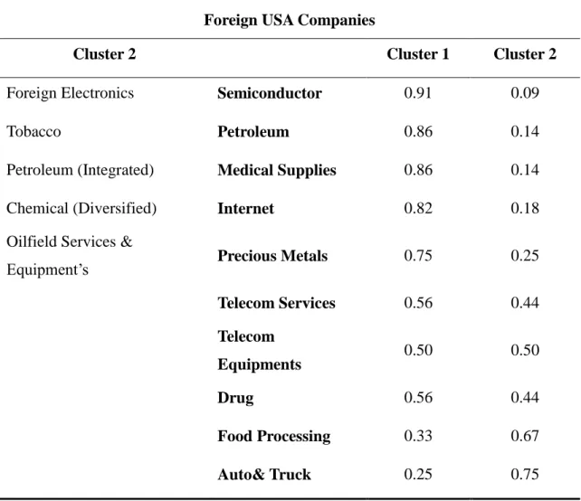
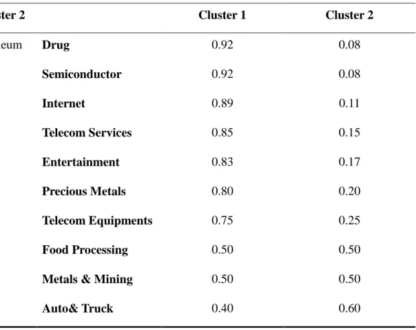
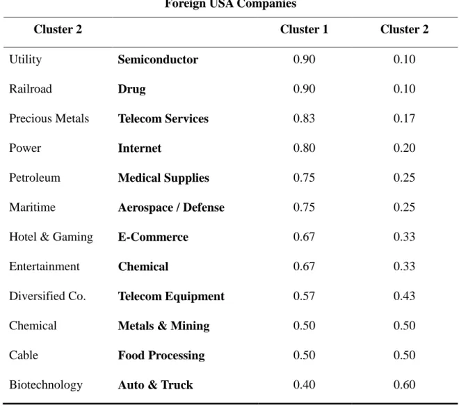
TABLE 4.9INDUSTRIES BETWEEN CLUSTERS ... 95

TABLE 4.10DESCRIPTIVE STATISTICS OF ALL INDUSTRIES ... 96

TABLE 4.11DESCRIPTIVE STATISTICS OF THE INDUSTRY:SEMICONDUCTOR (BETWEEN CLUSTERS) ... 97

TABLE 4.12DESCRIPTIVE STATISTICS OF THE INDUSTRY:INTERNET (BETWEEN CLUSTERS) ... 97

TABLE 4.13DESCRIPTIVE STATISTICS OF THE INDUSTRY:DRUG (BETWEEN CLUSTERS) ... 98 TABLE 4.14DESCRIPTIVE STATISTICS OF THE INDUSTRY:AUTO &TRUCK (BETWEEN

CLUSTERS) ... 99

TABLE 4.15CORRELATION MATRIX ... 100

TABLE 4.16MPD OF THE INDUSTRIES WHICH ARE BETWEEN CLUSTERS IN 2005 ... 104

TABLE 4.17MPD OF THE INDUSTRIES WHICH ARE BETWEEN CLUSTERS IN 2006 ... 104

TABLE 4.18MPD OF THE INDUSTRIES WHICH ARE BETWEEN CLUSTERS IN 2007 ... 105

TABLE 4.19MPD OF THE INDUSTRIES WHICH ARE BETWEEN CLUSTERS IN 2008 ... 106

TABLE 4.20UPPER AND LOWER BOUNDS (2005) ... 107

TABLE 4.21DEFAULT CORRELATION BOUNDARIES OF INDUSTRIES ... 108

TABLE 4.22.ARANGE OF THE VARIABLES ... 109

TABLE 4.22.BRANGE OF THE VARIABLES ... 109

TABLE 4.22.BRANGE OF THE VARIABLES ... 110

TABLE 4.22.CRANGE OF THE VARIABLES AND MODEL PROPERTIES ... 110

TABLE 5.1ESTIMATES OF FIXED EFFECTS FOR INDUSTRY ... 117

TABLE III.1RISK FREE INTEREST RATES BETWEEN 2004-2008RISK-FREE INTEREST RATES... 124

TABLE V.1VOLATILITY OF FIRM’S ASSET RETURNS ... 126

TABLE V.2MARKET VALUE OF FIRM’S ASSET RETURN ... 127

TABLE V.4CORRELATION BETWEEN MERTON MODEL PARAMETERS AT 2004 ... 128

TABLE V.6CORRELATION BETWEEN MERTON MODEL PARAMETERS AT 2006 ... 129

TABLE V.7CORRELATION BETWEEN MERTON MODEL PARAMETERS AT 2007 ... 130

TABLE V.82008CORRELATION BETWEEN MERTON MODEL PARAMETERS AT 2008 . 130 TABLE VII.1CLUSTER DESCRIPTIVE STATISTICS (2005) ... 136

TABLE VII.2CLUSTER DESCRIPTIVE STATISTICS (2005) ... 137

TABLE VII.3CLUSTER DESCRIPTIVE STATISTICS (2006) ... 138

TABLE VII.4CLUSTER DESCRIPTIVE STATISTICS (2006) ... 138

TABLE VII.5CLUSTER DESCRIPTIVE STATISTICS (2007) ... 139

TABLE VII.6CLUSTER DESCRIPTIVE STATISTICS (2007) ... 139

TABLE VII.7CLUSTER DESCRIPTIVE STATISTICS (2008) ... 140

TABLE VII.8CLUSTER DESCRIPTIVE STATISTICS (2008) ... 141

TABLE VIII.1MERTON DEFAULT PROBABILITIES OF INDUSTRIES ... 142

LIST OF FIGURES

FIGURE 3.1EXAMPLES OF CLUSTER TYPES ... 44

FIGURE 3.2TYPOLOGY OF CLUSTERING ... 47

FIGURE 3.3DENDOGRAM ... 48

FIGURE 3.4CLUSTER A&CLUSTER B ... 51

FIGURE 3.5SINGLE LINK METHOD ... 52

FIGURE 3.6COMPLETE LINK METHOD ... 53

FIGURE 3.7GROUP AVERAGE LINK METHOD ... 53

FIGURE 3.8ATRIANGULAR FUZZY NUMBER ... 64

FIGURE 3.9ATRAPEZOIDAL FUZZY NUMBER ... 65

FIGURE 3.10COMPLEMENT OF A FUZZY SET ... 66

FIGURE 3.11UNION OF FUZZY SETS ... 67

FIGURE 3.12INTERSECTION OF FUZZY SETS ... 67

FIGURE 3.13FUZZY INFERENCE SYSTEMS ... 72

FIGURE 3.14INFERENCE ENGINE ... 72

FIGURE 3.15DEFUZZIFICATION METHODS ... 78

FIGURE 3.16SUGENO MODEL ... 79

FIGURE 4.1MAXIMUM CORRELATION COEFFICIENT -I ... 100

FIGURE 4.2MAXIMUM CORRELATION COEFFICIENT –II ... 101

FIGURE 4.3FUZZY SYSTEM OF OUR MODEL... 111

FIGURE 4.4SUMMARY OF “FUZZY IF THEN”RULES ... 113

LIST OF ABBREVATIONS

MPD Merton Default Probability

DD Distance to Default

EDF Expected Default Frequency

SP Stock Price

BVL Beta Value Line

TD Total Debt

CF Cash as Firm Value

NSh Number of Shares Outstanding

TV Trading Volume

TS Trailing Sales

EG Expected Growth in EPS

PTOM Pre-tax Operating Margin

St. Dev. Standard Deviation

IPI Industrial Production Index

CPI Consumer Price Index

IR Interest Rate Spread

SPI Share Price Index

UR Unemployment Rate

FOI Financial Openness Index

GDP Gross Domestic Product

PS Price to Sales Ratio

PBV Price Book Value Ratio

FCFF Free Cash Flow for the Firm

ACKNOWLEDGMENT

I am heartily thankful to my supervisor, Prof. Dr. Veysel Ulusoy, whose stimulating suggestions, encouragement, guidance and support from the initial to the final level enabled me to develop an understanding of the subject.

Also I would to thank Kadir Has University colleagues for helping me to broaden my view and knowledge. Especially, I would like to give my special thanks to Doç. Dr. Hasan Eken for giving me the opportunity to work with Prof. Dr. Veysel Ulusoy.

Lastly, I offer my regards and blessings to all of those who supported me in any respect during the completion of this thesis.

ABSTRACT

The main purpose of this study is to show how a Merton Model approach can be used to develop a new measure of company failures’ probability independent from their sectors. In this study, a new index, Fuzzy-bankruptcy index, is created which explains the default probability of any firm X, independent from the sector it belongs. In the construction process in order to reduce the relativity of financial ratios due to the fact that their interpretation change with time and according to different sectors, fuzzy logic is used. For the fuzzy process, we used five input variables, four of them are chosen from both factor analysis and clustering and the last input variable calculated from Merton Model. Looking back to the default history of firms, one can find different reasons such as managerial arrogance, fraud and managerial mistakes which are responsible for the very sad endings of well-known companies like Enron, K-Mart and even the country Argentina. Thus, we hope with the help of our Fuzzy-bankruptcy index one could be able to get a better insight into the financial situation a company is in, and it could also prevent credit loan companies from investing in the wrong firm and possibly from losing the entire investment.

This study is organized as seven chapters. Chapter one explains the factor analysis. Chapter two gives the definition of probability of default and outlines the methods for estimating default probability. It reviews the literature on estimating the default probabilities, the Merton Model and its extensions. Chapter three explains the cluster analysis and fuzzy logic. It reviews the literature on clustering and methods of clustering, especially explains the method of how to cluster variables in detail. Second part of chapter three explains fuzzy logic and its applications. It reviews the literature on applications of fuzzy logic and how and why we use fuzzy logic in our model. Chapter four gives the information of our study and describes the model we studied. Chapter five investigates the relationship between macro-economic factors and probability of default and Chapter six concludes. Chapter seven is appendix of our study.

ÖZET

Merton Model opsiyon fiyatlama yöntemini kullanarak finansal şirketlerin batma olasılıklarının hesaplanmasında kullanılan bir modeldir. Biz bu çalışmada, Merton Model kullanarak şirketlerin batma olasılıklarını hesapladık. Öncelikle, IMKB100 içinde yer alan finansal şirketler için Merton Model kullanarak batma olasılıklarını hesapladık, değerlerin sıfır ve bire çok yakın olduğunu ya da seneden seneye olan geçişlerde değişkenliğin çok yoğun olduğunu gözlemledik. Bu sonuçlarla çalışmamızdaki ana amacımızı, Merton Modeli de kullanarak, sektörden bağımsız, yani tüm şirketler için yorumlayabileceğimiz ve karşılaştırabileceğimiz bir endeks oluşturmak olarak değiştirdik. Literatürde, şirketlerin finansal durumlarını yorumlayabilmek için çok sayıda finansal rasyolar olduğunu ve bu finansal rasyoların yorumlarının firmaların ait olduğu sektörlerle de ilişkilendiği bilinmektedir. Bu ilişki yüzünden, oluşturmak istediğimiz endeksi bulanık mantık kullanarak oluşturmamız gerektiğine karar verdik. Literatürde çok sayıda yeterli ve anlamlı finansal rasyolarla karşılaştığımızdan, şirketlerin batma olasılıklarını yorumlayabilecek için her bir finansal rasyoya tek tek bakmak yerine; çok sayıda olan finansal rasyolara faktör analizi uygulayarak, aynı açıklamayı yapacak daha az sayıda finansal rasyolar belirledik. Ulaştığımız sayı bulanık mantık uygulamamızı kişiselleştireceğinden, faktör analizi ile elimine ettiğimiz finansal rasyoları kümeleme yöntemi kullanarak bir kez daha elimine ettik. Böylelikle, bulanık mantık kullanarak oluşturacağımız değişkenimizin girdi değişkenlerini belirlemiş olduk. Bu değişkenleri ve arasındaki ilişkiyi inceleyerek, değişkenler arasında kuralları belirleyerek modelimiz oluşturduk. Böylelikle Merton modeli de dâhil ederek, bulanık mantık kullanarak şirketlerin batma olasılıklarını daha hassas ve sektörden bağımsız olarak hesapladık. Son olarak bulduğumuz endeksi makroekonomik göstergelerle açıkladık.

INTRODUCTION

The main purpose of this study is to show how a Merton Model approach can be used to develop a new measure of company failures’ probability independent from their sectors. The original Merton model is based on some simplifying assumptions about the structure of the typical firm’s finances. The event of default is determined by the market value of the firm’s assets in conjunction with the liability structure of the firm.1

Merton approach is the most popular approach for estimating default probability by using market information. The model assumes that a firm has equity and certain amount of zero coupon debt that will become due at a future time. Much of the literature follows Merton (1974) by explicitly linking the risk of a firm’s bankruptcy to the variability in the firm’s asset value and by viewing the market value of firm’s equity as the standard call option2 on the market value of firm’s asset with strike price equal to the promised payment of corporate debts.3 Merton proposes that the position of the shareholders can be considered as similar to purchasing a call option on the assets of the company, and the price at which they will exercise this option to purchase is equal to the book value of company's debt due for payment in the defined time horizon. In this way, Merton was the first to demonstrate that a firm's option of defaulting can be modeled in accordance with the assumptions of Black and Scholes (1973).

In this study, a new index, Fuzzy-bankruptcy index, is created which explains the default probability of any firm X, independent from the sector it belongs. In the construction process in order to reduce the relativity of financial ratios due to the fact that their interpretation change with time and according to different sectors, fuzzy logic is used. For the fuzzy process, minimum number of input variables is used to construct

1 _{A Merton Model Approach to Assessing the Default Risk of UK Companies, Merxe Tudela and Garry}

Young; Bank of England; 2003.

2 _{Options are known from the financial world where they represent the right to buy or sell a financial}

value, mostly a stock, for a predetermined price, without having the obligation to do so. For more detail See: Carlsson, C.,Fuller,R.; Fuzzy Sets and Systems and J. Hull, Options, Futures and Derivatives

3 _{The Predictive Performance of a Barrier Option Credit Risk Model in an Emerging Market, David}

the output variable which denotes our bankruptcy probability. There are many different reasons why companies have defaulted over the time. Hot items in these are managerial arrogance, fraud and managerial mistakes. Well-known examples are companies like Enron, K-Mart and even the country Argentina. These causes are related with many other companies that defaulted over time. Thus, with the help of our Fuzzy-bankruptcy index one could be able to get a better insight into the financial situation a company is in, and it could also prevent credit loan companies from investing in the wrong firm and possibly from losing the entire investment.

This study is organized as five chapters. Chapter one starts explaining factor analysis, which is a data reduction method to resume a number of original variables into a smaller set of composite dimensions, or factors. This method is commonly used when developing a questionnaire to see the relationship between the items in the questionnaire and underlying dimensions. It is also used to reduce larger data set of variables to a smaller set of variables that explain important dimensions of variability.

Chapter two gives the definition of probability of default and outlines the methods for estimating default probability. It reviews the literature on estimating the default probabilities, the Merton Model and its extensions. In this chapter, Merton default probabilities of ISE100 financial companies from year 2004 to 2008 are calculated. Distance to Default (DD) and Expected Default Frequency (EDF) are also calculated as functions of Merton default probabilities.

Chapter three explains the cluster analysis and fuzzy logic. In the first part, the literature on clustering and methods of clustering are reviewed by showing special attention how to cluster variables in detail. Cluster analysis groups individuals or objects into clusters so that objects in the same cluster are homogeneous and there is heterogeneity across clusters. Homogeneous means data belongs the same clusters should be as similar as possible and heterogeneity means data belongs the different clusters should be as different as possible. In other words, we can group or cluster the observed data that the similarity of cases within each cluster is maximum and the dissimilarity of cases between clusters is maximum. Second part of chapter three explains fuzzy logic and its

applications. It reviews the literature on applications of fuzzy logic. Fuzzy logic is used due to the fact that fuzzy set theory is developed for solving problems in which descriptions of observations are imprecise, vague and uncertain. The term “fuzzy” refers to the situation in which there are no well- defined boundaries of the sets of activities or observations to which the descriptions apply. For example, one can easily assign a firm with Merton default probability is 0.6 to the “class of default firms, because the term default probability does not constitute a well-defined boundary. Chapter four gives the information of the study and describes the model we studied. Chapter five investigates the relationship between macro-economic factors and probability of default.

CHAPTER 1 FACTOR ANALYSIS

Factor Analysis is a branch of statistical science, however because of its extensions on psychology, the technique itself is often mistakenly considered as psychological theory. The origin of the factor analysis is generally ascribed to Charles Spearman4. Since his monumental work in developing psychology theory involving a single factor analysis.

Application of factor analysis in fields other than psychology has become very popular since 1950. These fields include such varied disciplines as medical, political science, economics, sociology, taxonomy. Also, there are many individual studies that are difficult to assign to a particular discipline. In economics, evaluating the performance of the systems5, investment decisions6, structure of security price changes were the subjects which are examples of factor analysis applications.

When we try to specify the economic relationships by mathematical formulation we encounter problems such as which variables should be included in the equation, what form they should be assume; linear, nonlinear, logarithmic; and whether a single equation may be analyzed independently or a complete model of simultaneous equations should be considered all at once. If the explained variable in one relationship became the explanatory variable in other equation the single relationship can not be analyzed independently. In specifying relationships, it is necessary to know first what variables should be included in the relationship as explanatory variables. One method which will tell us the significance of each explanatory variable in explaining the variation of the explained variable is factor analysis. The basic idea behind the factor analysis is to represent a set of variables by a smaller number of variables. In this case, they are called factors. The variables used in factor analysis should be linearly related to each other. In other words, the variables must be at least moderately correlated to each

4

English psychologist known for work in statistics as a pioneer of factor analysis and for Spearman’s rank correlation coefficient.

5 _{Burch, 1972.} 6 _{Farrar 1962.}

other; otherwise the number of factors will be almost the same as the number of original variables. This means that factor analysis is pointless.

Factor analysis could be used for any of the following purposes:

 To reduce a large number of variables to a smaller number of factors for modeling purposes

 To select a subset of variables from a larger set based on which original variables have the highest correlations with the principal component factors.

 To identify clusters of cases

 To create a set of factors to be treated as uncorrelated variables as one approach to handling multicollinearity in such procedures as multiple regression

 To establish that multiple tests measure the same factor, thereby giving justification for administering fewer tests. Factor analysis originated a century ago with Charles Spearman's attempts to show that a wide variety of mental tests could be explained by a single underlying intelligence factor (a notion now rejected, by the way).

In the following, we state the basic procedure of finding the factors by the principal axis method. First, we list all the variables that we think are in some way related. Suppose we have N such variables. We then collect sample data on these variables and compute a symmetric matrix M in such a way that on the diagonal of the matrix, we enter the square of the multiple correlation coefficient7 of one of the N variables in relation to the other variables. And off the diagonal of the matrix we enter the simple correlation

7 _{To measure the linear correlation between}

2

X ,X₃ and Y we use the correlation of multiple correlation;R_1.23. The square of R_1.23 is called the coefficient of determination. It is the ratio of explained variables and total variation of Y. Using simple correlation coefficients,

2 23 23 13 12 2 13 2 12 2 23 . 1 r 1 r r 2r r + r = R  

coefficients between each pair of the N variables. The matrix, which we called M, will be like the following:

) 1 + (N ) 1 + (N 2 ) 1 (N .123... N 2N 1N 1N 2 N 2.134... 12 12 2 N 1.234... R ... r r ... ... ... ... ... ... ... r ... ... ... ... ... ... R r ... ... r R M                   

Then, we perform row and column operations on matrix M to transform it into a diagonal matrix.

D = MB BT

, where B is orthogonal matrix8 and D is diagonal matrix, and BD

= MB

BBT . Since B is orthogonal matrix the transpose of B is the same as inverse of B, which meansBBT =I. Thus,MB=BD, where

                                         N 2 1 NN N1 2N 22 21 1N 12 11 λ .. ... 0 0 ... ... ... ... ... ... 0 ... 0 λ 0 0 .. 0 0 λ m ... ... ... m ... ... m ... ... m m m ... ... m m BD

Matrix D is diagonal matrix, on the diagonal are the characteristics roots λ and off the _i diagonal are all zeros. B matrix is called the matrix of characteristic vectors. Choose only positiveλ and arrange them in descending order. Multiplying λ by its i respective columnmji(j=1,2,...,N), we get vectors of coefficients. These coefficients

represent the contributions of each variable to each other.

Figure 1.1 Matrix Representation of Factor Analysis

Factor 1 Factor 2 … Factor K

Variable 1 Coefficient Coefficient Coefficient

Variable 2 … … … …

…. … … … …

… … … … …

Variable N … … … …

The coefficients in each vector whose values are very close may be grouped together and factors as defined by the grouped variables.

Now, we can summarize the steps in conducting a factor analysis. There are four basic factor analysis steps:

 data collection and generation of the correlation matrix

 extraction of initial factor solution

 rotation and interpretation

CHAPTER 2 PROBABILITY OF DEFAULT & METHODS

FOR ESTIMATING DEFAULT PROBABILITIES

There are several measures of country risk, one of the simplest and most easily accessible is the rating assigned to a country’s debt by ratings agency. These rating agencies measures the default risk rather than the equity risk. In addition, default risk is also affected by many of the factors that affect the equity risk. Note that the most obvious determinant of a company’s risk exposure to country risk is how much of the revenues it derives from the country.

2.1. PROBABILITY OF DEFAULT

A technical default is a delay in timely payment of an obligation, or a non-payment all together. If an obligor misses a payment, by even one day, it is said to be in technical default. This delay may be for operational reasons (and so not really a great worry) or it may reflect a short-term cash flow crisis, such as the Argentina debt9 default for three months. But if the obligor states it intends to pay the obligation as soon as it can, and specifies a time-span that is within (say) one to three months, then while it is in technical default it is not in actual default. If an obligor is in actual default, it is in default and declared as being in default. This does not mean a mere delay of payment. If an obligor does not pay, and does not declare an intention to pay an obligation, it may then be classified by the ratings agencies as being in ‘default’ and rated ‘D’.

Shortly, the default probability is the probability that the value of the assets of the firm will be less than the book value of its liabilities at the maturity. (Default probability is similar to expected default frequency used by Moody’s KMV10

) The probability of default is a function of two factors: 11

1. Ratio of debt (and other fixed costs) to cash flows: Default is the result of a firm

being unable to service its fixed claims. The larger is the size of cash flows on debt obligations and other fixed claims relative to the size of operating cash flows, the higher is the probability of default.

2. Volatility of Cash Flows: Default is triggered when the firm’s cash flow is too low to

pay its fixed claims. The more volatile the firm’s (operating) cash flow, the more likely it is that the firm will face default.

2.2. METHODS FOR ESTIMATING DEFAULT PROBABILITIES

Prior empirical models of corporate default probabilities, reviewed by Jones (1987) and Hillegeist, Keating, Cram and Lundstedt (2004), have relied on many types of covariates, both fixed and time varying. Academics in the fields of accounting and finance have actively studied bankruptcy prediction since the work of Beaver (1966, 1968) and Altman (1968). Altman’s z-score is a measure of leverage, defined as the market value of equity divided by the book value of total debt. And a second generation of empirical work is based on qualitative response models, such as logit and probit. Among these, Ohlson (1980) used an o-score method; effectively summarize publicly-available information about the probability of bankruptcy.

10

KMV is a trademark of KMV Corporation. Stephen Kealhofer, John Mc Quown and Oldrich Vasicek founded KMV Corporation in 1989. On February 11, 2002, Moody’s announced that it was acquiring KMV for more than $200 million in cash.

Credit risk models are gaining popularity in the light of the Basel II12 accord. The pioneers of estimation of default probabilities are rating agencies like Moody’s, Fitch and S&P. They started to publish not only the ratings of companies but also their estimated default probabilities. These estimations are produced from historical data. 13

2.2.1. Estimating Default Probabilities from Historical Data

In this method, rating agencies produce data for showing that default experience over pre-determined time period of bonds that had a particular rating at the beginning of the period. So, probability of a bond defaulting during a particular year can be calculated from the historical defaulting experience data which was prepared from the rating agencies.

To estimate the default probability from historical data, Stefan Huschens, Konstantin Vogl, and Robert Wania, first consider the homogeneous group. To simplify the model, first they assume all obligors have the same default probability. (i.e., pick all obligors with the same rating from a portfolio). In their study, they characterized obligors by a Bernoulli distribution14 and each obligor is independent form each other. For estimation of default probabilities one has to take into account that dependence affects the estimation. If one can relax the independence condition the next step is to consider the case of equicorrelation.15 They found closely connection between the default probability and the default correlation. Also, the estimation procedure has to take into account this relation. In their article, they present estimation methods for both, the general case of a Bernoulli mixture model and the special case of the single-factor model which is used in the Internal Ratings- Based Approach of Basel II.

12 _{Basel II is the second of the Basel accords.} 13

For further readingon estimation methods of rating agencies see Kavvathas (2000) and Carty (1997).

14 _{Take the value 1 if the obligor defaults, otherwise take the value 0.} 15 _Let

n 2 1,X ,...,X

X identically distributed random variables, they are said to be equicorrelated if correlation of X_iand X_jis constant, for all i and j distinct.

2.2.2. Estimating Default Probabilities from Bond Prices

Prices of bond’s which issued by company can be used for estimate the probability of default for a company. The familiar assumption in this method is the only reason a corporate bond sells for less than a similar risk-free bond is the possibility of default. This assumption is not completely true because in practice the price of a corporate bond is affected by its liquidity. If liquidity will be low than it makes price will be low, too.

2.2.3. Estimating Default Probabilities from Credit Default Swap Spreads or Asset Swap

A Credit Default Swap (CDS)16 is an instrument where one company buys insurance against another company defaults its obligation. The payoff from the instrument is usually the difference between the face value of a bond issued by the second company and its value immediately after a default. The Credit Default Swap spreads, which can be directly related to the probability of default, is the amount paid per year for protection. Another source of information is the asset swap market. Asset swap spreads provide an estimate of the excess of a bond’s yield spread over the LIBOR/swap rate.

2.3. LITERATURE

Merton (1974) used continuous time model and the Black and Scholes’s option pricing model, to provide the first comprehensive model on credit spread in order to estimate default probabilities. In his model, the value of the firm’s assets is assumed to follow a lognormal diffusion process with a constant volatility.

For estimating default probabilities from CDS, John Hull and Alan White, in the paper of Valuing CDS, test the sensitivity of CDS valuations to assumptions about the

16

CDS is a swap contract in which the buyer of the CDS makes a series of payments to the seller and, in exchange, receives a payoff if a credit instrument (typically a bond or loan) goes into default (fails to pay). See, Credit Default Swap, Frederic P. Miller, Agnes F. Vandome, John Mc Brewster, VDM Publishing House Ltd., 2009, Page: 92.

expected recovery date. In this study, they also test that whether approximate no arbitrage arguments give accurate valuations. In the second part of the study, they model the default correlations. Evaluating default correlations for more than one firm is an important task in risk management, credit analysis and derivative pricing.17

According to Black and Cox (1976), the market value of firm’s equity can be viewed as a European down-and-out call option18 on the market value of firm’s asset. If the firm’s asset value falls below a certain barrier level, the firm’s equity can be knocked out by bankruptcy.

Longstaff and Schwars (1995), Briys and de Varence (1997), Dar-Hsin Chen, Heng-Chih Chou and David Wang (2009), all extend Merton model using barrier option19concept. Most empirical research of the barrier option credit risk model focus on developed markets20.

Dar-Hsin Chen, Heng-Chih Chou and David Wang (2009), and Duan (1994, 2000) transformed-data maximum likelihood estimation method to directly estimate the unobserved model parameters, and compare the predictive ability of the barrier option model to Merton model. They found that the barrier option credit risk model is still more powerful than Merton model in predicting bankruptcy in emerging market21. Moreover, the barrier option model predicts bankruptcy much better for electronics firms and for highly-leveraged firms. Also, in 1973, Merton provided the first analytical formula for a down and out call option, which was followed by the more detailed paper by Reiner & Rubinstein (1991), which provides the formulas for all eight types of

17

See Chusheng Zhou, An Analysis of Default Correlations and Multiple Defaults.

18 _{A call option is deactivated if the price of the underlying falls below a certain price level. If the}

underlying asset does reach the barrier price level, the down-and-in option becomes a vanilla European call option. If the underlying asset price does not reach the barrier level, the option expires worthless.

19

A barrier option has a prespecified payoff function at its expiration date, T. This payoff function depends on the value of the underlying stock price at the expiration date as well as the time series of stock price leading up to that date. Specifically, the option depends on whether or not the stock price breached a certain price level, called a barrier, during the life of the option. See, Financial Derivatives: Pricing,

Applications and Mathematics, Cambridge University Press, Jamil Baz, George Chacko. 20 _{For example: Taiwan Market.}

21 _{Emerging markets are nations with social or business activity in the process of rapid growth and}

barriers.22 (Barrier Options can be classified according to the payoff type (Call or Put), knocking type (Knock out or Knock in), barrier type (up and down), relative level of barrier and strike price). Haug (1998) gives a generalization of the set of formulas provided by Reiner & Rubinstein. In the paper of “The Predictive Performance of a Barrier-Option Credit Risk Model in an Emerging Market, he defined a term H, which is barrier level and proportional to the corporate debt. Darrell Duffie, Leondro Saita and Ke Wang (2005), provides maximum likelihood estimators of term structures of conditional probabilities of corporate default, incorporating the dynamics of firm-specific and macroeconomic covariates. They use industrial firms with monthly data spanning 1980 to 2004 and the term structure of conditional future default probabilities depends on a firm’s distance to default.23

2.4 MERTON MODEL AND ITS EXTENSIONS

2.4.1 Merton Model

In 1974, Robert Merton24 proposed a model for assessing the credit risk of a company by characterizing the company’s equity as European call option, which is written on its assets. Merton Model assumes that a company has a certain amount of zero-coupon debt that will become due at a future time (T)25. In other words, the model can be used to

22 _{See Appendix I..} 23

Darrell Duffie, Multi-period Corporate Default Prediction with Stochastic Covariates, Journal of Financial Economics, 2007.

24

Robert C. Merton is the John and Natty McArthur University Professor at Harvard Business School. In 1997, he and Myron Scholes were awarded the Nobel Prize in Economic Sciences for contributions in the area of option pricing.

25

Credit risk models routinely assume one-year time horizon for debt maturity and subsequent estimation of default probability. One year is perceived as being of sufficient length for a bank to raise additional capital on account of increase in portfolio credit risk (if any). Furthermore, implicit in the regulatory approach to capital requirements is an assumption that if large losses (short of insolvency) are experienced during the analysis period, a bank will take actions such that its probability of remaining solvent during the following period will remain high. Such actions include raising new equity to replace that which has been lost or rebalancing to a safer portfolio such that the remaining equity is adequate to preserve solvency with the specified probability. For bank loan portfolios, substantial rebalancing is usually difficult to accomplish quickly, especially during the periods of general economic distress that are typically associated with large losses. Thus, unless a bank is able to raise new equity by the end of the analysis period, it will begin the next period with a larger-than-desired probability of insolvency. The one-year convention may have arisen largely because, until recently, default rates and rating transition

estimate either the risk neutral probability that the company will default or the credit spread on the debt.

According to Jones, (1984) the default risk implied by the Merton Model is so low that its pricing ability for investment grade bonds is no better than a naïve model that does not consider default risk at all.

The Merton type models are explored from 2001 to 2004 year horizon. As inputs, Merton’s model requires the current value of the company’s assets, the volatility of the company’s assets, the outstanding debt, and the debt maturity. One popular way of implementing Merton’s model estimates the current value of the company’s assets and the volatility of the assets from the market value of the company’s equity and the equity’s instantaneous volatility using an approach suggested by Jones et al (1984). A debt maturity date is chosen and debt payments are mapped into a single payment on the debt maturity date in some way. Shortly, Merton model generates the probability of default for each firm in the sample at any given point in time.

We use following notation which is defined for all variables that we use to construct Merton Model.

0

A : Value of company’s assets today t

A : Value of company’s assets at time t 0

E : Value of company’s equity today T

E : Value of company’s equity at time T T

D : Debt repayment due at time T (T is the maturity of the debt) A

σ : Volatility of assets (Assumed constant) E

σ : Instantaneous volatility of equity

matrices were most easily available at a one-year horizon, and such data are key inputs to conventional portfolio credit risk models. However, Carey (2000) contends that this time horizon is too short.

The company defaults if the value of its assets is less than the promised debt repayment at time T. In other words, model assumes the firm promises to pay D to the T bondholders at maturity T. If this payment is not met, that is, if the value of the firm’s assets at maturity is less thanD , the bondholders take over the company and T shareholders receive nothing. Table 3.1 represents the cases for debt holders and equity holders.

Table 2.1 Default and No Default Cases

Event (At Time T) Assets Debtholders Equityholders

No Default A >_T T D T D A - T T D Default A < _T T D A_T 0

The equity of the company is a European call option on the assets of the company with maturity T and exercise price equal to the face value of the debt. Note that, default can be triggered only at maturity and this happens only when A <_T T

D .

In other words, the payoff of equityholders is equivalent to a European call option on the assets of the firm with exercise price D and maturity T. T

) 0 , D (A max = E_{T T} T _.

The payoff of debtholders is equivalent to a portfolio which consists of a European put option and debt. The exercise price of the European put option is DT with maturity T and written on the assets of the firm. So, its value at time T ismin(A_T,DT), which is equal to DT max(DTA_T,0).

Table 2.2 Value of Portfolio at Time T At Time 0 At Time T Exercise Price(D ) T > Stock Price (A ) _T Exercise Price (D ) T < Stock Price (A ) _T

Equityholders European Call Not Exercised

T A -D T

Debtholders European Put +Debt T

D -A _T Not Exercised + D T

2.4.1.1 Assumptions of Merton Model

The model assumes that the underlying value of each firm follows a geometric Brownian motion and that each firm has issued just one zero-coupon bond. As Black and Scholes pricing formula assumes Merton model also assumes that there are no transactions costs and taxes. In addition, there are no dividends during the life of the derivative and there are no riskless arbitrage opportunities. The risk free interest rate is constant and same for all maturities. (r can be known as a function of t ) . In addition of all these assumptions; security trading is also continuous. At the end, the price follows a Geometric Brownian Motion with constant drift and volatility. It follows from this that the return has a normal distribution. Following assumptions will undermine Merton model efficiency:

 The assumption that the firm can default only at time T. If the firm’s value falls down to minimal level before the maturity of the debt but it is able to recover and meet the debt’s payment at maturity, the default would be avoided in Merton’s approach. However, you can construct the model on a barrier option and can handle this problem.

 The model does not distinguish among different types of debt according to their seniority, collaterals, covenants or convertibility.

 Default probability for private firms (not listed on the stock exchange) can be estimated only by performing some comparability analysis based on accounting data.

 It is “static” in that the model assumes that once management puts a debt structure in place, it leaves it unchanged even if the firm’s assets have increased. As a result, the model cannot capture the behavior of those firms that seek to maintain a constant or target leverage ratio across time.

 Another potential shortcoming of the option based approach is that the stock market may not efficiently incorporate all publicly-available information about default probability into equity prices. In particular, prior studies suggest that the market does not accurately reflect all of the information in the financial statements (Sloan, 1996).

2.4.2 Forecasting Default Probabilities with KMV Merton Model

The KMV-Merton model applies the framework of Merton (1974), in which the equity of the company is European call option on the underlying value of the company with an exercise price equal to the face value of the company’s debt. The model recognizes that neither the underlying value of the company nor its volatility is directly observable. Under the model’s assumptions both can be inferred from the value of equity, the volatility of equity and several other observable variables by solving two nonlinear simultaneous equations. After inferring these values, the model specifies that the probability of default is the normal cumulative density function of a z-score depending on the firm’s underlying value, the firm’s volatility and the face value of the firm’s debt. The Merton model makes two important assumptions. The first is that the total value of a company is assumed to follow Geometric Brownian Motion26,

26 _{A stochastic process often assumed for asset prices where the logarithm of the underlying variable}

VdW σ + μVdt = dV _V where,

V : the total value of the company μ : the expected return on V

σ_V : the volatility of the company value. dW : standard Weiner Process27.

The second assumption of the Merton model is that the firm has issued just one discount bond maturing in T periods. Under these assumptions, the equity of the firm is a call option on the underlying value of the company with an exercise price equal to the face value of the firm’s debt and a time-to-maturity of T. And, the value of equity as a function of the total value of the company can be defined by the Black-Scholes and Merton Formula. By put-call parity28, the value of the company’s debt is equal to the value of a risk-free discount bond minus the value of a put option written on the company, again with an exercise price equal to the face value of debt and a time-to-maturity of T.

The Merton model stipulates that the equity value of a company today, which is denoted by E , satisfies, ₀ ) N(d D e ) N(d A = E_{0 0 1}  rT T ₂ (1)









where, N is the cumulative density function of the standard normal distribution, r is the risk-free rate of interest in continuous terms.

27

A stochastic process where the change in variable during each short period of time of length x has a normal distribution with expectation equal to 0 and variance equal to x. See “Options Futures and other

Derivatives, Hull, J.

28 _{Put-Call Parity: The relationship between price of the European call option and the price of}

European put option written on same stock when they have the same exercise price and maturity date. rT Ke + C = S + P  .

The equation (1), express the value of a company’s equity as a function of the value of the company and time.

Now, considerd : ₁



 

 

 

 







, which denotes Leverage. SinceE =A N(d ) e D N(d2)

T rT 1 0 0   , with

replacement of the value of leverage, E0 =A0N(d1)LA0N(d2).

Consider the inverse of Leverage, which is denoted by 1

L , _T rT 0 1 0 rT T 1 D e A = A e D = L          . Since







 



Shown by Jones, Masan, Rosenfeld (1984), equity value is a function of asset value. By Ito’s Lemma, 0 E A0σA A E = σ E   .

Remember that σ is the instantaneous volatility of the company’s equity at time 0. _E

) LN(d ) N(d )σ N(d = ) N(d LA ) N(d A σ A A E = E σ A A E = σ 2 1 A 1 2 0 1 0 A 0 0 A 0 E _{ }     . (If we know the variablesE0,σE,L,T, we can estimateA0,σA.)

Consider the volatility of the equity

0 A 0 E E σ A A E = σ   , A E  

and equal to N(d₁)and 0 0 A E A E  

is elasticity of the firm’s equity against the value of the

assets.

In the KMV-Merton model, the value of the call option is observed as the total value of the company’s equity, while the value of the underlying asset (the value of the company) is not directly observable. Thus, while V must be inferred, E is easy to observe in the marketplace by multiplying the company’s shares outstanding by its current stock price. Similarly, in the KMV-Merton model, the volatility of equity,σ , _E can be estimated but the volatility of the underlying company, σ must be inferred. _A

Probability of Default, which will be denoted by PD, is equal toN(d₂). Remember that probability of not defaulting occurs whenA_T DT, this happens with probability ofN(d₂). This means, PD= 1 -N(d₂)=N(d₂).

Now, we will considerd , which is equal to ₂ d1σA T and express d in terms of 2 Leverage.

 







 



To find probability of default, we need to calculate the Leverage (L), volatility of the assets (σ ) and to know the maturity (T). _A

Example 2.4.2.1: Suppose a company has $10 million in equity value (based on their

current market price and the number of shares outstanding) with an equity volatility of sixty percentage. It also has $10 million in zero-coupon debt outstanding with two years to maturity. The risk free rate is 5%. Now, we will calculate the current value of their assets and the volatility of their assets. With this information, we can calculate the Merton bankruptcy probability of this company.

equation will be the Black-Scholes Option formula, which is used to value the firm’s equity as a function of its asset value and its asset volatility, as well as other known variables. The equation (1) shows the Black-Scholes formula.

E =A N(d ) e D N(d2) T rT 1 0 0   (1) where,









A : Value of company’s assets at time t T

E : Value of company’s equity at time T D : Debt repayment due at maturity of the debt

A

σ _{: Volatility of assets (assumed constant)} E

σ _{: Instantaneous volatility of equity}

The other equation is the relationship, based on Ito’s Lemma, between the asset volatility and the equity volatility, which will be shown in equation (2).

0 E 1 0 A σ A ) d ( N = σ E (2)

Now, to solve the equations; we will use the Raphson method. The Newton-Raphson method is an iterative procedure to solve equations of the form f(x) = 0. To find the root of f(x), start with an initial guess,x , and then adjust each subsequent 1 guess as follows: ) x ( f ) x ( f x x 1 ' 1 1 2   _.

When we have a multidimensional problem like Merton Model, the goal is to solve for the unknown parameters A and ₀ _A such that: g(A₀,_A)and h(A₀,_A). Then, if x is a vector containing A and ₀ _A, F is a vector containing the values g(A₀,_A)and

) , A (

) x ( F J x x_i1  _i  1 _i and                         _   ) , A ( h ) , A ( g J A A A 0 A 0 1 A o A o i i 1 i 1 i .

where J is the Jacobian matrix for the system of equations and

                         A 0 A 0 h A h g A g J _.

The challenge in our case is to determine the elements of the Jacobian matrix, which involves relatively messy partial derivatives.

Let 2 0 T rT 1 0 A 0, ) A N(d ) e D N(d ) E A ( g      _, h(A0,A)=N(d1)A0σA E0σE _.

To find the Jacobian matrix, we need to calculate the partial derivatives of the function g, which we derive from Black-Scholes formula (i.e. we need to calculate

, A ) , A ( g 0 A 0    and .) ) , A ( g A A 0     29

and partial derivatives of the function h, which we

derive from Ito’s Lemma i.e. we need to calculate h(A_A, ), 0 A 0    and .) ) , A ( h A A 0     .

For the first step we calculate the partial derivative of the function g with respect to _A

(i.e. we calculate . ) , A ( g A A 0     ) A 2 rT A 1 0 A A 0 N(d ) De ) d ( N A ) , A ( g             _ (1) A 2 2 2 rT A 1 1 1 0 A A 0 d d ) d ( N De d d ) d ( N A ) , A ( g                  (2)

29 _{Since the function is Black-Scholes, the partial derivative is the Greek Letter vega, which meqasues}

To find the partial derivatives (to find the value of equation (2)), first we need to calculate A 2 2 2 A 1 1 1 d , d ) d ( N , d , d ) d ( N           . 2 d 1 1 2 1 e 2 1 d ) d ( N      , rT 0 2 d 2 2 e D A e 2 1 d ) d ( N 2 1     

For the next step, we calculate the derivative of d with respect to ₁ _A,

T )) 5 . 0 r ( T D A (ln T T T ) T 5 . 0 rT D A (ln T T T 2 * 5 . 0 d 2 A 2 A 0 2 1 2 3 2 A 2 A 2 A 0 A A A 1                                Thus, T )) 5 . 0 r ( T D A (ln T T d 2 A 2 A 0 2 1 2 3 2 A A 1                 . T ) 5 . 0 T r T D A ln T T T ) T 5 . 0 rT D A (ln T T T 2 * 5 . 0 d 2 A 2 A 2 3 2 3 0 2 1 2 3 2 A A 2 2 A 0 A A A 2                                

Now, we can use partial equations to find the value in equation (2).

                    T )) 5 . 0 r ( T D A (ln T T e 2 1 A ) , A ( g 2 A 2 A 0 2 1 2 3 2 A 2 d 0 A A 0 2 1 T T T ) 5 . 0 r ( D A ln e D A e 2 1 De ₂ A 2 1 2 A 0 rT 0 2 d rT 2 1                     (3)

Then we make simple mathematical calculations to equation (3) and find the following

T T T ) 5 . 0 r ( D A ln d 2 A 2 1 2 A 0 A 2                     

equation. T ) d ( N A ) , A ( g 1 ' 0 A A 0     

Now, we need to calculate the derivative of the function g with respect toA . The 0 following equation can be found from simple mathematical calculation.

) d ( N A ) , A ( g 1 0 A 0    

After these mathematical calculations, we find the first row of the Jacobian matrix, to calculate the second row of the matrix; we need to calculate the partial derivatives of the function h, which is derived from Ito’s Lemma. Since,h(A0,A)=N(d1)A0σA E0σE _.

) d ( N A A ) d ( N A ) , A ( h 1 A A 0 0 1 0 A 0         (4) 0 1 1 1 0 1 A d d ) d ( N A ) d ( N        , since 2 d 1 1 2 1 e 2 1 d ) d ( N     

, we need to calculate derivative of 1 d with respect to_{A , 0}





Now, we will calculate the partial derivative of the function h with respect to A. ) d ( N A A d d ) d ( N ) , A ( h 1 0 0 A A 1 1 1 A A 0            

Since we calculate the partial derivatives of 1 1 d ) d ( N   and A 1 d    . T ) d ( N ) d ( N A ) , A ( h ' ₁ A 1 0 A 0      

                             2 T T De A ln ) d ( N A ) d ( N A ) , A ( h 2 A rT 0 1 ' A 0 1 0 A A 0 .

With all these information, we can construct the Jacobian matrix.

                                                     2 T T De A ln ) d ( N A ) d ( N A T ) d ( N ) d ( N ) d ( N T A ) d ( N J 2 A rT 0 1 ' A 0 1 0 1 ' A 1 1 ' 0 1

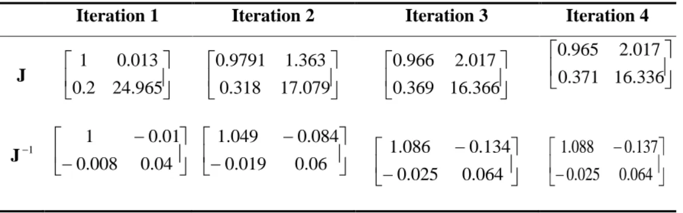
We found A0 18.905 million and A 32.87% with four iterations when starting with initial guess when A0 25and A 20%.The following tables, Table 2.3.A and Table 2.3.B, show the first four iterations of this

Table 2.3.A Results of Iterations

Iteration 1 Iteration 2 Iteration 3 Iteration 4

0 A 25 19.05 18.92 18.91 A  20% 28.78% 32.72% 32.87% 1 d 3.74 2.03 1.83 1.82 2 d 3.45 1.63 1.36 1.35 ) (d₁ N 0.9999 0.9789 0.9660 0.9654 ) (d₂ N 0.9997 0.9479 0.9135 0.9119 ) ( ₁ ' d N 0.0004 0.0506 0.0754 0.0765 Black-Scholes 15.9518 10.0680 10.0317 10.0000 g 5.95 0.068 0.0137 0 h -1.0005 -0.6334 -0.0184 0

Table 2.3.B Jacobian and Inverse Jacobian Matrix

Iteration 1 Iteration 2 Iteration 3 Iteration 4

J       965 . 24 2 . 0 013 . 0 1       079 . 17 318 . 0 363 . 1 9791 . 0       366 . 16 369 . 0 017 . 2 966 . 0 _      336 . 16 371 . 0 017 . 2 965 . 0 1  J         04 . 0 008 . 0 01 . 0 1         06 . 0 019 . 0 084 . 0 049 . 1         064 . 0 025 . 0 134 . 0 086 . 1         064 . 0 025 . 0 137 . 0 088 . 1

We can calculate the Merton bankruptcy of this company with the results from the fourth iteration. Probability of Default s equal toN(d2). This means, PD= 1

-)

2.4.2.1 Simplification of Distance to Default

The simplified expression contains only observable parameters and distance to default can be computed without solving nonlinear equations. The simplification is based on three assumptions.

1) AssumeN(d₁)is close to 1.

2) The limit of the drift term is equal to 0.

3) When calculating distance to default, use the book (face) value of debt instead of the leverage ratio.

T σ T σ )T σ 2 1 + (r + ) D / (A ln = T σ d = DD _A A 2 A T 0 A 1   T σ )T σ 2 1 (r + ) D / (A ln = DD A 2 A T 0 

Now, since the drift term is very small, close to the zero, than σ )T=0 2

1

(r ₂

A

 .

Rewrite the explanation of the volatility of the assets by using Ito’s Lemma, we found the following expression:

0 E 0 T 0 A T σ E ) D / (A ln = DD

Now assume time to maturity is equal to 1 year. So,

0 E 0 T 0 A σ E ) D / (A ln = DD . Since the

leverage ratio, which is denoted by L,

0 T A D = L . . A σ E (L) ln = A σ E ) D / (A ln = DD 0 E 0 0 E 0 T 0 

The DD is simply the number of standard deviations of a firm that is away from the default point within a specified time horizon. It is an ordinal measure of the firm’s

default risk. Chan-Lau and Say (2006) proposed the distance-to-capital as an alternative tool to forecasting bank default risk. The distance-to-capital is constructed the same way as the distance-to-default except that the default point is proposed as the capital thresholds, which is defined by the prompt-correction-action (PCA) frameworks. PCAs are typically rules-based frameworks, where rules are based on specific levels of a bank’s risk adjusted capital. The most commonly used capital threshold is the minimum capital adequacy ratio defined by the Basel II.

To determine the probability of default for a company, there are essentially three steps to be taken, as defined by Crosbie and Bohn (2003):

 Make an estimation of the asset value and the asset volatility30: In this step, estimation is made of the asset value and asset volatility of the firm based on the market value and volatility of equity and book value of liabilities.

 Calculate the distance to default31: The distance-to-default is calculated from the asset value and asset volatility and the book value of liabilities.

 Calculate the default probability: The default probability is a direct function of the distance-to-default.

The smaller DD, the larger the probability that the firm will default on its debt. It can be used to rank different firms according to their creditworthiness32. You can find more information about DD in appendix II.

30 _{The Black-Scholes model is used to calculate these values. Based upon the data collected, it is just}

matted of applying the formula like Löffler and Posch (2007) did to Enron (2001).

31

The distance-to-default is a function combined of several variables: value of assets, asset volatility and value of liabilities. But there is also another variable that is part of the distance-to-default: the asset drift rate. To calculate its value, the Capital Asset Pricing Model (CAPM) comes into the as a standard procedure for estimating expected returns.

32

In the literature one can sometimes see the risk free interest rate replaces with the asset value growth rate. The distance to default measure is then linked to real world default probabilities instead of risk neutral ones. Risk neutral probabilities are typically used for pricing purposes and real world probabilities for risk management purposes.

2.5 DEFAULT & SURVIVAL PROBABILITIES

According to the study of Paul Dunne and Alan Hughes, they shown smaller companies grew faster than larger companies, and age is negatively related to growth. In addition, their study shown that smaller companies had higher death rates but the largest and smallest companies was least vulnerable to takeover.33

What logically follows is that when the probability of default for company X is higher than for company Y, company X pays a higher interest on its debt than does company Y.

2.5.1 Bivariate Normal Distribution

Assume X and Y are two random variables with the following joint probability density function. y)) θ(x, ) ρ 1 ( 2 1 ( exp ρ 1 σ 2ΠΠ 1 = y) ψ(x, ₂ xy 2 Y X    , where 2 Y Y Y Y x x 2 x x σ μ y + σ μ y σ μ x 2 σ μ x = y) θ(x, _                             .

Then ψ(x,y)is known as the bivariate normal probability density function and is specified with five parameters; μ ,_X μ ,_Y σ ,_X σ and _Y ρ_X,Y, μ and _X μ is expectation _Y of the random variables X and Y, respectively. σ ,_X σ is standard deviation of the _Y random variables X and Y, respectively.ρ_X,Y is the correlation coefficient of X and Y. Knowing the default probability of each single party and joint default probability of both parties, we can obtain the default correlation. Evaluating default correlations or the probabilities of default by more than one firm is an important task in credit analysis, derivatives pricing, and risk management. However, default correlations can not be

33 _{Paul Dunne and Alan Hughes, “Age, Size, Growth and Survival”, UK Companies in the 1980s”, The} Journal of Industrial Economics, 1994.