Defining an Optimal Cut-Point Value in ROC Analysis: An Alternative Approach

(1)

Research Article

Defining an Optimal Cut-Point Value in ROC Analysis:

An Alternative Approach

Ilker Unal

School of Medicine, Department of Biostatistics, Cukurova University, Saricam, Adana, Turkey Correspondence should be addressed to Ilker Unal; [email protected]

Received 7 January 2017; Revised 5 April 2017; Accepted 7 May 2017; Published 31 May 2017 Academic Editor: Hiro Yoshida

Copyright © 2017 Ilker Unal. This is an open access article distributed under the Creative Commons Attribution License, which permits unrestricted use, distribution, and reproduction in any medium, provided the original work is properly cited.

ROC curve analysis is often applied to measure the diagnostic accuracy of a biomarker. The analysis results in two gains: diagnostic accuracy of the biomarker and the optimal cut-point value. There are many methods proposed in the literature to obtain the optimal cut-point value. In this study, a new approach, alternative to these methods, is proposed. The proposed approach is based on the value of the area under the ROC curve. This method defines the optimal cut-point value as the value whose sensitivity and specificity are the closest to the value of the area under the ROC curve and the absolute value of the difference between the sensitivity and specificity values is minimum. This approach is very practical. In this study, the results of the proposed method are compared with those of the standard approaches, by using simulated data with different distribution and homogeneity conditions as well as a real data. According to the simulation results, the use of the proposed method is advised for finding the true cut-point.

1. Introduction

The ROC curve is a mapping of the sensitivity versus 1 −

specificity for all possible values of the cut-point between cases and controls. To measure the diagnostic ability of a biomarker, it is common to use summary measures such as the area under the ROC curve (AUC) and/or the partial area under the ROC curve (pAUC) [1]. A biomarker with AUC = 1 discriminates individuals perfectly as diseased or healthy. Meanwhile, an AUC = 0.5 means that there is no apparent distributional difference between the biomarker values of the two groups [2].

ROC analysis provides two main outcomes: the diagnos-tic accuracy of the test and the optimal cut-point value for the test. Cut-points dichotomize the test values, so this provides the diagnosis (diseased or not). The identification of the cut-point value requires a simultaneous assessment of sensitivity and specificity [3]. A cut-point will be referred to as optimal when the point classifies most of the individuals correctly [4, 5].

AUC, sensitivity, and specificity values are useful for the evaluation of a marker; however they do not specify “optimal” cut-points directly. In the literature, related to the subject, there are many approaches using both sensitivity

and specificity for cut-point selection [4–9]. One of the commonly used method is the Youden index (𝐽) method [5]. This method defines the optimal cut-point as the point maximizing the Youden function which is the difference between true positive rate and false positive rate over all possible cut-point values [6, 7]. Another approach is known as the point closest-to-(0, 1) corner in the ROC plane (ER) which defines the optimal cut-point as the point minimizing the Euclidean distance between the ROC curve and the (0, 1) point [4]. A third approach is based on the maximum

achievable value of the chi-square statistic (min𝑃) which is

driven using the cross-tabulations of true disease status and categorized new variables that separate the biomarker into two categories according to all possible cut-point values [8]. A more recent approach was proposed by Liu [9], which defines the optimal cut-point as the point maximizing the product of sensitivity and specificity (CZ). In the literature, there are studies comparing optimal metrics derived from the sensitivity, specificity, agreement, and distance [10, 11]. In these studies, it is generally recommended that researchers should select one that is most clinically relevant.

In this study, a new approach is proposed for the identi-fication of the optimal cut-point value in ROC analysis. The approach is based on the area under the ROC curve (AUC), Volume 2017, Article ID 3762651, 14 pages

(2)

sensitivity, and specificity values. It defines the optimal cut-point value as the cut-point minimizing the summation of abso-lute values of the differences between AUC and sensitivity and AUC and specificity provided that the difference between sensitivity and specificity is minimum.

In the following section, first the background method-ologies of previous methods are summarized, and, then, the proposed method is introduced. In Section 3, in order to compare the performance of the previous methods with that of the proposed one, generated data under the assumption of normal distribution and gamma distribution models for the biomarker are used. Then, in Section 4, using data from a real-world study of heart-failure patients [12], the cut-points for pulse pressure, plasma sodium, LVEF, and heart rate in prediction of mortality are calculated by applying the proposed and the previous methods. Finally, in Section 5, conclusions are given.

2. Previous Methods and the Proposed Method

2.1. Minimum𝑃 Value Approach (min 𝑃). Let 𝑋 be a

contin-uous biomarker that is assumed to be predictive of an event

𝐸 (i.e., 𝐸 = 1 for diseased or 𝐸 = 0 for not diseased). At any

given possible cut-point𝑐 of 𝑋, sensitivity (Se) and specificity

(Sp) values are as follows:

Se(𝑐) = 𝑃 (𝑋 > 𝑐 | 𝐸 = 1) ,

Sp(𝑐) = 𝑃 (𝑋 ≤ 𝑐 | 𝐸 = 0) . (1)

Cut-point𝑐 separates the data into two groups which forms a

2 × 2 table, as shown in Table 1.

The minimum𝑃 value approach was proposed by Miller

and Siegmund [8] and defines the optimal point as cut-point ̂𝑐min 𝑃that maximizes the standard chi-square statistic with

one degree of freedom:

𝜒2

1(𝑐) = 𝑁 (𝑠V − 𝑢𝑟)

2

(𝑠 + 𝑟) (𝑢 + V) (𝑠 + 𝑢) (𝑟 + V), (2)

where 𝑁 = 𝑠 + 𝑟 + 𝑢 + V. As it was shown by Rota and

Antolini [11], it can be also written in terms of classification probabilities:

𝜒2₁(𝑐) = (Se (𝑐) + Sp (𝑐) − 1)

2

(((𝑢 + V) Se (𝑐) + (𝑠 + 𝑟) (1 − Sp (𝑐))) /𝑁) (1 − ((𝑢 + V) Se (𝑐) + (𝑠 + 𝑟) (1 − Sp (𝑐))) /𝑁) (1/ (𝑢 + V) + 1/ (𝑠 + 𝑟)). (3)

2.2. Youden Index(𝐽). The Youden index (𝐽) is a measure

for evaluating the biomarker effectiveness. This measure was

first introduced to the medical literature by Youden [5].𝐽 is a

function of Se(𝑐) and Sp(𝑐), such that

𝐽 (𝑐) = {Se (𝑐) + Sp (𝑐) − 1} = {Se (𝑐) − (1 − Sp (𝑐))} (4)

over all cut-points𝑐; ̂𝑐_𝐽denotes the cut-point corresponding

to𝐽. When the value of 𝐽 is maximum, ̂𝑐_𝐽is the “optimal”

cut-point value [6, 7].

2.3. The Closest to (0, 1) Criteria (ER). In this criteria, the

“optimal” cut-point is defined as the point closest to the point (0, 1) on the ROC curve [3, 4].

ER(𝑐) = (√(1 − Se (𝑐))2+ (1 − Sp (𝑐))2) . (5)

Mathematically, the point̂𝑐_ERminimizing the ER(𝑐) function

is called the “optimal” cut-point value.

2.4. Concordance Probability Method (CZ). The concordance

probability method proposed by Liu [9] defines the optimal cut-point as the point maximizing the product of sensitivity and specificity.

CZ(𝑐) = Se (𝑐) ∗ Sp (𝑐) . (6)

This product gets value between 0 and 1. The concordance

probability of dichotomized measure at cut-point𝑐 can be

expressed as the area of a rectangle associated with the ROC

curve. Cut-point̂𝑐_CZ maximizing CZ(𝑐) actually maximizes

the area of the rectangle [9].

2.5. The Proposed Method: Index of Union (IU). Perkins and

Schisterman [4] stated that the “optimal” cut-point should be chosen as the point which classifies most of the individuals correctly and thus least of them incorrectly. From this point of view, in this study, the Index of Union method is proposed. This method provides an “optimal” cut-point which has maximum sensitivity and specificity values at the same time. In order to find the highest sensitivity and specificity values at the same time, the AUC value is taken as the starting value of them. For example, let AUC value be 0.8. The next step is to look for a cut-point from the coordinates of ROC whose sensitivity and specificity values are simultaneously so close or equal to 0.8. This cut-point is then defined as the “optimal” cut-point. The above criteria correspond to the following equation:

IU(𝑐) = (|Se (𝑐) − AUC| + 󵄨󵄨󵄨󵄨Sp (𝑐) − AUC󵄨󵄨󵄨󵄨). (7)

The cut-point̂𝑐_IU, which minimizes the IU(𝑐) function and

the|Se(𝑐) − Sp(𝑐)| difference, will be the “optimal” cut-point

value.

In other words, the cut-point ̂𝑐_IU defined by the IU

method should satisfy two conditions: (1) sensitivity and specificity obtained at this cut-point should be simultane-ously close to the AUC value; (2) the difference between sensitivity and specificity obtained at this cut-point should be minimum. The second condition is not compulsory, but it is an essential condition when multiple cut-points satisfy the equation.

In order to illustrate how the IU method defines the “optimal” cut-point, the values obtained from an artificial

(3)

Table 1

𝑋 ≤ 𝑐 𝑋 > 𝑐

𝐸 = 0 𝑠 𝑟

𝐸 = 1 𝑢 V

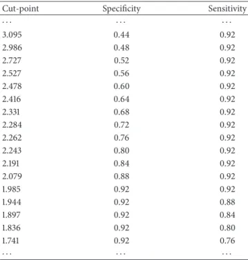
Table 2: Some of the cut-points with their sensitivity and specificity values obtained from artificial data.

Cut-point Specificity Sensitivity

⋅ ⋅ ⋅ ⋅ ⋅ ⋅ ⋅ ⋅ ⋅ 3.095 0.44 0.92 2.986 0.48 0.92 2.727 0.52 0.92 2.527 0.56 0.92 2.478 0.60 0.92 2.416 0.64 0.92 2.331 0.68 0.92 2.284 0.72 0.92 2.262 0.76 0.92 2.243 0.80 0.92 2.191 0.84 0.92 2.079 0.88 0.92 1.985 0.92 0.92 1.944 0.92 0.88 1.897 0.92 0.84 1.836 0.92 0.80 1.741 0.92 0.76 ⋅ ⋅ ⋅ ⋅ ⋅ ⋅ ⋅ ⋅ ⋅

data are used. Some of the cut-points (with their sensitivity and specificity values) provided by the artificial data are given in Table 2. In this example, the AUC value is calculated as

0.918. For the sake of simplicity, instead of 1 − specificity

values, specificity values are given in the table. By using IU method, one can easily find that sensitivity (0.92) and specificity (0.92) values of the cut-point 1.985 are the nearest ones to the AUC value. Since also the difference between these two values is minimum, this cut-point will be called the “optimal” cut-point by the IU method.

However, it should be noted that choosing such a cut-point as the “optimal” cut-cut-point may sometimes fail. For example, let Se(𝑐) = Sp(𝑐) = AUC = 0.8. Then, the IU(𝑐) statistic given in (7) will be 0 and also the difference between Se(𝑐) and Sp(𝑐) will be 0. Thus according to the definition

of optimality given in the IU method, cut-point 𝑐 will be

accepted as the “optimal” cut-point. However, if there is a

point𝑐∗for which Se(𝑐∗) = 0.82 and Sp(𝑐∗) = 0.80, then the

total misclassification rate will be 0.38 (which is smaller than

that of the point𝑐, i.e., 0.40). Hence, cut-point 𝑐∗is a better

optimized point than cut-point𝑐, based on the definition of

optimality given by Perkins and Schisterman [4].

Geometrically, the idea behind the IU method is very similar to the idea behind the ER method. As it can be seen in Figure 1, the IU method also tries to find the closest point to a point, that is, the point (1 − AUC, AUC). In the ER

ROC curve 0.892 AUC = 0.892 A B D C 0,0 0,2 0,4 0,6 0,8 1,0 Se ns itiv ity x = 1 − Sp(cIU) = 0.203 x = 1 − AUC = 0.108 y = Se(cIU) = 0.837 y = AUC = 0.892 0,6 0,2 0,4 0,8 1,0 0,0 1 − specificity

Figure 1: The receiver operator characteristic curve for pulse pressure in the prediction of cardiovascular death [12].

method, this point is taken as (0, 1). However, instead of

using the Euclidean distance as in the ER method, the IU method uses the absolute differences between the diagnostic accuracy measures and the AUC value. More specifically, the IU method searches for the point that minimizes the half perimeter of the ABCD rectangle seen in Figure 1. This rectangle is constructed by connecting the intersections

points of the lines of𝑥 = 1 − AUC, 𝑦 = AUC, 𝑥 = 1 − Sp(𝑐),

and𝑦 = Se(𝑐).

3. Simulation Study

As it was shown by Rota and Antolini [11] although some of these methods are mathematically related, they do not nec-essarily identify the same true cut-point. That is, depending on the design of the study (balanced or unbalanced), the methods may identify different cut-points. According to their results, in the balanced homoscedastic scenario, the methods identified the same point; in the remaining scenarios (i.e., unbalanced homoscedastic and balanced/unbalanced het-eroscedastic scenarios), the methods identified different cut-points. These results emphasize the importance of correctly defining the true cut-point in all possible scenarios.

Let us assume that a specific biomarker (𝑋) in diseased

and nondiseased populations is normally distributed,𝑋₁ ∼

𝑁 (𝜇₁, 𝜎₁= 1) for diseased subjects and 𝑋₀∼ 𝑁 (0, 𝜎₀= 1)

for nondiseased subjects. Under these assumptions, sensitiv-ity and specificsensitiv-ity can be written as

Se(𝑐) = 𝑃 (𝑋₁≥ 𝑐) = Φ (𝜇₁− 𝑐) ,

Sp(𝑐) = 𝑃 (𝑋₀≤ 𝑐) = Φ (𝑐) , (8)

whereΦ denotes the standard normal distribution function.

(4)

5 10 15 20 25 0 x 0 20 40 60 80 100 c cIUIU= 1.42= 1.78 c cIUIU= 2.41= 3.30

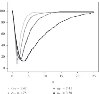
Figure 2: The empirically estimated objective functions IU(𝑐) under different underlying distributions: light to dark colors represent the scenarios with the classification accuracies from poor to high one. The homoscedastic gamma distribution scenario with a balanced design (𝑛₀= 𝑛₁= 100) is represented.

probability density functions of diseased and nondiseased

subjects (i.e.,𝑐_opt = 𝜇₁/2) [7, 13]. For example, if 𝜇₁is taken

as{0.51, 1.05, 1.68, 2.56}, the corresponding true cut-points

will be𝑐_opt= {0.25, 0.52, 0.84, 1.28} [11, 13]. These values of 𝜇₁

guarantee a wide variety of classification accuracies, ranging from a poor to a high one [7, 11, 13]. The identification of the true theoretical cut-point for the IU method under this scenario is given in the Appendix.

Now assume that𝑋 is gamma distributed with the

follow-ing parameters:𝑋₁ ∼ 𝐺 (𝛼₁ = 2.5, 𝛽₁) for diseased subjects

and𝑋₀ ∼ 𝐺 (𝛼₀ = 1.5, 𝛽₀ = 1) for nondiseased subjects. If,

for instance,𝛽₁is taken as{0.79, 1.22, 1.97, 3.82}, the

corre-sponding cut-points for each method will be different; that

is, for min𝑃 approach, 𝑐_{min 𝑃} = {0.80, 1.73, 2.54, 3.51}, for

Youden index,𝑐_𝐽 = {1.12, 1.79, 2.45, 3.42}, for the

concor-dance probability,𝑐_CZ = {1.35, 1.81, 2.41, 3.38}, and, for the

point closest-to-(0, 1) corner, 𝑐_ER = {1.38, 1.82, 2.36, 3.24}

[11]. For the Index of Union, the corresponding cut-points are estimated by the empirical estimation method given in Liu’s

work [9] as𝑐_IU= {1.42, 1.78, 2.41, 3.30} (Figure 2).

In order to compare the performance of the cut-point selection methods with the performance of the method proposed in this study, a simulation study is conducted with different scenarios. These scenarios are the same as the ones given in Rota and Antolini’s work [11]. The first scenario is normal homoscedastic scenario with balanced design where all of the methods theoretically identify the same true cut-point. The second one is the nonbalanced normal case, where

all of the methods except the min𝑃 approach identify the

same cut-point. The last scenario is gamma case where all of the methods identify different cut-points.

In all scenarios, 1000 samples were generated with sample sizes 50, 100, and 200 for each group and with sample size

𝑛1 = 50, 𝑛0= 100; 𝑛1 = 50, 𝑛0 = 150; and 𝑛1 = 50, 𝑛0 = 200

(𝑛₁is the number of diseased subjects and𝑛₀is the number

of nondiseased subjects).

For each sample, the optimal cut-pointŝ𝑐_{min 𝑃},̂𝑐_𝐽,̂𝑐_CZ,̂𝑐_ER,

and̂𝑐_IUfor the minimum𝑃 value, the Youden index, the

con-cordance probability, the point closest-to-(0, 1) corner, and the Index of Union are estimated, respectively. The relative bias and mean square error (MSE) values of each method

are computed by𝐸[(̂𝑐 − 𝑐)/𝑐] and 𝐸[(̂𝑐 − 𝑐)2], respectively. (𝑐

denotes the true cut-point and̂𝑐 denotes the estimated

cut-point by the method.)

In order to estimate the standard deviation and the confidence interval (CI) for the optimal cut-point, the boot-strap resampling technique is applied [14]. To calculate the

bootstrap estimate ̂𝑐_𝐵, random sampling with replacement

is used to draw 200 bootstrap samples within each of the 1000 generated samples. Moreover, to construct a 95% CI for the optimal cut-point, the basic percentile method is applied

by taking the 2.5 and 97.5 percentiles of the ̂𝑐_𝐵 bootstrap

distribution.

The bootstrap estimator of the standard deviation (SD_𝐵)

for the estimated cut-point is calculated by taking the stan-dard deviation of the 200 cut-point estimates. Within each of the simulation scenarios, the CIs are subsequently evaluated by computing coverage probability and mean length.

All simulations are done by using R program with the version of 3.2.0. To determine the estimates for Youden index and the point closest-to-(0, 1) corner, the pROC library is used [15]. For defining the estimates of the rest of the methods, an R code is written by the author and it can be available upon request.

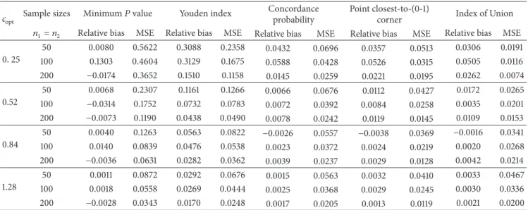
3.1. Simulation Results. Table 3 shows the results for the

balanced design under normal homoscedastic distributions. The relative bias values of the previously proposed methods are similar to the results of Rota and Antolini’s work [11] except the relative bias of Youden index. In particular for

poor classification accuracy scenarios (i.e.,𝑐_opt = 0.25 and

0.52), Youden index has worse performance in the estimation of the optimal cut-point than their results. However, this discrepancy is not seen in the comparison of MSEs. That is, the MSEs of all methods are similar to that of Rota and Antolini’s work [11].

When comparing the relative bias and MSE values of the IU method with that of the other methods, it can be easily seen that the IU method has mostly similar performance with the point closest-to-(0, 1) corner method and has better performance than the other methods (i.e., lower relative bias and lower MSE values).

For the balanced design under normal homoscedastic distributions, the bootstrap standard deviation, coverage probability, and mean length of the 95% bootstrap CI for the cut-point are shown in Table 4. As in Table 3, the results given in Table 4 are similar to that of Rota and Antolini’s work

[11]. That is, the SD_𝐵of the minimum𝑃 value approach is

still greater with respect to that of the other methods and the better classification accuracies provide the narrower 95%

bootstrap CIs. The IU method achieves the smallest SD_𝐵value

and the narrowest CIs in most of the scenarios. The coverage probabilities are close to the nominal level for all methods.

(5)

Table 3: Relative bias and mean square error (MSE) of all methods. The normal homoscedastic balanced scenarioa.

𝑐opt Sample sizes Minimum𝑃 value Youden index

Concordance probability

Point closest-to-(0-1)

corner Index of Union

𝑛1= 𝑛2 Relative bias MSE Relative bias MSE Relative bias MSE Relative bias MSE Relative bias MSE

0. 25 50 0.0080 0.5622 0.3088 0.2358 0.0432 0.0696 0.0357 0.0513 0.0306 0.0191 100 0.1303 0.4604 0.3129 0.1675 0.0588 0.0428 0.0526 0.0315 0.0505 0.0116 200 −0.0174 0.3652 0.1510 0.1158 0.0145 0.0259 0.0221 0.0195 0.0262 0.0074 0.52 50 0.0068 0.2307 0.1161 0.1266 0.0066 0.0676 0.0112 0.0427 0.0172 0.0265 100 −0.0314 0.1752 0.0732 0.0783 0.0072 0.0392 0.0084 0.0258 0.0035 0.0201 200 −0.0073 0.1190 0.0438 0.0490 0.0078 0.0242 0.0119 0.0145 0.0109 0.0153 0.84 50 0.0040 0.1263 0.0563 0.0822 −0.0026 0.0557 −0.0038 0.0369 −0.0016 0.0341 100 0.0140 0.0839 0.0476 0.0538 0.0023 0.0372 0.0024 0.0219 0.0020 0.0268 200 −0.0036 0.0631 0.0282 0.0362 0.0039 0.0237 0.0029 0.0128 0.0042 0.0214 1.28 50 0.0011 0.0872 0.0292 0.0676 0.0015 0.0563 0.0032 0.0410 0.0033 0.0467 100 0.0018 0.0558 0.0269 0.0444 0.0025 0.0368 0.0029 0.0245 0.0030 0.0336 200 −0.0028 0.0343 0.0170 0.0248 0.0017 0.0205 0.0013 0.0119 0.0021 0.0200 a_𝑋

1∼ 𝑁 (𝜇1, 1), 𝑋0∼ 𝑁 (0, 1), and 𝜇1was taken as 0.51, 1.05, 1.68, and 2.56, respectively.

The relative bias and MSE results for the unbalanced design under normal homoscedastic distributions are shown

in Table 5. Since the true cut-point for the minimum 𝑃

value approach depends on the prevalence of the disease in the sample, different optimal cut-points are used for the comparisons [11]. The relative bias values of all methods are similar to those of Rota and Antolini’s work [11], except for

the minimum𝑃 value approach in the lowest classification

accuracy scenario (i.e.,𝑐_opt = 0.25). For this scenario the

relative bias for the minimum𝑃 value approach is larger than

the bias given in their work. For poor and poor-moderate

classification accuracy (i.e.,𝑐_opt = 0.25 and 0.52), the MSE

is the lowest for the IU method, and, for moderate-high and

high classification accuracy (i.e.,𝑐_opt = 0.84 and 1.28), both

the point closest-to-(0, 1) corner method and the IU method get the lowest MSE values.

For the unbalanced design under normal homoscedastic distributions, the bootstrap standard deviation, coverage probability, and mean length of the 95% bootstrap CI for the cut-point are given in Table 6. For this scenario, the lowest

SD_𝐵 and mean length of the 95% bootstrap CI values are

obtained by the point closest-to-(0, 1) corner method and the IU method. As in the comparison of the relative bias and MSE values of the methods (Table 5), for poor and

poor-moderate classification accuracy (i.e.,𝑐_opt = 0.25 and 0.52),

the IU method gets the lowest SD_𝐵and mean length, and, for

moderate-high and high classification accuracy (i.e.,𝑐_opt =

0.84 and 1.28), both the point closest-to-(0, 1) corner in the ROC plane and the IU method get the lowest values. The coverage probabilities are close to the nominal level for all methods.

As it was shown in Rota and Antolini’s work [11], under a gamma distribution assumption with a balanced design,

the theoretical true cut-points 𝑐_{min 𝑃}, 𝑐_𝐽, 𝑐_CZ, and 𝑐_ER are

all different. For all classification accuracy scenarios, the theoretical true cut-points for the IU method are obtained based on the idea given in the article of Liu [9] (Figure 2).

The relative bias values of all methods are similar to those of Rota and Antolini’s work [11]. The MSE gets its lowest value in the point closest-to-(0, 1) corner and the IU method for all classification accuracy scenarios (Table 7).

For this design (under gamma distributions), the SD_𝐵and

mean length of 95% CI values for the point closest-to-(0, 1) corner method and the IU method are lower than the other investigated approaches (Table 8). The coverage probabilities are close to the nominal level for all methods.

In all simulation scenarios, the IU method shows a better performance in the estimation of the optimal cut-point with respect to the other methods. The bootstrap standard deviation and mean length of the 95% bootstrap CI values for the IU method are also minimum among all methods. Thus, for all simulation scenarios, although, in gamma scenarios, the methods do not lead to a common cut-point, in order to identify the optimal cut-point, the IU method is a better alternative than the previous proposed methods.

3.2. Cross-Validation of the Optimal Cut-Point. In order to

evaluate the significance of the optimally selected cut-point, twofold cross-validation process [16] is used. The procedure is as follows:

(1) Generating data with the same properties given in this manuscript

(2) Applying all methods to the data and estimating cut-points for all methods

(3) Splitting data into two equal subsets, that is, subset I and subset II

(4) Applying all methods to subset I and estimating cut-points for all methods

(5) Assigning each observation in subset II to either one of two groups by using the cut-point obtained in the previous step

(6)

T a ble 4: B o o tst ra p st an da rd de via tio n, co vera ge p ro b ab ili ty ,a n d m ea n len gt h o f the 95% co nfidence in ter val est ima tio n o f all met h o d s. The no rm al ho mo sc edast ic b ala n ced scena rio a . 𝑐opt Sa m p le sizes M inim um 𝑃 va lu e Y o uden index C o nco rd ance p ro b ab ili ty P o in t clos est-t o-(0-1) co rn er In dex o f U nio n 𝑛1 =𝑛 2 SD 𝐵 C o ve ra ge M ean le ng th SD 𝐵 C o ve ra ge M ean le ng th SD 𝐵 C o ve ra ge M ean le ng th SD 𝐵 C o ve ra ge Me an len gt h SD 𝐵 C o ve ra ge M ean le ng th 0.2 5 50 0.7 47 3 0.9 6 4 2.7 55 9 0.47 76 0.9 69 1.8 4 84 0.26 33 0.97 1 1.0 33 3 0.226 2 0.9 69 0.88 37 0.13 80 0.97 4 0.5 50 2 10 0 0.67 67 0.9 67 2.5 63 7 0.4 01 7 0.9 6 8 1.5 55 3 0.20 61 0.97 3 0.807 4 0.1 76 7 0.97 2 0.7 01 9 0.107 0 0.9 6 6 0.41 73 20 0 0.6 03 9 0.9 6 8 2.3 05 9 0.3 38 0.9 69 1.3 0 63 0.16 0 6 0.95 9 0.58 9 6 0.13 93 0.9 67 0.5 35 9 0.08 58 0.97 0 0 .3 32 5 0.5 2 50 0.4 81 1 0.9 6 8 1.8 521 0.3 507 0.9 69 1.3 411 0.26 02 0.97 1 1.018 1 0.207 1 0.97 3 0.8187 0.16 30 0 .97 3 0.6 47 6 10 0 0.4186 0.9 6 8 1.587 8 0.2 77 8 0.97 2 1.10 0 6 0.1 98 2 0.9 69 0.7 56 6 0.16 07 0.97 0 0.6 23 3 0.1 4 20 0.9 69 0.5 4 89 20 0 0.3 43 4 0.97 0 1.3 39 9 0.21 9 0.97 5 0.87 86 0.15 51 0.97 3 0.6 13 9 0.11 9 9 0.97 1 0.47 17 0.12 31 0.9 65 0.4 62 3 0.8 4 50 0.3 55 6 0.9 69 1.3 557 0.2 826 0.9 69 1.08 37 0.2 35 4 0.97 3 0.9 26 1 0.1 92 1 0.97 4 0.7 69 2 0.18 45 0.97 6 0.7 47 5 10 0 0.2 89 9 0.97 0 1.110 6 0.22 89 0.97 2 0.8 92 2 0.1 93 0 0.97 2 0.7 59 5 0.1 47 7 0.97 2 0.58 43 0.16 37 0.97 0 0.6 49 1 20 0 0.2 515 0.97 0 0.9 61 9 0.18 9 0 0.97 2 0.7 37 5 0.15 38 0.97 5 0.6 15 4 0.113 2 0.97 1 0.4 35 6 0.1 4 65 0.97 0 0.5 6 01 1.2 8 50 0.2958 0.9 65 1.110 6 0.2 57 8 0.97 4 1.0 26 2 0.2 37 9 0.97 4 0.941 9 0.20 27 0.97 3 0.81 98 0.216 6 0.97 4 0.86 6 8 10 0 0.2 35 9 0.9 6 8 0.8 97 3 0.207 4 0.97 2 0.8112 0.1 91 6 0.97 5 0.7 679 0.15 6 6 0.97 1 0.6 157 0.18 31 0.97 3 0 .7 294 20 0 0.18 51 0.97 1 0.7 24 0 0.15 56 0.97 0 0.6 141 0.1 43 1 0.97 0 0.5 6 83 0.10 94 0.97 2 0.4 27 2 0.1 41 4 0.9 69 0.5 6 07 a 𝑋 1 ∼𝑁 (𝜇1 ,1 ), 𝑋0 ∼𝑁 (0, 1) ,a n d 𝜇1 w ast ak ena s0 .5 1,1 .0 5,1 .6 8,a n d2 .5 6 ,r es p ec ti ve ly .

(7)

T a ble 5: R ela ti ve b ias and me an sq ua re er ro r (MS E) o f al lm et ho ds. Th e n o rma lh o m os cedast ic un b ala nced scena rio a . 𝑐opt 𝑐min 𝑃 Sa m p le sizes M inim um 𝑃 val ue Y o uden index C o nco rd ance pro b abi lit y P o in t clos est-t o-(0-1) co rn er In dex o f U nio n 𝑛1 𝑛2 Re la ti ve b ia s MS E Re la ti ve b ia s M SE Re la ti ve b ia s MS E Re la ti ve b ia s M SE Re la ti ve b ia s MS E 0.2 5 0.3 9 50 10 0 0.1 75 0 0.5 0 41 0.20 4 6 0.18 13 0.10 4 2 0.05 20 0.10 07 0.0 341 0.0 6 86 0.0 07 5 0.4 6 50 150 0.2986 0.5 12 4 0.16 83 0.1 70 8 0.11 4 2 0.05 15 0.13 24 0.0 33 8 0.0 92 3 0.0 079 0.5 1 50 20 0 0.295 5 0.5 51 7 0.1 4 20 0.1 74 1 0.1 4 83 0.0 4 84 0.15 4 4 0.0 32 0 0.105 9 0.0 07 4 0.5 2 0.7 5 50 10 0 0.0 36 1 0.1 9 63 0.10 61 0.0 92 1 0.057 2 0.0 4 69 0.0 4 81 0.0 25 6 0.05 35 0.016 1 0.87 50 150 0.0 613 0.1 92 2 0.11 41 0.0 9 0 4 0.0588 0.0 43 5 0.07 4 6 0.0 25 5 0.05 97 0.016 2 0.9 6 50 20 0 0.0 6 01 0.20 6 0 0.0 92 6 0.07 85 0.0 69 0 0.0 39 9 0.07 78 0.0 23 3 0.0 69 6 0.015 9 0.8 4 1.0 9 50 10 0 0.0 0 0 6 0.0 95 2 0.0 411 0.05 97 0.0157 0.0 41 4 0.0 21 9 0.0 21 9 0.016 2 0.0 25 5 1.2 3 50 150 0.0 03 0 0.0 95 6 0.0 498 0.0580 0.0 313 0.0 4 23 0.0 37 5 0.0 23 2 0.0 32 8 0.0 25 9 1.3 3 50 20 0 0.0 02 8 0.0 9 9 6 0.0 4 4 0 0.05 36 0.0 34 5 0.0 37 4 0.0 4 0 9 0.0 201 0.0 34 2 0.0 24 8 1.2 8 1.5 0 50 10 0 −0.0123 0.058 1 0.0 35 0 0.0 4 6 0 0.01 77 0.0 39 0 0.0 22 5 0.0 25 4 0.01 95 0.0 32 5 1.6 3 50 150 −0.0055 0.05 28 0.0 37 8 0.0 479 0.0 25 4 0.0 41 4 0.0 298 0.0 24 2 0.0 27 0 0.0 34 2 1.7 2 50 20 0 0.0 0 0 7 0.05 07 0.0 4 69 0.0 47 7 0.0 38 0 0.0 4 22 0.0 38 6 0.0 257 0.0 36 8 0.0 35 6 a𝑋 1 ∼𝑁 (𝜇1 ,1 ), 𝑋0 ∼𝑁 (0, 1) ,a n d 𝜇1 w ast ak ena s0 .5 1,1 .0 5,1 .6 8,a n d2 .5 6 ,r es p ec ti ve ly .

(8)

T a ble 6: B o o tst ra p st an da rd de via tio n, co vera ge p ro b ab ili ty ,a n d m ea n len gt h o f the 95% co nfidence in ter val est ima tio n o f all met h o d s. The no rm al ho mo sc edast ic u n b ala n ced scena rio a . 𝑐opt 𝑐min 𝑃 Sa m p le sizes M inim um 𝑃 val ue Y o uden index C o nco rda nce p ro ba b ili ty P o in t clos est-t o-(0-1) co rn er In dex o f U nio n 𝑛1 𝑛2 SD 𝐵 C o ve ra ge Me an len gt h SD 𝐵 C o ve ra ge Me an len gt h SD 𝐵 C o ve ra ge Me an len gt h SD 𝐵 C o ve ra ge Me an len gt h SD 𝐵 C o ve ra ge Me an len gt h 0.2 5 0.3 9 50 10 0 0.6 9 6 8 0.9 6 8 2.6 36 5 0.4 205 0.9 69 1.6 05 9 0.229 6 0.9 6 8 0.8881 0.18 51 0.97 1 0.7 19 1 0.087 4 0.9 67 0.3 50 4 0.4 6 50 150 0.7 02 7 0.9 62 2.6 012 0.4108 0.9 69 1.6 012 0.22 47 0.9 67 0.87 51 0.180 4 0.9 67 0.6 89 2 0.08 56 0.9 6 4 0 .333 6 0.5 1 50 20 0 0.7 27 7 0.9 6 0 2.6 87 1 0.4157 0.97 2 1.6 15 1 0.21 71 0.9 67 0.8 51 4 0.1 74 7 0.9 6 4 0.6 63 3 0.08 21 0.95 9 0.3 17 4 0.5 2 0.7 5 50 10 0 0.4 41 9 0.97 1 1.7 011 0.298 3 0.9 69 1.1 4 61 0.215 1 0.9 69 0.8 25 2 0.157 6 0.9 67 0.6 0 6 8 0.12 34 0 .9 67 0.4 6 6 6 0.87 50 150 0.4 34 0 0.97 1 1.6 81 6 0.294 3 0.9 6 6 1.1 4 59 0.20 61 0.97 1 0.80 03 0.15 4 8 0.97 5 0.6 226 0.12 31 0 .9 61 0.4 67 1 0.9 6 50 20 0 0.45 0 4 0.9 6 8 1.7 34 6 0.2 757 0.9 6 6 1.0 6 01 0.1 9 6 4 0.97 1 0.7 88 2 0.1 47 0 0.9 67 0.5 6 85 0.1207 0.9 6 8 0.45 61 0.8 4 1.0 9 50 10 0 0.3 08 1 0.97 0 1.1 86 6 0.2 416 0.97 1 0.9 34 3 0.20 31 0.97 1 0.80 28 0.1 47 2 0.97 0 0.57 54 0.15 94 0.9 67 0.6 03 1 1.2 3 50 150 0.3 0 94 0.97 1 1.20 33 0.2 37 5 0.97 0 0.9 12 3 0.20 4 4 0.97 3 0.80 6 4 0.1 4 89 0.97 1 0.5805 0.158 5 0 .9 69 0 .600 1 1.3 3 50 20 0 0.3 15 1 0.9 69 1.226 5 0.229 2 0.97 2 0.8 91 7 0.1 91 4 0.97 2 0.7 63 9 0.13 79 0.9 6 8 0.5 26 1 0.15 47 0.9 6 4 0.5 6 4 8 1.2 8 1.5 0 50 10 0 0.2 4 0 8 0.9 6 8 0.9 19 9 0.20 92 0.97 2 0.8 294 0.1 95 5 0.97 4 0.7 84 6 0.15 63 0.97 1 0.6 0 93 0.1 78 0 0.97 2 0.6 941 1.6 3 50 150 0.2298 0.97 3 0.9 08 9 0.213 1 0.97 2 0.8 4 23 0.20 0 4 0.97 2 0.798 3 0.15 0 6 0.97 3 0.5 9 62 0.18 18 0.97 0 0.7 011 1.7 2 50 20 0 0.22 54 0.9 6 8 0.87 16 0.2101 0.9 6 6 0.80 9 6 0.1 9 98 0.9 6 4 0.7 67 1 0.15 26 0.97 0 0.5 929 0.18 25 0.9 65 0.6 89 0 a 𝑋 1 ∼𝑁 (𝜇1 ,1 ), 𝑋0 ∼𝑁 (0, 1) ,a n d 𝜇1 w ast ak ena s0 .5 1,1 .0 5,1 .6 8,a n d2 .5 6 ,r es p ec ti ve ly .

(9)

T a ble 7: R el at ive b ia s and me an sq u ar e er ro r (MS E) o f al lm et ho ds. Th e ga m ma b al ance d scena rio a . 𝑐min 𝑃 𝑐𝐽 𝑐CZ 𝑐ER 𝑐IU Sa m p le sizes M inim um 𝑃 va lu e Y o uden index C o nco rd ance p ro b ab ili ty P o in t clos est-t o-(0-1) co rn er In dex o f U nio n 𝑛1 =𝑛 2 Re la ti ve b ia s MS E Re la ti ve b ia s M SE Re la ti ve b ia s MS E Re la ti ve b ia s MS E Re la ti ve b ia s MS E 0.80 1.12 1.3 5 1.3 8 1.4 2 50 0.4 29 0 0.5 49 1 0.086 2 0.20 95 0.01 74 0.07 13 0.010 0 0.05 21 0.0 24 3 0.013 3 10 0 0.2 73 5 0.3 0 01 0.05 65 0.13 21 0.0126 0.0 4 6 4 0.0 016 0.0 31 4 0.01 95 0.0 07 8 20 0 0.1 93 4 0.18 13 0.0 39 5 0.088 5 0.0116 0.0 305 0.0 02 4 0 .0 211 0.015 6 0.0 0 65 1.7 3 1.79 1.8 1 1.8 2 1.7 8 50 0.07 35 0.47 27 0.0 26 9 0.226 0 0.016 8 0.1108 0.016 0 0 .0 6 4 8 0.0 36 5 0.0 4 01 10 0 0.0 45 4 0.3 34 7 0.0 229 0.13 28 0.0 0 9 9 0.0 65 5 0.0126 0.0 38 5 0.0 27 2 0.0 30 3 20 0 0.0 36 1 0.22 76 0.0 24 8 0.0 93 2 0.0 03 4 0.0 43 9 0.0 08 4 0.0 24 8 0.0 24 9 0.0 28 2 2.5 4 2.45 2.41 2.3 6 2.41 50 0.0 0 9 9 0.410 9 − 0.0 26 2 0.2 4 20 0.0 0 6 4 0.16 07 0.0 0 9 9 0.0 91 9 − 0.0 087 0.08 4 0 10 0 − 0.0 07 3 0.2 77 1 − 0.0 24 5 0.15 54 − 0.0108 0.110 3 − 0.0 0 0 6 0.05 53 − 0.010 0 0.0 69 9 20 0 0.0 0 4 2 0.1 95 5 − 0.01 70 0.1107 − 0.0 0 94 0.0 69 5 − 0.0 03 7 0.0 34 3 0.0 026 0.0 6 0 0 3.51 3.4 2 3.3 8 3.2 4 3.3 0 50 − 0.0 20 6 0.47 73 − 0.01 4 8 0.3 108 − 0.0 0 61 0.2 59 1 0.01 71 0 .18 28 − 0.0 0 91 0.18 59 10 0 − 0.0157 0.3 0 61 − 0.0 0 6 6 0.2221 0.0 0 0 4 0.1 957 0.012 7 0.1112 0.0 0 6 4 0.15 61 200 − 0.0 21 4 0.2101 − 0.0 02 8 0.1 4 63 0.0 0 0 4 0.129 1 0.0 0 95 0.05 9 9 0.01 4 8 0.1107 a𝑋 1 ∼𝐺 (2.5, 𝛽1 ), 𝑋0 ∼𝐺 (1.5, 1) ,a n d 𝛽1 was ta ken as 0.79 ,1 .2 2, 1.97 ,a nd 3.8 2, resp ec ti vel y; fo r the tr ue cu t-p o in ts 𝑐min 𝑃 ,𝑐𝐽 ,𝑐CZ ,a n d 𝑐ER ,t h e re su lt s of R ot a an d A n to li n i’s w ere u se d ;f or th e tr u e cut -p oi n t𝑐IU ,t h e ob je ct iv e func tio n is m aximized.

(10)

T able 8: B o o tst ra p st an da rd de via tio n, co vera ge p ro b ab ili ty ,a n d m ea n len gt h o f the 95% co nfidence in ter val est ima tio n o f all met h o d s. The ga mma b ala n ced scena rio a . 𝑐min 𝑃 𝑐𝐽 𝑐CZ 𝑐ER 𝑐IU Sa m p le sizes M inim um 𝑃 val ue Y o uden index C o nco rda nce p ro ba b ili ty P o in t clos est-t o-(0-1) co rn er In dex o f U nio n 𝑛1 =𝑛 2 SD 𝐵 C o ve ra ge Me an len gt h SD 𝐵 C o ve ra ge Me an len gt h SD 𝐵 C o ve ra ge Me an len gt h SD 𝐵 C o ve ra ge Me an len gt h SD 𝐵 C o ve ra ge Me an len gt h 0.80 1.12 1.3 5 1.3 8 1.41 50 0.6 61 3 0.87 8 2.57 52 0.4 4 6 8 0.9 34 1.7 15 2 0.26 61 0.9 69 1.0 29 9 0.22 84 0.9 6 6 0.880 4 0.1105 0.97 1 0.4 33 6 10 0 0.5 0 4 8 0.8 93 1.9 022 0.3 58 5 0.94 3 1.3 9 67 0.21 4 2 0.9 6 8 0.8 39 4 0.1 77 1 0.9 6 4 0.6 805 0.08 38 0.97 0 0.3 20 2 200 0.3 9 97 0.9 18 1.5 63 8 0.295 2 0.94 6 1.13 55 0.1 73 7 0.9 69 0.6 829 0.1 45 0 0.9 6 8 0.57 51 0.07 74 0.9 6 0 0.2 87 2 1.7 3 1.79 1.8 1 1.8 2 1.7 4 50 0.67 67 0.9 34 2.5 512 0.47 19 0.95 0 1.8 19 9 0.3 31 7 0.9 6 4 1.3 298 0.2 529 0.9 6 6 0.94 81 0.18 94 0.97 1 0.7 28 9 10 0 0.57 19 0.94 2 2.2 32 5 0.3 61 7 0.95 6 1.4 27 0 0.2 55 1 0.9 6 8 0.98 12 0.1 94 6 0.9 65 0.7 4 22 0.167 4 0.9 61 0.6 16 3 200 0.47 30 0.958 1.8 93 5 0.3 02 6 0.95 9 1.1 626 0.20 9 6 0.9 65 0.807 6 0.15 6 4 0.958 0.5 98 3 0.1618 0.95 0 0.58 22 2.5 4 2.45 2.41 2.3 6 2.4 8 50 0.6 4 0 9 0.9 6 6 2.4 84 6 0.4 86 6 0.97 0 1.9 27 1 0.4 0 02 0.95 9 1.57 88 0.3 02 4 0.9 6 8 1.1 6 84 0.2 89 1 0.97 1 1.12 34 10 0 0.5 25 7 0.958 1.97 21 0.3 9 01 0.9 67 1.5 215 0.3 31 0 0.9 6 4 1.26 16 0.2 34 7 0.9 6 8 0.8 941 0.26 31 0.9 69 0 .9996 200 0.4 4 22 0.9 65 1.6 81 7 0.3 29 6 0.9 6 4 1.3 0 89 0.26 24 0.9 67 1.0 213 0.18 49 0.9 6 8 0.7 27 9 0.2 4 52 0.97 0 0.94 33 3.51 3.4 2 3.3 8 3.2 4 3.3 7 50 0.6 88 1 0.9 6 4 2.6 28 2 0.5 55 9 0.9 63 2.207 1 0.5 0 91 0.95 9 1.9 9 67 0.4 24 1 0.957 1.6 4 29 0.4 295 0 .9 6 4 1.6 911 10 0 0.5 49 1 0.9 6 8 2.0 911 0.47 0 6 0.9 62 1.8 33 2 0.4 4 21 0.9 63 1.7 38 4 0.3 315 0.97 0 1.297 2 0.3 947 0.9 69 1. 5351 200 0.45 11 0.9 6 8 1.7 6 41 0.3 82 3 0.957 1.5 0 02 0.3 59 4 0.958 1.41 43 0.2 4 27 0.9 6 6 0.95 0 4 0.3 29 2 0.9 65 1.2 56 8 a 𝑋 1 ∼𝐺 (2.5, 𝛽1 ), 𝑋0 ∼𝐺 (1.5, 1) ,a n d 𝛽1 was ta ken as 0.79 ,1 .2 2, 1.97 ,a nd 3.8 2, resp ec ti vel y; fo r the tr ue cu t-p o in ts 𝑐min 𝑃 ,𝑐𝐽 ,𝑐CZ ,a n d 𝑐ER ,t h e re su lt s of R ot a an d A n to li n i’s w ere u se d ;f or th e tr u e cut -p oi n t𝑐IU ,t h e em p ir ica ll y estima ted ob je ct iv e func tio n is m aximized.

(11)

Table 9: The true cut-point estimates obtained by all the methods: some of cut-points and the AUC values for pulse pressure, LVEF, plasma sodium level and heart rate in prediction of mortality.

Pulse pressure LVEF Plasma sodium Heart rate

Point (Se, Sp) Point (Se, Sp) Point (Se, Sp) Point (Se, Sp)

Youden index 30 (83.7, 79.7) 0.264 (62.8, 84.7) 137 (93.0, 48.3) 99 (32.6, 91.5)

ER 30 (83.7, 79.7) 0.295 (76.7, 69.5) 135 (72.1, 66.9) 85 (62.8, 58.5)

Min𝑃 value 24 (98.3, 53.5) 0.235 (46.5, 94.9) 130 (39.5, 92.4) 115 (16.3, 99.2)

CZ 30 (83.7, 79.7) 0.295 (76.7, 69.5) 135 (72.1, 66.9) 85 (62.8, 58.5)

Some cut-off points with their sensitivity and specificity values ⋅ ⋅ ⋅ 24 (53.5, 98.3) 27 (81.4, 79.7) 30 (83.7, 79.7) 34 (83.7, 77.1) 37 (100, 39.0) . . . ⋅ ⋅ ⋅ 0.272 (65.1, 81.4) 0.282 (67.4, 76.3) 0.290 (69.8, 75.4) 0.295 (76.7, 69.5) 0.303 (81.4, 61.0) ⋅ ⋅ ⋅ ⋅ ⋅ ⋅ 133 (53.5, 82.2) 134 (60.5, 76.3) 135 (72.1, 66.9) 136 (81.4, 57.6) 137 (93.0, 48.3) ⋅ ⋅ ⋅ ⋅ ⋅ ⋅ 84 (67.4, 53.4) 85 (62.8, 58.5) 86 (58.1, 61.9) 87 (51.2, 68.6) ⋅ ⋅ ⋅ Index of Union 30 (83.7, 79.7) 0.295 (76.7, 69.5) 135 (72.1, 66.9) 85 (62.8, 58.5) AUC 0.892 0.809 0.777 0.647

Note. Point: cut-point; Se: sensitivity; Sp: specificity; AUC: the area under the curve.

(6) Applying all methods to new subset II and estimating cut-points for all methods

(7) Assigning each observation in subset I to either one of two groups by using the cut-point obtained in the previous step

(8) Applying all methods to the combination of these two subsets and estimating cut-points for all methods (9) Taking the difference between the cut-points obtained

at the second step and at the last step

This procedure is applied for 4 scenarios (2 normal and 2

gamma scenarios with the sample size 𝑛₀ = 𝑛₁ = 50)

given in the manuscript. The results are shown in Figure 1 in Supplementary Material available online at https://doi.org/ 10.1155/2017/3762651. According to the results, for each method, the difference between the optimal cut-points esti-mated before and after cross-validation is around 0 and the IU method gets the smallest mean absolute difference in all four scenarios.

4. Application

A real data obtained from a study in cardiology is used as an example. Yildiran et al. [12] investigated an association between pulse pressure and 2-year cardiovascular death in an entire heart-failure population. They prospectively enrolled 225 (188 male, 37 female) heart-failure patients with NYHA functional classes I–IV, mean age 56.5 [12].

They recorded detailed histories of the 225 patients, including demographic characteristics, cardiovascular (CV) risk factors, and medication usage. The patients were divided into 4 NYHA classes in accordance with their medical histories and the findings upon physical examination and then into 2 groups according to their NYHA class (mild heart failure [classes I-II] and advanced heart failure [classes III-IV]). Levels of serum lipids, glucose, high-sensitivity C-reactive protein, blood urea nitrogen, creatinine, sodium, and

potassium were measured by routine laboratory methods. Blood pressures were measured by sphygmomanometer in accordance with published guidelines. Pulse pressure was calculated as the difference between systolic and diastolic blood pressure, and the patients were divided accordingly

into 4 quartiles (PP of<35, 35–45, 46–55, or >55 mmHg) [12].

They used ROC analysis to define the cut-point values for pulse pressure, LVEF, plasma sodium value, and heart rate in predicting CV death. In this analysis, 170 patients who had all four measurements at the same time (55 patients’ measurements were missing) were included. To get optimal cut-point values, they used ER approach [12].

Supplementary Web-Only Table1 reports some

descrip-tive statistics of these four measurements. Pulse pressure, LVEF, and plasma sodium levels are significantly lower in

dead patients(𝑛₁ = 43) than in alive patients (𝑛₀ = 117)

and heart rate is significantly higher in dead patients than in alive patients. According to the results of the Shapiro-Wilk nonparametric normal distribution test, heart rate and plasma sodium are both normally distributed in both groups, LVEF is normally distributed in dead patients and is not normally distributed in alive patients, and pulse pressure is not normally distributed in both groups. For nonnormal dis-tributed variables, the distribution of LVEF in alive patients is left-skewed and the distributions of pulse pressure in both groups are right-skewed. Since the numbers of patients in two groups are not close enough, the design is unbalanced and the ratio between the numbers of patients is similar to the 50 : 100 scenario in the simulation protocol.

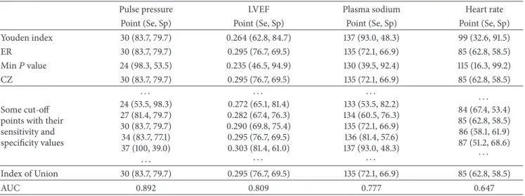
In this study, the data obtained from the study by Yildiran et al. [12] is used and all the methods including the IU method are applied to this data. The corresponding results are given in Table 9. The upper part of Table 9 shows the cut-points obtained by using the previously proposed methods. To define the cut-point with the IU method, some of cut-points with their sensitivity and specificity values and AUC value are given. According to this table, the IU method

(12)

ROC curve AUC = 0.809 0,0 0,2 0,4 0,6 0,8 1,0 Se ns itiv ity 0,2 0,0 0,4 0,6 0,8 1,0 1 − specificity x = 1 − Sp(cIU) = 0.305 x = 1 − AUC = 0.191 y = Se(cIU) = 0.767 y = AUC = 0.809

(a) The receiver operator characteristic curve for LVEF in the prediction of cardiovascular death [12] ROC curve AUC = 0.777 0,2 0,4 0,6 0,8 1,0 0,0 1 − specificity 0,0 0,2 0,4 0,6 0,8 1,0 Se ns itiv ity x = 1 − Sp(cIU) = 0.331 x = 1 − AUC = 0.223 y = Se(cIU) = 0.721 y = AUC = 0.777

(b) The receiver operator characteristic curve for plasma sodium in the prediction of cardiovascular death [12]

ROC curve AUC = 0.647 0,0 0,2 0,4 0,6 0,8 1,0 Se ns itiv ity 0,2 0,4 0,6 0,8 1,0 0,0 1 − specificity x = 1 − Sp(cIU) = 0.415 x = 1 − AUC = 0.353 y = Se(cIU) = 0.628 y = AUC = 0.647

(c) The receiver operator characteristic curve for heart rate in the prediction of cardiovascular death [12]

Figure 3: The receiver operator characteristic curves for LVEF, plasma sodium, and heart rate in the prediction of cardiovascular death [12].

gives the same cut-points with the ER method for different AUC values (Figure 3).

5. Conclusions

Defining the optimal cut-point is very important when a continuous variable is considered as a diagnostic marker. Getting optimal classification level depends on the point chosen for diagnosis. The criteria for optimality can change

according to the aim of the study. However, as a general rule, minimizing the total misclassification rates is a good approach. With IU method, since the difference between sensitivity and specificity values is minimum, this condition is met most of the time.

According to the results given in the tables, the proposed IU method can be a better alternative for defining the cut-point. When the definition of optimal point is stated as the point that minimizes the misclassification rates or the point

(13)

that equalizes the values of sensitivity and specificity, the IU method is better than the other methods in most of the comparison scenarios. This conclusion does not change with the distribution of biomarker or the homogeneity of variances of biomarkers. The changes in the sample size and the AUC values may affect but not alter the interpreta-tion.

The IU method uses the absolute difference between diagnostic accuracy measures and AUC value instead of using the Euclidean distance. The reason behind this idea is to provide the simplicity in defining the point as optimal. With the IU method, one can easily identify the optimal cut-point only by checking whether the sensitivity and specificity values are close enough to AUC value or not. That is, the complex calculations are not necessary for the IU method.

When the relative bias and MSE values of the IU method are compared with the previous methods, it is seen that the IU method is better than the others. Thus this method can be used for defining the optimal cut-point value especially when the sample sizes of the two groups are equal and the AUC value is high. (i.e., higher than 0.7).

A common practice is to select a cut-point which defines two risk groups for a continuously measured biomarker [16]. A cut-point for a biomarker is meaningful for the clinicians when it is clinically interpretable and understand-able. Clinical meaning for a cut-point can be explained by using its accuracy, that is, true classification rate. Among all the methods, only two of them, the Youden index and the concordance probability, are based on the maximization of this rate. Thus, these methods provide interpretable cut-points.

The point closest to(0, 1) point on the ROC curve method

involves a quadratic term and clinical meaning of this term is unknown. Despite the lack of clinical meaning, it is shown in the literature that this method is superior to the other methods in estimating the true cut-point [11].

The IU method, like the Youden index and the concor-dance probability, tries to minimize the misclassification rate. Hence, it also provides an interpretable cut-point. In this study, it is shown that the IU method performs better than

(or equal to) the point closest to(0, 1) point on the ROC curve

method. Therefore, the use of the IU method is advised to get more interpretable and better optimized cut-point.

The IU method provides a cut-point whose sensitivity and specificity are equally high. This means that, in a cut-point determination process, if sensitivity and specificity are valued equally, the IU method seems to be the best option among all other methods.

Appendix

Identification of the True Theoretical

Cut-Point for the IU Method under

the Normal Homoscedastic Distribution Case

Let us consider the normal homoscedastic distribution

sce-nario, where𝑋_𝐷∼ 𝑁 (𝜇_𝐷, 𝜎_𝐷), 𝐷 = 0, 1 (assuming 𝜇₁> 𝜇₀=

0 and 𝜎0 = 𝜎1 = 1). Then, the conditional distribution of the

quantitative variable𝑋 in group 𝐷 is 𝐹_𝐷(𝑐) = 𝑃(𝑋 ≤ 𝑐 | 𝐷)

for𝐷 = 0, 1.

In particular, at cut-point 𝑐, specificity Sp(𝑐) = 𝐹₀(𝑐),

and sensitivity Se(𝑐) = 1 − 𝐹₁(𝑐). Then the IU function can

be written as one of the following forms (according to the difference in the absolute value):

(i) IU(𝑐) = 𝐹₀(𝑐) − 𝐹₁(𝑐) + 1 − 2 ∗ AUC

(ii) IU(𝑐) = 1 − 𝐹₀(𝑐) − 𝐹₁(𝑐)

(iii) IU(𝑐) = 𝐹₀(𝑐) + 𝐹₁(𝑐) − 1

(iv) IU(𝑐) = 2 ∗ AUC − 1 − 𝐹₀(𝑐) + 𝐹₁(𝑐)

That is, IU(𝑐) = 𝛼𝐹₀(𝑐) + 𝛽𝐹₁(𝑐) + 𝛾 where 𝛼, 𝛽 and 𝛾 are

arbitrary(𝛼, 𝛽 = −1 or 1, −1 ≤ 𝛾 ≤ 1). Thus this formulation

is general form of the Youden Index. So, the cut-point which optimizes the IU function can be obtained by taking the

first derivative of IU(𝑐), 𝜕IU(𝑐)/𝜕𝑐 = 𝛼𝑓₀(𝑐) + 𝛽𝑓₁(𝑐), where

𝑓_𝐷(𝑐) = 𝜕𝐹_𝐷(𝑐)/𝜕𝑐 are the normal probability density

func-tions for diseased and nondiseased subjects. Since the normal

distribution is symmetric,𝑓₀ = −𝑓₀for the standard normal

distribution and thus the root of𝜕IU(𝑐)/𝜕𝑐 = 0 is 𝑐_IU= 𝜇₁/2.

Conflicts of Interest

The author declares that there are no conflicts of interest regarding the publication of this paper.

Acknowledgments

The author gratefully thanks Dr. Refik Burgut, Dr. Nazan Alparslan, and Dr. Yasar Sertdemir for their valuable com-ments and suggestions and also thanks Dr. Tansel Yildiran for providing the data to illustrate the method.

References

[1] X.-H. Zhou, N. A. Obuchowski, and D. K. McClish, Statistical Methods in Diagnostic Medicine, Wiley Series in Probability and Statistics, Wiley-Interscience [John Wiley & Sons], New York, 2002.

[2] M. H. Zweig and G. Campbell, “Receiver-operating charac-teristic (ROC) plots: a fundamental evaluation tool in clinical medicine,” Clinical Chemistry, vol. 39, no. 4, pp. 561–577, 1993. [3] M. S. Pepe, The Statistical Evaluation of Medical Tests for

Classification and Prediction, vol. 28 of Oxford Statistical Science Series, Oxford University Press, Oxford, UK, 2003.

[4] N. J. Perkins and E. F. Schisterman, “The inconsistency of “optimal” cut-points using two ROC based criteria,” American Journal of Epidemiology, vol. 163, no. 7, pp. 670–675, 2006. [5] W. J. Youden, “Index for rating diagnostic tests,” Cancer, vol. 3,

no. 1, pp. 32–35, 1950.

[6] R. Fluss, D. Faraggi, and B. Reiser, “Estimation of the Youden index and its associated cutoff point,” Biometrical Journal, vol. 47, no. 4, pp. 458–472, 2005.

[7] N. J. Perkins and E. F. Schisterman, “The Youden index and the optimal cut-point corrected for measurement error,” Biometri-cal Journal, vol. 47, no. 4, pp. 428–441, 2005.

[8] R. Miller and D. Siegmund, “Maximally selected chi square statistics,” Biometrics. Journal of the Biometric Society, vol. 38, no. 4, pp. 1011–1016, 1982.

(14)

[9] X. Liu, “Classification accuracy and cut point selection,” Statis-tics in Medicine, vol. 31, no. 23, pp. 2676–2686, 2012.

[10] K. H. Zou, C.-R. Yu, K. Liu, M. O. Carlsson, and J. Cabrera, “Optimal thresholds by maximizing or minimizing various metrics via ROC-type analysis,” Academic Radiology, vol. 20, no. 7, pp. 807–815, 2013.

[11] M. Rota and L. Antolini, “Finding the optimal cut-point for Gaussian and GAMma distributed biomarkers,” Computational Statistics & Data Analysis, vol. 69, pp. 1–14, 2014.

[12] T. Yildiran, M. Koc, A. Bozkurt, D. Y. Sahin, I. Unal, and E. Acarturk, “Low pulse pressure as a predictor of death in patients with mild to advanced heart failure,” Texas Heart Institute Journal, vol. 37, no. 3, pp. 284–290, 2010.

[13] E. F. Schisterman, N. J. Perkins, A. Liu, and H. Bondell, “Opti-mal cut-point and its corresponding Youden index to discrim-inate individuals using pooled blood samples,” Epidemiology, vol. 16, no. 1, pp. 73–81, 2005.

[14] J. Carpenter and J. Bithell, “Bootstrap confidence intervals: When, which, what? a practical guide for medical statisticians,” Statistics in Medicine, vol. 19, no. 9, pp. 1141–1164, 2000. [15] X. Robin, N. Turck, A. Hainard et al., “pROC: an open-source

package for R and S+ to analyze and compare ROC curves,” BMC Bioinformatics, vol. 12, article 77, 2011.

[16] D. Faraggi and R. Simon, “A simulation study of cross-validation for selecting an optimal cutpoint in univariate survival analysis,” Statistics in Medicine, vol. 15, no. 20, pp. 2203–2213, 1996.

(15)

Submit your manuscripts at

https://www.hindawi.com

Stem Cells

International

Hindawi Publishing Corporation

http://www.hindawi.com Volume 2014

INFLAMMATION

Behavioural

Neurology

Endocrinology

International Journal of

http://www.hindawi.com Volume 2014 Hindawi Publishing Corporation

Disease Markers

BioMed

Research International

Oncology

Journal of

http://www.hindawi.com Volume 2014 Oxidative Medicine and Cellular Longevity Hindawi Publishing Corporation

PPAR Research

The Scientific

World Journal

Immunology Research

Journal of

Obesity

Journal of

http://www.hindawi.com Volume 2014 Computational and Mathematical Methods in Medicine

Ophthalmology

Journal of

Diabetes Research

Journal of

http://www.hindawi.com Volume 2014 Research and Treatment

AIDS

Gastroenterology Research and Practice

Parkinson’s

Disease

Evidence-Based Complementary and Alternative Medicine Volume 2014 Hindawi Publishing Corporation