İSTANBUL BİLGİ UNIVERSITY
GRADUATE SCHOOL OF SOCIAL SCIENCES
FINANCIAL ECONOMICS GRADUATE PROGRAM
A QUANTITATIVE ANALYSIS ON STRESS TESTING APPLIED IN
CCPs: COMPARISON BETWEEN HISTORICAL SIMULATION
AND EXTREME VALUE THEORY
MASTER THESIS
FİLİZ ERTÜRK
TABLE OF CONTENTS
INTRODUCTION ... 1
1. CENTRAL COUNTERPARTIES AND THEIR RISK MANAGEMENT MECHANISMS ... 5
1.1.CENTRAL COUNTERPARTIES ... 5
1.2.CCP DEFAULT MANAGEMENT WATERFALL ... 8
1.2.1.Initial Margin of the Defaulted Member ... 8
1.2.2.Funded Guarantee Fund Contribution by the Defaulted Member ... 8
1.2.3.Dedicated capital of Clearinghouse for covered risks ... 9
1.2.4.Funded Guarantee Fund Contributions of Non-Defaulted Members ... 9
1.2.5.Additional Guarantee Fund Contributions of Non-Defaulted Members .. 10
1.2.6.Commitment from Remaining Capital of Clearinghouse ... 10
1.3.STRESS TESTING FOR CENTRAL COUNTERPARTIES ... 11
2. LITERATURE REVIEW ... 13
3. DATA AND METHODOLOGY ... 18
3.1.DATA ... 18
3.2.METHODOLOGY ... 19
3.2.1.Historical Simulation (HS) ... 20
3.2.2.Extreme Value Theory (EVT) ... 23
3.2.3.The Standard Portfolio Analysis of Risk (SPAN Algorithm) ... 30
4. RESULTS ... 34
4.1.RISK PARAMETERS DETERMINED via HISTORICAL SIMULATION ... 34
4.2.RISK PARAMETERS DETERMINED via EXTREME VALUE THEORY .. 35
4.2.1.Preliminary Data Analysis ... 35
4.2.2.Determination of the Threshold Values ... 36
4.2.3.Parameters and Tail Estimation ... 37
4.2.4.Risk Parameters under EVT ... 38
CONCLUSION ... 42 REFERENCES ... 45 APPENDIX ... 52
ABBREVIATIONS BIS Banks for International Settlements
BRSA Banking Regulation and Supervision Agency CCP Central Counterparty
CMB Capital Markets Board of Turkey
CPMI-IOSCO Committee on Payment and Market Infrastructures- International Organization of Securities Commission
EACH European Association of CCP Clearing Houses EMIR European Market Infrastructure Regulation
EVT Extreme Value Theory
GPD Generalized Pareto distribution
HS Historical Simulation
MEF Mean Excess Function
MLM Maximum Likelihood Estimation
OTC Over-the-Counter
PFMI Principles for Financial Market Infrastructures
POT Peaks over Threshold
PSR Price Scan Range
SCAP Supervisory Capital Assessment Program SPAN Standard Portfolio Analysis of Risk SSS Securities Settlement System
LIST of FIGURES
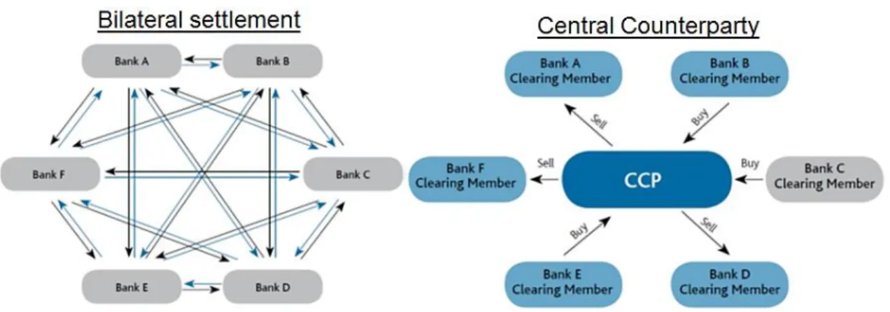
Figure 1- Bilateral Clearing and Central Clearing ... 5
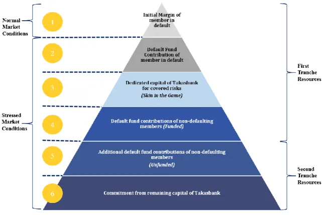
Figure 2- CCP Default Management Resources and the Order of Use... 7
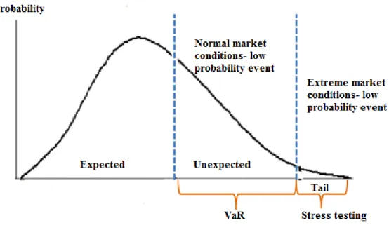
Figure 3- Value at Risk and Stress Testing on Probability Density Function ... 19
Figure 4- Block of Maxima vs. Peaks-over-threshold ... 25
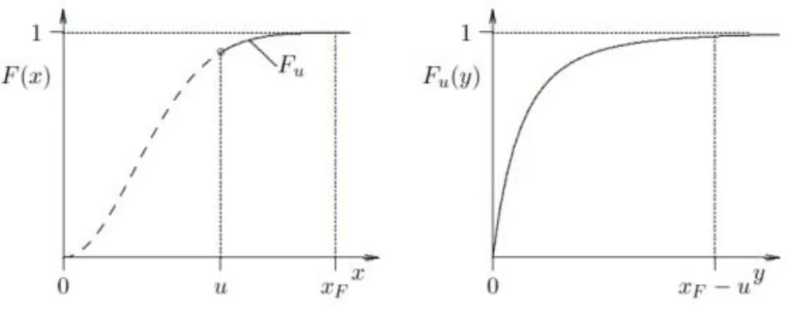
Figure 5- Distribution function of the data above threshold (u) ... 26
Figure 6- Comparative Results for Stress Testing ... 41
Figure 7- Q-Q Plots for the selected underlying in Borsa Istanbul Futures and Options Market ... 52
Figure 8- Descriptive Statistics for the selected underlying in Borsa Istanbul Futures and Options Market ... 55
Figure 9- MEF Graphs for the selected underlying in Borsa Istanbul Futures and Options Market ... 57
LIST of TABLES
Table 1- Scenarios used in determining Scanning Risk in SPAN ... 32 Table 2- Risk Parameters calculated via Historical Simulation ... 35 Table 3- Risk Parameters calculated via Extreme Value Theorem ... 39 Table 4- Shape and Scale Parameters for the selected underlying at different threshold levels and the percentage of the remaining part within the total distribution except from tail ... 60
ABSTRACT
The aim of this study is to apply and compare Historical Simulation (HS) and Extreme Value Theory (EVT) for stress testing that Central Counterparties (CCP), an important component for Securities Settlement Systems (SSSs), are obliged to implement according to the international regulations. In this regard, stress testing is conducted by constructing three days hypothetic portfolios which reflect the market concentration in the Borsa Istanbul Futures and Options Market where Takasbank submits CCP services. For both models, the risk parameters calculated for each underlying are used as input in the SPAN algorithm, which is the margining model used in this market, and the margin requirement under extreme market conditions are determined. The margin requirement arises from the potential default of the biggest two members with the highest exposure is compared with the existing default management resources. Results show that EVT produces higher levels of margin requirements since it models solely the rare events accumulated within the tails and that the resource requirement under stressed market conditions can only be covered for one day. On the other hand, the same default management resources are concluded to be sufficient to compensate the resource requirement calculated via HS for all three days.
ÖZET
Bu çalışmanın amacı, Menkul Kıymet Mutabakat Sistemleri’nin (SSSs) önemli bir öğesi olan Merkezi Karşı Taraf Kuruluşları’nın uluslararası düzenlemeler gereği uygulamak zorunda oldukları periyodik stres testlerinin Tarihsel Simülasyon (TS) metodolojisi ve Uç Değer Teorisi (UDT) ile tatbik edilmesi ve kıyaslamasının yapılmasıdır. Bu kapsamda, Takasbank’ın MKT hizmeti verdiği Borsa İstanbul Vadeli İşlemler ve Opsiyon Piyasası’nda (VİOP) piyasa konsantrasyonunu yansıtan üç günü temsil eden hipotetik portföyler için stres testi çalışması uygulanmıştır. Her iki model için dayanak varlık bazında hesaplanan risk parametreleri piyasadaki teminatlandırma metodolojisi olan SPAN’de girdi olarak kullanılmış ve uç piyasa koşulları altında üye bazında teminat gereksinimleri hesaplanmıştır. Bu koşullar altında en büyük iki üyenin temerrüdü halinde oluşacak toplam teminat gereksiniminin mevcut temerrüt yönetim kaynakları ile karşılanma seviyeleri analiz edilmiştir. Sonuçlar, sadece kuyruk kısmında biriken aşırı olayları modelleyen UDT ile daha yüksek teminat gereksinimlerinin elde edildiğini ve oluşturulan hipotetik portföyler için stres koşulları altında ihtiyaç duyulan kaynak gereksiniminin sadece bir gün karşılanabildiğini göstermiştir. Buna karşılık, aynı temerrüt yönetim kaynaklarının Tarihsel Simülasyon ile belirlenen stres testi parametrelerinin tatbik edilmesiyle oluşan kaynak ihtiyacını ise her üç gün için de rahatlıkla karşıladığı sonucuna ulaşılmıştır.
INTRODUCTION
The 2008 global financial crisis has clearly shown that Central Counterparty Institutions (CCPs) play a very significant role in enhancing the financial stability in today’s global markets. Thanks to their presence, risks are managed better and losses are minimized in buying-selling transactions. The insolvency of Lehman Brothers set an important example in this regard. When Lehman Brothers went bankrupt, the companies which have been counterparties in bilateral transactions suffered huge losses in case settlement has not taken place via CCPs or transactions held through OTC markets. On the other hand, the derivatives positions for which the settlement was done through LCH.Clearnet (CCP) were successfully finalized. Thus, potential counterparty losses were eliminated by the effective risk control mechanism of the clearing house (Cheah et al., 2012). Moreover, the crisis has disclosed the gaps within the banks’ risk management mechanisms as well. Accordingly, Banks for International Settlements (BIS) released Basel III standards in December, 2010 in order to enhance the regulation, supervision and risk management within the banking sector (Basel Committee on Banking Supervision, 2011). The main objective of this accord is to encourage banks to use CCPs for settlement of derivatives instruments and hence to mitigate the risks induced by trading environment.
Putting the Basel accords into force, regulatory bodies have extended the requirements for prudent risk management by covering all financial market infrastructures. Moreover, in April 2012, CPMI-IOSCO (Committee on Payment and Market Infrastructures- International Organization of Securities Commission), the
international standard-setting body in policy development and implementation for clearing, settlement and reporting arrangements, published the standards report Principles for Financial Market Infrastructures (PFMI) which set out new international standards for payment, clearing and settlement systems, including central counterparties. In this framework, banks have been allowed to use lower risk weight in their trade exposures to a Qualified CCP whereby the CCP is declared to be consistent with CPMI-IOSCO principles by the relevant competent authority. One of the requirements in these principles is that CCPs should have sufficient financial resources for the potential losses they may be exposed under normal and extreme market conditions. In technical terms, CCPs are expected to have sufficient size of guarantee fund to cover financial losses under extreme but plausible market conditions (CPMI-IOSCO, 2012). Moreover, CCPs should test the adequacy of their financial resources under extreme market conditions in case of the default of two clearing members with the highest exposure through stress tests to be applied at regular intervals (CPMI-IOSCO, 2012).
The need for stress testing and its significance for risk management by CCPs has been well presented in international regulations yet there is not a commonly-held approach regarding the methodology to undertake such tests. Different studies held by huge financial banks which focus on various markets have provided different conclusions about methodologies applied depending on the market and instruments analyzed and the time period used in those studies.
Even though there has been no worldwide standard method for the application of stress testing by CCPs, CPMI-IOSCO has defined, as criteria, the minimum confidence level of 99% to be used in calculating initial margin amounts in its PFMI, April 2012.
Moreover, within EMIR (European Market Infrastructures Regulation) framework, CCPs are obliged to use confidence level of 99% for cash equities and derivatives trading at organized markets; whereas, the level of 99.5% shall be used for OTC derivatives in respect of initial margins (EMIR EU 153/2013).
The aim of this study is to provide a comparison in determination of the market risk parameters in terms of price change which will be used in stress testing between Historical Simulation (HS) and Extreme Value Theory (EVT) and to conduct a quantitative analysis in respect of stress testing. In this regard, representing the market concentration, three-day hypothetical portfolios for Borsa Istanbul Derivatives Market, for which central counterparty service has been provided by Takasbank since March, 2014, have been constructed and risk parameters are calculated by applying Historical Simulation and Extreme Value Theory, separately. Moreover, stress testing has been applied by using these parameters in order to analyze the levels of compensation for potential losses by Takasbank’s default management resources under extreme market movements.
The results show that Extreme Value Theory, as a more conservative approach, produces higher levels of margin requirements since it models only the rare events accumulated within the tails and that the resource requirement under stressed market conditions can only be covered for one day. On the other hand, the same default management resources are concluded to be sufficient to compensate the resource requirement calculated via Historical Simulation for all three days. Besides, while Historical Simulation is easy to apply and explain, Extreme Value Theory requires a well-background of econometrics and takes more time to apply. Moreover, Extreme
Value Theory is open to variance-bias tradeoff since there is no automated algorithm to reach the optimal threshold level; hence different users can reach different loss results and the model may suggest misleading results in comparing the different periods or institutions.
Comparison of two different methods, namely Historical Simulation (HS) and Extreme Value Theory (EVT) is an important contribution to the literature in two points. One is that this is the first literature in Turkey which focuses on the stress testing methodology and examines the sufficiency of default fund size mandatorily applied by Central Counterparties. Secondly, except from Turkey, there are very few literatures worldwide analyzing the methodology of stress testing in CCPs and there has been no widely accepted model to use. Therefore, this study provides valuable information with regards to the hot debating issue of choice on stress testing methodology by analyzing real-like data for all of the underlying in such highly liquid and relatively volatile market environment.
The rest of the study is designed as follows: Section 1 describes the structure of CCPs and their role in the financial system as well as the associated risk management functionalities. Then Section 2 presents the obvious and most-cited literature related to Historical Simulation and Extreme Value Theory and their recent use in CCP stress testing as well. Afterwards, Section 3 gives details about the data and the methodology applied in the quantitative design of this study. Lastly, Section 4 presents the risk parameters for each underlying calculated via each model and corresponding stress testing results.
1. CENTRAL COUNTERPARTIES AND THEIR RISK MANAGEMENT MECHANISMS
1.1. CENTRAL COUNTERPARTIES
As an important component of Securities Settlement Systems (SSSs), a Central Counterparty (CCP) undertakes the settlement finality by interposing itself between counterparties to contracts and becomes the buyer to every seller and the seller to every buyer (Bank for International Settlements, 2004). By this functionality, CCPs carry out a standardized risk management mechanism by centralizing the risks that the parties have against each other, reduce the systemic risks that market participants may be exposed to and thus contribute to achieving financial stability. The display of central counterparty service in term of market regulation is presented at Figure 1 as below.
Source: Moscow Exchange, Available at http://fs.rts.ru/files/5640.
In Turkey, Takasbank has authorized to offer central counterparty services for the exchange traded financial instruments by using the legal basis that the new Capital Markets Law No. 6362 entered into force on 30.12.2012 has provided. Takasbank first began to submit this service as of September 2, 2013 in the Securities Lending Market operated under its roof, and as of March 3, 2014, in the Borsa Istanbul Futures and Options Market, and as of October 7, 2016 in the Borsa Istanbul Money Market. Moreover, Takasbank has been declared as Qualified CCP on 23.03.2016 by Capital Markets Board (CMB) as the competent authority in Turkey, by which the transactions that the Turkish banks have through Takasbank CCP serviced markets have been considered as “qualified transactions” and those banks have the low risk weight advantages in their risk exposures to be recorded in the solo or consolidated capital requirement calculations1.
The international regulations suggest the CCPs to construct a multilayered defense mechanism in order to carry out their unique functionality (CPMI-IOSCO, 2012; EMIR (EU) 153/2013). This defense mechanism includes firstly defining effective criteria for entry to/withdrawal from the membership. Secondly, establishing a default management waterfall including margins to be used in case of any member default, funded guarantee fund contributions collected from members, unfunded guarantee fund contributions that the members commit and the allocated and committed capital amounts from the capital that the CCP assessed (Lazarow, 2011). Moreover, this layer also covers determination of the assets to be accepted as collateral and the basis for valuation of them. Finally, default management process to follow in case of any default of member
1
and the actions to take should be clearly defined in the relevant market rules and procedures.
The financial resources and the order of use that CCPs use in case of any default have been stated in the international regulations and also presented in Figure 2 below in specific to Takasbank which has the authority to submit central counterparty services in Turkey for the specified markets in regulations.
Source: Takasbank, Available at: Takasbank Disclosure Framework, April 2016
1.2. CCP DEFAULT MANAGEMENT WATERFALL
1.2.1. Initial Margin of the Defaulted Member
As the first line of defense, initial margin is requested when the member wants to take positions in order to cover the potential future exposures to a participant (EMIR EU 153/2013). CPMI-IOSCO and EMIR set a minimum of 99% confidence interval and one year look back period with two day holding period in calculating the initial margins for the exchange traded financial instruments (CPMI-IOSCO, EMIR EU 153/2013). Takasbank applies these rates as 99.5% confidence interval, 1250 days look-back period and two day holding period in initial margin calculations.
1.2.2. Funded Guarantee Fund Contribution by the Defaulted Member According to the 42nd Article of EMIR (EU) No. 648/2012, the size of guarantee fund should be determined with 99.9% confidence level with a size at least the maximum resource requirement arises due to the default of the biggest member having the largest exposure or to the concurrent default of the second and third biggest members having the largest exposure. The size of guarantee fund is allocated within the market members according to their exposures.
Determining this resource requirement, Takasbank takes the uncovered risk levels that cannot be compensated by the initial margins. The uncovered risk is qualified as the difference between the margin requirement calculated with 99.9% confidence interval and two day holding period and the initial margin amounts.
1.2.3. Dedicated capital of Clearinghouse for covered risks
In case of any default, the losses exceed the initial margin and guarantee fund contribution amounts of the defaulted members have been compensated by the dedicated capital of Clearinghouse for covered risks without reflecting the loss to non-defaulted market participants. This amount is declared publicly for each market that CCP service is provided by specifying the period in which it will be valid via the corporate website of the Clearinghouse.
Determining the dedicated capital amount, Takasbank takes account the Basel II capital adequacy arrangements, EMIR Master Document (EU) No 648/2012 of the European Union, EMIR technical arrangement (EU) 152/2013 and (EU) 153/2013 on the capital adequacy and default waterfall of the central counterparty institutions. In this regard, the capital assessed by Takasbank for covered risk should be at minimum 25% of the amount which is found by adding the 75% of the previous year’s operational expenses related to the CCP services for general business risk and recovery and orderly wind-down to the minimum capital amount calculated within the framework of the banking regulation for risks subject to the legal capital adequacy. This amount is allocated among the markets for which central counterparty services are provided according to the decision that Takasbank Board of Directors has taken.
1.2.4. Funded Guarantee Fund Contributions of Non-Defaulted Members This defense line indicates the guarantee fund contribution amount of non-defaulted members which is allocated by taking into consideration the exposures that
they possess. In case that the assessed capital has become insufficient to cover losses, funded Guarantee Fund contributions of non-defaulted members have been utilized.
1.2.5. Additional Guarantee Fund Contributions of Non-Defaulted Members
The Article No 43 of EMIR (EU) 648/2012 states that CCPs have the authority to demand additional guarantee fund contributions in case of any default of market participants if needed. Pursuant to Takasbank CCP Regulation, additional guarantee fund can be requested from the participants at most four times in one year as not exceeding the funded guarantee fund contribution amount that the members deposited for the relevant month.
1.2.6. Commitment from Remaining Capital of Clearinghouse
As the latest line of defense, calculation of committed capital amount by Takasbank is applied in accordance with the regulations that are Basel II capital adequacy arrangements, EMIR Master Document (EU) No 648/2012 of the European Union, EMIR technical arrangement (EU) 152/2013 and (EU) 153/2013 on the capital adequacy and default waterfall of the central counterparty institutions. In this regard, commitment made from the remaining capital of Takasbank is calculated by subtracting the dedicated capital for covered risks and the minimum capital requirement set by Banking Regulation and Supervision Agency (BRSA) from the equity capital calculated based on the Regulation on Equity of Banks2 by BRSA.
2
This amount is declared publicly for each market that CCP service is provided by specifying the period in which it will be valid via the corporate website of the Clearinghouse.
1.3. STRESS TESTING FOR CENTRAL COUNTERPARTIES
An efficient financial resource management is crucial for CCPs to prevent the contagion risk of counterparty default in protecting both their members and themselves from losses (Duffie and Zhu, 2011). In case of any default under extreme but plausible market conditions, CCPs try to prevent the reflection of losses on non-defaulted members by activating its dedicated capital for covered risks after utilizing the initial margins and guarantee fund contribution of the defaulted member. If the loss cannot be covered with the allocated capital of CCP, the funded guarantee fund contributions and unfunded guarantee fund commitments provided by non-defaulted members have been activated. As the last resort, the commitment made from the remaining capital by the Clearinghouse has been utilized to solve the default.
The functioning mechanism of the default management waterfall highlights the question at which level the resource requirement will be adequate in case of any possible default of market participants. Because the possible loss can leap to other participant if the initial margin and guarantee fund contribution amounts have been underestimated; on the other hand, by overestimating the margin levels cause the cash and assets in collateral accounts to be idle which in the end leads renouncing from profit and growth as well (Cumming and Noss, 2013). For this reason, CPMI-IOSCO, the international authority to enhance coordination of standard and policy development and implementation arrangements, has forced the CCPs to implement regular stress testing
application in order to analyze the sufficiency of its default management resources against the extreme but plausible situations by its publication of the core principles published on April 2012 . Moreover, as the body of European legislation for over-the-counter (OTC) derivatives, central over-the-counterparties and trade repositories, EMIR adopts a technical risk management structure in its (EU) No. 153/2013 and the Article 53 of this regulation makes it mandatory for CCPs to analyze the sufficiency of their financial resources against the concurrent default of the biggest members under stressed market conditions (EMIR (EU) 153/2013).
In this regard, stress testing implementation highlights the strategic planning of CCPs in determining the allocated and committed capital amounts and the level of reflection of the possible losses in case of any default to the non-defaulted members (Elliott, 2013).
2. LITERATURE REVIEW
Stress testing firstly began in the 1980s as a risk management tool to analyze mainly the interest rate risk (Kapinos et al., 2015). After declaration made by Basel Committee on Banking and Supervision, at December 1995, that VaR method would be used in calculation of the capital adequacy of banks and that many large financial institutions are required to implement stress testing for liquidity and market risks in their trading books, stress testing has become a widely used application in assessing market, liquidity and occasionally credit risk by banks and large financial institutions (Fender, Gibson and Moser, 2001). Moreover, since Basel II Accord directly links the stress testing and risk capital, the practitioners have involved re-examination of stress testing methodologies (Rowe, 2005).
More recently, after the 2008 financial crisis, the stress testing in macroeconomic perspective conducted within the framework of the Federal Reserve’s Supervisory Capital Assessment Program (SCAP) has perceived as successful due to its focus on the estimation of the scale of recapitalization needed by the financial sector (Kapinos et al., 2015). Additionally, in 2009, the Committee of European Banking Supervisors (CEBS) conducts EU-wide stress testing with 22 cross-border banks and in 2011 the sample has extended with 90 largest banks.
Since Central Counterparties are both financial institutions and an element of Securities Settlement Systems, they engage with stress testing in both terms. Besides, some CCPs have the banking license like Takasbank and LCH.Clearnet, they also take attention into stress testing since they are binding with different regulations. In April 2012, CPMI-IOSCO sets out new international standards covering CCPs that they
should test the adequacy of their financial resources under extreme market conditions in case of the default of two clearing members with the highest exposure through stress tests to be applied at regular intervals (CPMI-IOSCO, 2012). Besides, EMIR adopts a technical risk management structure in its (EU) No. 153/2013 regulation that CCPs are obliged to analyze the sufficiency of their financial resources against the concurrent default of the biggest members in stressed market conditions (EMIR (EU) 153/2013). Furthermore, Lazarow (2011) conducts a survey with the central counterparties throughout the world on their current risk management mechanisms and concludes a common expectation that margin amount and funded guarantee fund contribution of the defaulted member would be enough in resolving the default. Moreover, the vast majority accepts the utilization of additional resources within the default management waterfall only in case of a concurrent default of few biggest members.
In stress testing applied by CCPs, the main aim is to analyze the sufficiency of existing resources against the resource requirement occurred in the extreme but plausible market conditions. Therefore, the attention is given to the extreme losses which are observed within the tails of distribution (Daouia, 2016). The analysis of tail behavior has great attention that there are numbers of studies which focus on the fat tail behavior of financial return values. Longin (1996), Longin (1997a, b), Danielsson and de Vries (1997), Klüpelberg et al. (1998), Mcneil (1998) and Huisman et al. (1998) present the fat tail behavior by analyzing stock returns; on the other hand, Zangari (1996a), Huisman et al. (1997) and Venkataraman (1997) provide studies on the fat tail behavior of exchange rate returns. Moreover, Longerstaey et al. (1996) and Lucas (1997) focus on all markets.
Value at Risk approach has been widely used in risk management industry until recent period as the methodology in stress testing (Benselah, 2000). Started to be used in examining market risk during 1980s, this approach has become a standard method of measurement with the launch of “RiskMetrics” by JP Morgan at 1995 (Lourens, 2013).
According to Perignon and Smith (2006) survey, 73% of banks among 60 US, Canadian and large international banks over 1996-2005 have reported that the VaR methodology used by those banks was based on Historical Simulation. Li et al. (2012) state that Historical Simulation is a good resampling model due to its simplicity and lack of distributional assumption. Brooks and Persand (2000) analyze the Historical Simulation in terms of data sample adequacy. They suggest that too short data set introduces the risk of ignoring past stresses, whereas using only very recent data set enables the model to reflect current market dynamics better. Dominguez and Alfonso (2004) develop an empirical stress testing by applying Historical Simulation and Monte Carlo Simulation to measure the potential loss under two historical event scenarios. They conclude that the response of VaR methodologies to stress testing is different from each other that Monte Carlo Simulation demonstrates more sensitivity.
After the 2008 financial crisis, the use and shortcomings of traditional VaR estimates have been questioned (Turner, 2009). Alexander and Sarabia (2012) examine the dependence of regulators on VaR models for capital adequacy calculations and their failure in the crisis. Another approach in calculating the tail losses is Extreme Value Theory (EVT) which only incudes the extreme events within the tail end of a distribution of returns into the model (Tsay, 2010). EVT is mostly used model in applied sciences such as engineering and insurance (Reiss and Thomas, 1997; McNeil, 1999).
Various research studies highlight the potential usage of EVT in financial risk management in analysis of currency crisis, stock market turmoil and credit defaults (Diebold et al., 1998). Singh et al. (2011) apply EVT to analyze extreme market risk for the Australian Index and the S&P 500 Index. They suggest that EVT can successfully reflect the Australian stock market return series for predicting daily VaR.
Longin (2000) implements an EVT approach in order to calculate the Extreme VaR for S&P 500 Index and states its three advantages over traditional VaR models that are the parametric nature enabling to calculate the high probability values, reducing model risk by not assuming any distribution for the sample data and covering only extreme events which produces more accurate forecast.
Klüperberg et al. (1998) compare the daily VaR results calculated with Historical Simulation, Extreme Value Theory and another method based on normality assumption for German DAX Index. They suggest that VaR calculated with the normality assumption gives underestimated results compared to other methods.
Gençay and Selçuk (2004) examine the daily stock market returns of nine different emerging markets by incorporating variance-covariance method, Historical Simulation and Extreme Value Theory and then conduct stress testing to analyze the tail forecasts of daily returns. Their findings suggest that EVT method dominates the other methods in terms of VaR forecasting.
There are few literatures focusing on the methodology used in CCP’s stress testing. As a hot-debated issue ongoing by international associations and regulators, there has been no standardized method in application of mandatory stress testing. European Association of CCP Clearing Houses (EACH), Takasbank is also one of its
members, publishes “Best practices for CCPs stress tests3” in April 2015 by which
EACH aims to summarize their findings and present recommendations to address some of the best practices. On their note, the focus is especially on principles to apply when CCPs perform stress testing such as relevance, structure, governance etc. and the areas that would be subject to best practices.
As one of the few academic researches, Lourens (2013) compares different measures to analyze extreme losses in the South African Equity derivatives Market in order to estimate the size of guarantee fund of Safcom, the CCP for exchange traded derivatives in South Africa. She applies Historical Simulation VaR, Conditional VaR, Extreme VaR and stress testing during historic periods of stress in the market. The study concludes that Extreme VaR predicts more accurate results in extreme losses and consequently in the guarantee fund size.
Another research made by Cumming and Noss (2013) proposes the application of EVT techniques in order to examine the distribution at the tail of returns in determination of the initial margin and default fund levels of CCPs from the perspective of the Bank of England.
As more recent study, Eriksson (2014) compares different models including Historical Simulation, EVT and copula models to estimate the risk of a portfolio by applying joint distribution of asset. He concludes that Historical Simulation is completely non-parametric to handle the dependence which underestimates the risk in stress testing applications. On the other hand, he finds that although EVT models only the extreme events, it produces the largest sampling error and too much conservative.
3
3. DATA AND METHODOLOGY 3.1. DATA
International regulations (CPMI-IOSCO, EMIR EU 153/2013) require the use of minimum one year data in calculating the risk parameters to be used in margining and stress testing; whereas, Takasbank uses the data of 1251 days in order to be more prudent. In this regard, three-day portfolios representing the concentration in the Borsa Istanbul Derivatives Market have been prepared and historical prices of underlying in the market have been obtained from Bloomberg and Reuters.
In calculating the risk parameters, MS Office Excel program and EVIM MATLAB package developed by Gençay et al. (2001) have been used for Historical Simulation and Extreme Value Theory, respectively. Moreover, EVIEWS has been run to analyze the descriptive statistics of daily return data.
Similarly, in consistent with international regulations, while 99.5% confidence level and two day holding period have been applied in risk parameter calculations for margining under normal market conditions, 99.9% confidence level and 3 day holding period have been used to reflect the extreme market conditions.
Following the risk parameter calculation, the portfolios representing the market concentration have been margined for both HS and EVT by applying the portfolio based SPAN algorithm which is the model used for margining in this market. The resource requirement occurs in case of the default of two members with the highest exposure has been compared with the default management resources explained in Section 1.2 and the level of coverage has been analyzed for both models.
3.2. METHODOLOGY
In application of stress testing, to what extent the uncovered risk amounts that CCPs may face under extreme but plausible market conditions can be covered with the existing financial resources has been measured. Taken into consideration the returns of the portfolios whose settlement is performed through CCPs, one should concentrate on tails where extreme profits/losses are observed (Daouia et al., 2016). Put it differently, in order to specify the magnitude of loss which is not expected to be observed in 99% of the time, but expected to be observed in 1%, the value at risk (VaR) is measured. Namely, margining is conducted by not taken into consideration the 99 days that normal market conditions are reflected, but the 1 remaining day. Figure 3 shows VaR and corresponding stress testing on a distribution by highlighting normal and extreme market conditions.
Determining the potential loss that may arise under extreme market conditions, this study concentrates on Historical Simulation Model which has been widely used by banks and other financial institutions and Extreme Value Theory which is relatively new in financial analysis in risk parameter calculation.
3.2.1. Historical Simulation (HS)
After the extreme events such as 1987 Wall Street Crisis, 1997 Asian Crisis and 2008 global financial crisis, investors and financial institutions have concentrated their attention on measuring the extreme market conditions. Value at Risk approach has been widely used in risk management industry until recent period (Benselah, 2000). Started to be used in examining market risk during 1980s, this approach has become a standard method of measurement with the launch of “RiskMetrics” by JP Morgan at 1995 (Lourens, 2013). Moreover, Basel Committee on Banking and Supervision, at December 1995, declared that VaR method would be used in calculation of the capital adequacy of banks4. Furthermore, U.S. Securities and Exchange Commission (SEC) released a proposal indicating that publicly held companies should disclose quantitative information about their derivatives activity by using one of the three VaR models (Jorion, 1996).
VaR figures out the maximum loss in the value of an asset or a portfolio predicted under normal market conditions over a specific time interval (n) at a given confidence level (α). Moreover, it can be explained to be the minimum loss under extreme market conditions over a specific time interval (n) at a given probability (1-α)
4
(Longuin, 1999). While the first approach concentrates on the center of the distribution, the latter models the tail. For example, assuming that the VaR for one day and at 95% confidence level is 100k TRY, it can be described that the value of this asset will decrease more than 100k TRY for the following day at 5% probability. In other words, one can be sure that there won’t be more than 100k TRY loss at 95% confidence level.
There are three approaches in calculating VaR value that are Parametric Method, Historical Simulation and Monte Carlo Simulation. This study incorporates Historical Simulation which is the most widely accepted (Mehta et al, 2012) and also used by Takasbank in risk modeling.
Value at Risk with Historical Simulation has been used to find the maximum loss that an asset or a portfolio may face in near future by taking their past performance into consideration with a specified holding period and confidence level (Linsmeier ve Pearson, 2000). Based on the assumption that history is repeating itself, daily returns are calculated by gathering the relevant data belonging to the past (Li et al., 2012). The historical price changes are used to simulate the possible movements in prices in the near future. Namely, using the K days historical data enables the simulation of possible K price changes from today to tomorrow (Dowd, 1998).
VaR with HS at confidence level of α can be expressed in mathematical terms as below:
By using the empirical distribution of past returns to generate VaR, Historical Simulation is a non-parametric approach which does not make any assumptions about the shape of the distribution (Pritsker, 2001). Therefore, it is an easy-to-understand and quickly applicable measurement tool which makes the model to be widely preferred (Asberg and Shahnazarian, 2008). Moreover, the widespread use of this model may be attributed to the fact that it is recommended by international regulators, especially BIS (Bank for International Settlement) and is applied by top level international financial institutions (Çifter et al., 2007). On the other hand, Historical Simulation has the limitation in its i.i.d. assumption of returns that it assigns the equal probability weight to each day’s return meaning that historically simulated returns are independently and identically distributed (i.i.d.) through time (Jorion, 1996; Christoffersen, 2006). However, it is known that the volatility of asset returns tends to change through time, and that periods of high and low volatility tend to cluster together (Bollerslev, 1986). Moreover, since the output is directly resulted from historical data, misleading results can be obtained in case of using data sample that does not reflect market changes (Linsmeier and Pearson, 2000). In addition, there are some studies showing that the HS may calculate the VaR amount lower than the actual value since there may not be enough data within the high quantiles (Benselah, 2000).
On the other hand, similar with HS in terms of not assuming a specific distribution, Extreme Value Theory (EVT) has become increasingly used in financial modeling by the virtue of its focus on extreme outcomes i.e. catastrophic events (Gilli and Këllezi, 2006).
3.2.2. Extreme Value Theory (EVT)
Traditional methods for financial risk measures adopt normal distributions as a pattern of the financial return behavior. Moreover, they fit models to all data even if the main focus is on extremes. On the other hand, there are many academic studies revealing that financial returns have fat tail distribution (Hols and de Vries, 1991; Longin, 1996; McNeil, 1998; Ghose and Kroner, 1995; Gençay et al., 2003; Dacorogna, Gençay et al., 2001). The fat tail characteristic of financial returns indicates that probability of extraordinary movements in prices is higher than what normal distribution predicts and it causes greater potential loss than a normal distribution (Coronado, 2001). Analyzing the financial risks driven by extreme events, the tail behavior of the probability distribution and estimating relevant probabilities of occurrence become a starting step (Hult et al., 2012). Moreover, at which speed probability density function approaches to zero while the loss amount, theoretically, approaches to infinity is crucial. That is how slow the speed of function to approach zero, distribution is qualified as fat tail due to the higher value of probabilities of corresponding values (Klugman et al., 1998).
In stress testing, the focus is on unexpected losses under extreme market conditions. Therefore, analyzing these losses more accurate, the tail behavior becomes crucial since the extreme gains and losses are accumulated in these areas (Daouia, 2016). Moreover, concentrating on the frequency and magnitude of extreme events rather than all events in the data set like Historical Simulation, the results would be more accurate in analyzing extreme market conditions (Coronado, 2001).
At that point, Extreme Value Theory (EVT), mainly used in analyzing the extreme events in climatology and hydrology (e.g. flood, earthquake, tsunami etc.),
comes into prominence in modeling the risk under extreme but plausible market conditions in finance (McNeil,1997; Embrechet et al., 1997; Reiss and Thomas, 1997; De Haan et al., 1994).
EVT is a powerful and fairly robust framework (Magnou, 2016) to analyze the tail probabilities of financial returns and to model their asymptotic behavior (Coles and Davison, 2008). This model focuses not on all observations but on the observations in the tail area where extraordinary events take place (Stoyanov et al., 2011).
There are two approaches in EVT to estimate the potential loss driven by extreme values representing extreme events within the data:
1. The block of maxima method 2. The peaks-over-threshold method
As a traditional approach, in the block of maxima method, data is divided into consecutive blocks of equal size and the focus is given to the series of maxima of the returns in these blocks (McNeil, 1999). The choice of the size of blocks (three months, six months, one year etc.) and the length of the time series become controversial issue since the decision has direct effect on results (Stoyanov et al., 2011).
On the other hand, as a more modern approach, in the peaks-over-threshold method, a value for the high threshold is chosen and the distribution constituted by the sample which exceeds the threshold is fitted to the Generalized Pareto Distribution (GDP) (Gilli and Këllezi, 2006). This model requires a very large sample in order to get sufficient number of observations from the tail as exceedance and a well selection of threshold value to correctly separate the body of distribution and the starting point of tail (Stoyanov et al., 2011).
Figure 4 shows a comparison of two approaches in graphical view where the left panel represents for the block of maxima method while the right panel is for the peaks-over-threshold method.
Source: Gilli and Këllezi, 2006.
Figure 4- Block of Maxima vs. Peaks-over-threshold
Removing the disadvantages in the first approach, this study is based on the peaks-over-threshold method as there is enough data, 1250 day financial returns, to obtain meaningful results since the suggested period is 1000 days (Goldberg et al., 2008).
3.2.2.1. The peaks-over-threshold method (POT)
Developed as an alternative model to the classical approaches by Smith (1989), Davison-Smith (1990) and Leadbetter (1991), the peaks-over-threshold method directly focuses on the tail area of distribution and provides estimation based on the exceedance over a selected high threshold which is fitted to GPD.
Source: Önalan, Ö. (2003).
Figure 5- Distribution function of the data above threshold (u)
As shown in the Figure 5 above, the distribution function is called the excess distribution function which represents the distribution of extreme values (x) over specified threshold (u) and is defined as:
where is a random variable, is a given threshold, are the excesses.
This function indicates the probability that, under the assumption that exceeds , x values can exceed at most .
According to this model for which the first steps taken by Balkema and de Han (1974) and Pickands (1975) and then developed by Davison-Smith (1984) and Castillo (1997), in case that a large threshold value is selected, the distribution function belonging to the exceedance can be fitted to GPD and as the threshold value gets larger enough, the distribution function converges to GPD (Mazilu, 2010). In other
words, while the threshold goes to the rightest point of the distribution, the distribution gets closer to the function expressing GPD which can be defined as:
for if ξ ≥ 0 and y ∈ [0, −β/ξ] if ξ < 0. Here is the shape parameter and is the scale parameter for GPD.
The value that the scale parameter takes determines the tail behavior of the distribution. According to this, if is greater than zero, the F distribution function represents a fat tail distribution; if is lower than zero, F represents thin tail distribution and if equals to zero, the distribution represents a normal distribution. Since the upper limit cannot be set for financial losses, the distributions where the shape parameter takes positive values would be appropriate to include into the model (Gilli and Kellezi, 2000).
The importance of the model by Balkema and de Han (1974) and Pickands (1975) is that GPD can be estimated in case that the shape and scale parameters with a high threshold value are determined (Gençay et al., 2001). To obtain this, while methods like Probability Weighted Moments, Bayesian models or maximum likelihood method can be applied, Hosking and Wallis (1987) provides evidences in their study that maximum likelihood method produces more accurate results.
3.2.2.2. Steps in Estimating Tail of the Distribution (Calculating Value at Risk)
1st step: A large threshold value is determined for the sample data.
Selection of the threshold value is very crucial because too high threshold value results in too few exceedance by which the meaningful data is excluded from the model that consequently gives high variance. On the other hand, too low threshold value generates biased estimators, so the expected loss becomes lower than the actual potential loss (Roth et al., 2015). Moreover, in order to make a real-like estimation, there should be enough data above the selected threshold as well as determining a high threshold value (Balkema and de Han (1974), Pickands (1975)). Assessing a correct threshold also provides information about where the tail starts (Benselah, 2000).
However, there has been no automated algorithm with a satisfactory performance for the selection of threshold value yet (Magnou, 2016). The threshold is typically chosen subjectively by looking at some plots like Pareto Quantile Plot, Hill Graph or Mean Excess Function (Embrechts et al., 1997).
As a widely used tool in risk, insurance and extreme values (Ghosh and Resnick, 2010), Mean Excess Function (MEF) is an empirical estimation which divides the sum of the values above threshold by the number of data points which exceeds the threshold value (Gençay et al., 2001). In determination of the threshold value, data points are analyzed whether they constitute a linear trend above different threshold value candidates. The threshold value as starting point of linear trend indicates that the values above selected threshold converges GPD with a positive shape value (McNeil, 1997a).
This function also gives information about the tail behavior of the distribution by analyzing the trend that data points follow. If the data over threshold follows a positive trend, the distribution is said to be fat tail; if the trend is negative, the distribution becomes thin tail; and if the trend is a horizontal line, the distribution is exponential distribution (Embrechts, 1997; Gençay et al., 2001).
2nd step: Shape and scale parameters are estimated via maximum likelihood model by applying the GDP for the values exceed threshold.
3rd step: The tail of distribution is defined for the values exceed threshold. Representing the distribution of the values above a high threshold, distribution function has been defined at Section 3.2.2.1 as below:
Since for , the equation becomes:
and replacing by the GPD as there is a high threshold value and by the empiric estimate , where is the total number of observations and the number of observations above the threshold , the estimation of the tail distribution becomes:
4th step: Inverting the equation for a given probability , the quantile values above threshold , x) is calculated as:
This equation is defined as quantile estimation in statistics and as Value at Risk (VaR) in finance literature (Gençay et al., 2001).
3.2.3. The Standard Portfolio Analysis of Risk (SPAN Algorithm)
The Standard Portfolio Analysis of Risk (SPAN) is one of the prevalent methods in calculating the margin requirement of a given portfolio in financial contracts including futures, options, equities or any combination (Lopez and Harris, 2015). The model was developed by Chicago Mercantile Exchange Inc. in 1998 in order to effectively assess the risks on overall portfolio and is widely used by stock exchanges, clearing organizations and regulatory authorities (CME Group, 2016). Takasbank, as giving the Central Counterparty service, carries out its risk management functionality in Borsa Istanbul Derivatives Market by applying SPAN algorithm in margining.
SPAN mainly concerns with the risk level of portfolios by calculating the maximum likely loss which is based on the risk parameters set by the practitioners. The core of the algorithm deals with the simulation of market movements and calculation of the profit and loss on contracts given the market moves. To do this, the contracts with the same underlying are grouped called as Combined Commodity and SPAN performs several calculations based on both separate combined commodities and all combined commodities in the portfolio in order to produce the initial margin requirement which is the loss of value in the portfolio in a worst-case risk scenario.
3.2.3.1. Steps in Calculating Margin Requirement with SPAN 3.2.3.1.1. The Scanning Risk
Scanning risk analysis aims to simulate the potential market movements and to calculate the profits or losses in individual contracts. Each group of combined commodities with the same underlying is subjected to 16 different risk scenarios (Risk Arrays) by applying two parameters called “price scan range” and “volatility scan range”. Price Scan Range (PSR) is the amount by which the instrument or underlying price is changed in each scenario. Volatility Scan Range (VSR), on the other hand, calculates the amount by which the implied volatility of options is changed in each scenario. The Scanning Risk equals the maximum value that the calculations yield after applying 16 scenarios. Table 1 presents the scenarios used in determining Scanning Risk.
Scenario Price Change (fraction of PSR);
Volatility Change Scenario
Price Change (fraction of PSR); Volatility Change
1 Price unchanged; Volatility up 2 Price unchanged; Volatility down
3 Price 1/3 up; Volatility up 4 Price 1/3 up: Volatility down
5 Price 1/3 down; Volatility up 6 Price 1/3 down; Volatility down
7 Price 2/3 up; Volatility up 8 Price 2/3 up: Volatility down
9 Price 2/3 down; Volatility up 10 Price 2/3 down; Volatility down
11 Price 3/3 up; Volatility up 12 Price 3/3 up; Volatility down
13 Price 3/3 down; Volatility up 14 Price 3/3 down; Volatility down
15 Extreme move scenario (up) 16 Extreme move scenario (down)
Price up 3 times, Volatility unchanged
Price down 3 times, Volatility unchanged
Table 1- Scenarios used in determining Scanning Risk in SPAN
3.2.3.1.2. The Inter-month Spread Charge
The calculation of Scanning Risk assumes perfect correlation across delivery months of the contracts within each combined commodity group. The Intermonth Spread Charge compensates the potential for less than perfect correlation between different delivery dates by adding a spread charge. In order to determine varying spread rates, tiers showing the spread amounts and tier priorities which are dependent on the months for each contract within the same combined commodity group are inserted in the risk parameter file. SPAN converts the option contracts by using delta values into the equivalent future contracts and calculates the intermonth spread charge also between futures and option contracts.
3.2.3.1.3. The Inter-Commodity Spread Credit
SPAN also considers the possible correlations between different combined commodities which has an offsetting effect on the overall risk exposure of the portfolio. This offset parameter is called as Inter-commodity Spread Credit and is set by risk management operator based on specific pairs of assets.
3.2.3.1.4. Short Option Minimum Charge
There can be some cases where short options with deep out-of-the-money have more risk that the scanning risk compensates. A sudden change in market conditions can increase the intrinsic value of those options and can cause drastic losses. In order to cover this risk, the parameter called as Short Option Minimum Charge is calculated by multiplying the number of total short positions based on underlying asset within the portfolio with the amount.
3.2.3.1.5. The Net Option Value
Net Option Value is the reflection of mark-to-market of options in SPAN and calculated by multiplying each option price with its positions and summing the entire portfolio. Short options have negative contribution to the margin requirement, whereas long positions have positive contribution.
4. RESULTS
Return series of 1250 days belonging to the underlying on which the futures and options instruments have been traded at Borsa Istanbul Derivatives Market are used in order to determine the risk parameters with HS and EVT. After calculating the risk parameters via each model, these parameters are used as inputs for SPAN algorithm which is the portfolio based model to calculate initial margin levels in the market. Constructed three-day portfolios are evaluated under both normal and extreme market conditions in the process of stress testing. Uncovered risk amounts for each day between these values are compared with the existing default management resources of Takasbank and the level of compensation for losses in both models is contrasted. Following part provides details on the results of risk parameter calculation and stress testing.
4.1. RISK PARAMETERS DETERMINED via HISTORICAL SIMULATION The data series of 1250 days for each underlying is subjected to the formula
given at Section 3.2.1 as in order to determine
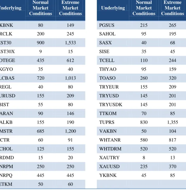
the maximum price scan range (PSR) under both normal and extreme market conditions. Table 2 shows the relevant price scan range values which indicate the maximum possible price movement during the holding period (Montgomerie-Neilson, 2012).
Table 2- Risk Parameters calculated via Historical Simulation
4.2. RISK PARAMETERS DETERMINED via EXTREME VALUE THEORY 4.2.1. Preliminary Data Analysis
The first step in econometric modeling is the data analysis (Klemens, 2009). Analyzing the events which lead high losses in case of occurrence, attention should be
Underlying Normal Market Conditions Extreme Market Conditions Underlying Normal Market Conditions Extreme Market Conditions AKBNK 80 149 PGSUS 215 265 ARCLK 200 245 SAHOL 95 195 BIST30 900 1,533 SASX 40 68 BIST30X 9 15 SISE 35 45 COTEGE 435 612 TCELL 110 244 EKGYO 35 40 THYAO 95 159 ELCBAS 720 1,013 TOASO 260 320 EREGL 40 80 TRYEUR 155 209 EURUSD 155 209 TRYUSD 145 201 FBIST 55 80 TRYUSDK 145 201 GARAN 90 146 TTKOM 70 85 HALKB 155 190 TUPRS 830 1,355 HMSTR 685 1,200 VAKBN 50 104 ISCTR 60 91 WHTANR 580 817 KCHOL 125 155 WHTDRM 520 520 KRDMD 15 20 XAUTRY 8 13 ONRPM 250 250 XAUUSD 235 370 ONRPQ 445 445 YKBNK 45 85 PETKM 50 60
concentrated on the tails where quantile-quantile plots (Q-Q plots) provides meaningful visual results in determining whether the data sample comes from a specific distribution (Dutta and Perry). Namely, the graph of the quantiles makes it possible to assess the goodness of fit of the series to the parametric model by plotting the sample against the quantiles of a theoretical reference distribution (Embrechts et al., 1999). In EVT, the sample is plotted against the exponential distribution as medium-sized tail in order to measure the fat tail behavior of the sample. If the parametric model fits the data well, the graph has the form of linear. Besides, if there is a concave line around the exponential distribution, the sample data is indicated to have fat-tail behavior; otherwise, the convex presence is indicated as being a short-tailed distribution (McNeil, 1997b).
Moreover, as a more precise criterion, the kurtosis value analyzes the tail behavior which focuses on whether the sample is heavy tailed against a normal distribution (DeCarlo, 1997). This tool measures the peakedness of a distribution relative to the normal one where excess kurtosis greater than zero implies the existence of fat tail behavior, whereas negative kurtosis value implies the thin tail behavior (Staudt, 2010).
Q-Q graphs for selected underlying on which the derivatives contracts are written in the Borsa Istanbul Futures and Options Market have been presented in Appendix- Figure 1, while the descriptive statistics including kurtosis value is in Appendix -Figure 2. Both measures indicate the existence of fat tail behavior for the sample data.
4.2.2. Determination of the Threshold Values
As a main step in Peaks over Threshold Model (POT), determination of the threshold value is performed by applying the Mean Excess Function (MEF) which is an
empirical estimation that divides the sum of the values above threshold by the number of data points which exceeds the threshold value (Gençay et al., 2001). The Mean Excess Function for a fat-tailed series is linear and tends towards infinity for high thresholds as the threshold value (u) tends towards infinity as having the positive slope (Embrechts et al., 1997).
Analyzing the Appendix -Figure 3, it can be seen that the loss values for the data sample for selected underlying in the Borsa Istanbul Derivatives Market have an upwardly rising positive trend which confirms the fat-tail behavior. Moreover, the graphs show at which point the sample tends towards positive sloping straight line which is an indicator of appropriate threshold value. For example, sample data of losses for BIST30 and GARAN is seen to have positive sloping straight lines as from the 0.030 and 0.004 values, respectively. In this way, threshold values for each underlying have been assessed by analyzing the Mean Excess Functions of the loss values of corresponding underlying with several trials.
4.2.3. Parameters and Tail Estimation
Shape and scale parameters regarding the GPD function have been estimated by applying the Maximum Likelihood Estimation (MLE). Appendix -Table 1 asserts the parameter values for different threshold values, number of observations which exceed the selected threshold values and the percentage of observation outside of the tail within the total observation as well. As it can be seen in the tables, when the threshold value increases the number observations as extreme event indicator within the tail decreases and more data is left outside of the model.
Moreover, in POT models, shape parameter with a positive value ( ) indicates the fat tail behavior of the distribution which is independent of the threshold (Mwamba et al., 2014). As it can be seen at Appendix -Table 1, the shape parameter estimated for BIST30 underlying at the threshold level of takes the 0.266 value which is quite different from zero compared with other shape parameter candidates. This also shows that distribution constituted by the values above 0.032 level has the fat-tail behavior. The same behavior is observed for other underlying which can be seen at Appendix -Table 1 as well as the other parameter values for the selected underlying.
4.2.4. Risk Parameters under EVT
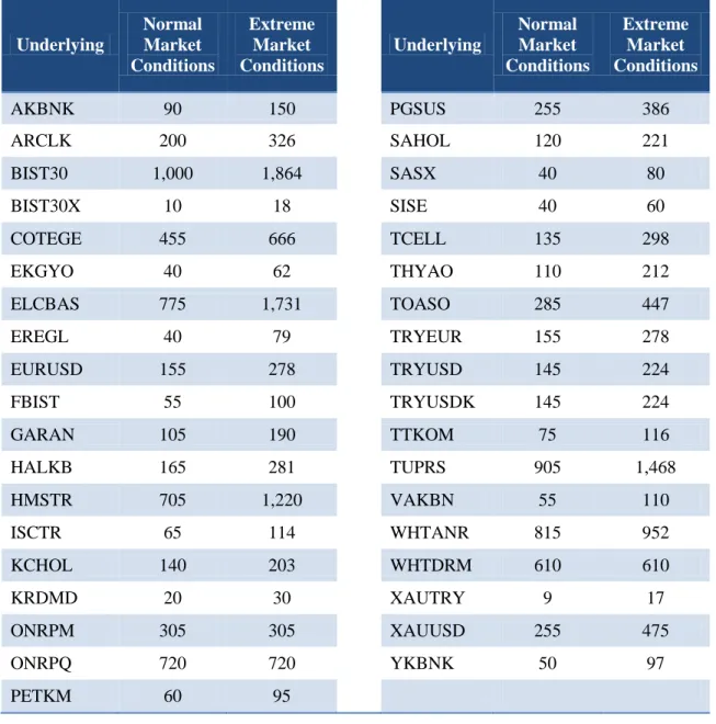
The last step in determining the risk parameters as being inputs for the initial margins of constructed portfolios which will be used in stress testing calculations is to find the maximum price scan range (PSR) values. To calculate the PSR amounts, VaR values are found by using the formula given at the 4th step of Section 3.2.2.2. For the values which reflect the fat tail behavior most dominantly, maximum price scan ranges for each underlying under both normal and extreme market conditions are presented as below Table 3.
Table 3- Risk Parameters calculated via Extreme Value Theorem
4.3. STRESS TESTING RESULTS
Risk parameters calculated under both normal and extreme market conditions with the Historical Simulation and Extreme Value Theory have been used as inputs in SPAN, which is the portfolio based margin algorithm used in Borsa Istanbul Derivatives
Underlying Normal Market Conditions Extreme Market Conditions Underlying Normal Market Conditions Extreme Market Conditions AKBNK 90 150 PGSUS 255 386 ARCLK 200 326 SAHOL 120 221 BIST30 1,000 1,864 SASX 40 80 BIST30X 10 18 SISE 40 60 COTEGE 455 666 TCELL 135 298 EKGYO 40 62 THYAO 110 212 ELCBAS 775 1,731 TOASO 285 447 EREGL 40 79 TRYEUR 155 278 EURUSD 155 278 TRYUSD 145 224 FBIST 55 100 TRYUSDK 145 224 GARAN 105 190 TTKOM 75 116 HALKB 165 281 TUPRS 905 1,468 HMSTR 705 1,220 VAKBN 55 110 ISCTR 65 114 WHTANR 815 952 KCHOL 140 203 WHTDRM 610 610 KRDMD 20 30 XAUTRY 9 17 ONRPM 305 305 XAUUSD 255 475 ONRPQ 720 720 YKBNK 50 97 PETKM 60 95
Market, and the constructed three days portfolios have been revaluated with the parameters. The potential loss which is resulted from the default of the two members with the highest exposure has been compared with the default management resources and the level of compensation has been analyzed.
Figure 6 shows the resource requirement arises from the default of two members with the highest exposure with both model and the level of cover by the existing default management resources. According to the results, EVT produces more conservative margin requirements than Historical Simulation. Moreover, while margin requirement for Day 1 can be covered by the existing default management resources with EVT model, Day 2 and Day 3 requirements can only be met by large extent. On the other hand, margin requirement amounts for all three days arisen under Historical Simulation can be easily covered by the same default management resources.
CONCLUSION
The recent global financial crisis in 2008 has once again showed that a better risk management framework and necessary tools applicable in this process are significantly important for financial stability in financial markets. While the focus in terms of risk management was mainly on banking sector at first, CCPs have also come under spotlight thanks to the role they play in capital markets and recent international regulations which extended the requirements for prudential risk management to CCPs. Accordingly, the issue has been on the agendas of regulatory bodies and practitioners as well.
In this regard, application of stress testing has been an indispensable part of the process for Central Counterparties since both the application is mandated by regulatory authorities and it sheds light on their strategic plans. Therefore, the methods to be used in such tests and the parameters to be estimated have become crucial factors to reach more realistic results.
Using Turkish derivatives market data, this study applies two methods, namely, Historical Simulation and Extreme Value Theory to undertake the stress testing and compare results. While Historical Simulation has a high popularity among practitioners, it is also used for Borsa Istanbul Derivatives Market by Takasbank as risk and collateral management body. On the other hand, Extreme Value Theory is a relatively more modern and more conservative method. It has the ability to capture extreme events within fat tails yet it is more time consuming due econometric calculations. Using three-day hypothetical portfolios which represent concentration in Turkish derivatives market, quarterly basis stress testing similar to the one that Takasbank applies to Borsa Istanbul Derivatives Market due to its function as CCP is applied. Then, the potential loss that