Detection and classification of objects and texture

(1)

DETECTION AND CLASSIFICATION OF OBJECTS

AND TEXTURE

a thesis

submitted to the department of electrical and

electronics engineering

and the institute of engineering and sciences

of bilkent university

in partial fulfillment of the requirements

for the degree of

master of science

(2)

I certify that I have read this thesis and that in my opinion it is fully adequate, in scope and in quality, as a thesis for the degree of Master of Science.

Prof. Dr. A. Enis C¸ etin(Supervisor)

Assist. Prof. Dr. Selim Aksoy

Assist. Prof. Dr. Sinan Gezici

Approved for the Institute of Engineering and Sciences:

Prof. Dr. Mehmet Baray

Director of Institute of Engineering and Sciences

(3)

ABSTRACT

DETECTION AND CLASSIFICATION OF OBJECTS

AND TEXTURE

Hakan Tuna

M.S. in Electrical and Electronics Engineering

Supervisor:

Prof. Dr. A. Enis C

¸ etin

July 2009

Object and texture recognition are two important subjects in computer vision. An efficient and fast algorithm to compute a short and efficient feature vector for classification of images is crucial for smart video surveillance systems. In this thesis, feature extraction methods for object and texture classification are investigated, compared and developed.

A method for object classification based on shape characteristics is devel-oped. Object silhouettes are extracted from videos by using the background subtraction method. Contour of the objects are obtained from these silhouettes and this 2-D contour signals are transformed into 1-D signals by using a type of radial transformation. Discrete cosine transformation is used to acquire the frequency characteristics of these signals and a support vector machine (SVM) is employed for classification of objects according to this frequency information. This method is implemented and integrated into a real time system together with

(4)

For texture recognition problem, we defined a new computationally efficient operator forming a semigroup on real numbers. The new operator does not re-quire any multiplications. The codifference matrix based on the new operator is defined and an image descriptor using the codifference matrix is developed. Texture recognition and license plate identification examples based on the new descriptor are presented. We compared our method with regular covariance matrix method. Our method has lower computational complexity and it is ex-perimentally shown that it performs as well as the regular covariance method. Keywords: : Object detection, object classification, texture classification, codif-ference matrix

(5)

¨

OZET

OBJE VE DOKU TESPITI VE SINIFLANDIRMASI

Hakan Tuna

Elektrik ve Elektronik M¨

uhendisli¯

gi B¨

ol¨

um¨

u Y¨

uksek Lisans

Tez Y¨

oneticisi:

Prof. Dr. A. Enis C

¸ etin

Temmuz 2009

Obje ve doku tanımlaması bilgisayar görü¸sü konusundaki iki önemli konudur. Resimleri sınıflandırmak i¸cin, kısa ve etkili bir nitelik vektörünü hesaplayacak yine hızlı ve etkili bir algoritma, video gözetim sistemleri i¸cin kritik bir önem ta¸sır. Bu tezde obje ve doku sınıflandırması i¸cin nitelik ¸cıkarma metodları in-celemesi, kar¸sıla¸stırması ve geli¸stirilmesi yapıldı.

S¸ekil karakteristi˘gine dayalı bir obje sınıflandırma sistemi geli¸stirildi. Arka-plan ¸cıkarımı tekni˘gi ile obje silüetleri ¸cıkarıldı. Bu silüetlerden objelerin ¸cevreleri elde edildi ve bu iki boyutlu sinyal bilgisi, bir tür dairesel dönü¸süm ile tek boyutlu sinyal bilgisine dönü¸stürüldü. Ayrık kosinüs dönü¸sümü kullanılarak bu tek boyutlu sinyallerin frekans bilgisi elde edildi ve bu frekans bilgisi ile destek¸ci vektör makineleri kullanılarak sınıflandırmaya sokuldu. Bu metod uygulamaya ge¸cirildi ve obje takibi yapan ger¸cek zamanlı bir sisteme entegre edildi.

Doku tanımlaması i¸cin, reel sayılarda verimli hesap y¨uk¨u olan ve yarı grup tanımlamasına giren yeni bir i¸slem tanımlandı. Yeni i¸slem ¸carpma i¸slemine

(6)

ve bu ortak fark matrisine dayanan bir görüntü tanımlayıcı geli¸stirildi. Bu yeni görüntü tanımlayıcıya dayanan doku tanımlama ve ara¸c plakası tespit örnekleri sunuldu. Yeni geli¸stirilen bu metod, ortak de˘gi¸sinti matrisi ile kar¸sıla¸stııldı. Kendi metodumuzun daha az karma¸sık hesap ihtiyacına ra˘gmen ortak de˘gi¸sinti matrisi ile benzer sonu¸clar verdi˘gi deneysel olarak gösterildi.

Anahtar Kelimeler: Obje tespiti, obje sınıflandırması, doku sınıflandırması, ortak fark matrisi

(7)

ACKNOWLEDGMENTS

I would like to express my gratitude to Prof. Dr. A. Enis C¸ etin for his su-pervision, suggestions and encouragement throughout the development of this thesis.

I would like to thank Assist. Prof. Dr. Selim Aksoy and Assist. Prof. Dr. Sinan Gezici for accepting to read and review this thesis.

I am also grateful to Yi˘githan Dedeo˘glu, Beh¸cet U˘gur T¨oreyin, ˙Ibrahim Onaran and Orkun Tun¸cel for their valuable contributions and comments.

I would also like to thank TUB˙ITAK-B˙IDEB for financially supporting this thesis.

Finally, I would like to express my gratitude to my family, who brought me to this stage with their endless love and support.

(8)

List of Figures

3.1 Background Subtraction; a)Background Model b)Current Frame c)Difference Function d)Thresholded difference function . . . 11 3.2 a)Object silhouette obtained from background subtraction

b)Object silhouette after image enhancement operations . . . 13 3.3 Modified radial transformation. (a) Contour of the silhouette in

fig. 3-1d, (b) corresponding 1D radial transformation . . . 15 3.4 a) Contour signal b) DCT tansformation of a . . . 16 3.5 Comparison of DCT, DFT and Wavelet decomposition in

classifi-cation by SVM . . . 17 3.6 SVM classification a) Both H1 and H2 splits two groups, H3 does

not. However, H2 has the maximum margin b) Finding the max-imum margin. . . 18 3.7 a)Aspect ratio history of the bounding rectangle of a walking

hu-man (15 frames per second), b)Circular autocorrelation of the as-pect ratio history signal . . . 20

(12)

3.8 Sample screenshots from real-time object tracking and

classifica-tion system. . . 21

4.1 Sample images from Brodatz texture database. This database contains non-homogeneus textures as well as homogeneus textures 27 4.2 Random Covariance (Codifference) Method . . . 29

4.3 Sample images from license plate database 1 . . . 32

4.4 Sample images from license plate database 2 . . . 32

4.5 Neural Network . . . 33

4.6 Sigmoid function used in neural network as an activation fuction . 34 4.7 Exponentially decreasing learning constant used in backprogation algorithm for training the neural network . . . 34

4.8 ROC curve of original covariance matrix method and codifference matrix method in license plate database 1 . . . 36

4.9 ROC curve of original covariance matrix method and codifference matrix method in license plate database 2 . . . 36

(13)

List of Tables

4.1 Comparison of success rates of each method in Brodatz texture database . . . 30 4.2 Number of train and query samples in license plate database 1 . . 33 4.3 Number of train and query samples in license plate database 2 . . 33 4.4 Overall success rates of 2 methods in the query sets of the license

plate databases . . . 35 4.5 Computational cost of the covariance and codifference methods

for a region with N pixels and M features (Division is actually not necessary for an image description applications (N − 1)c(i, j) or (N − 1)s(i, j) can be be used.) . . . 37 4.6 Simplified version of Table 4.5 assuming N M . . . 37

(14)

(15)

Chapter 1 INTRODUCTION

1.1 Overview

Video surveillance systems are getting more popular every day in monitoring security sensitive areas such as banks, highways, borders, forests etc. In gen-eral, video outputs of the more sensitive areas are processed online by human operators and the remaining video outputs are recorded for future use in case of a forensic event. However, as the number of surveillance systems increase, human operators and storage devices are becoming insufficient for operating of these systems. As the surveillance systems migrate from analog to digital sys-tems, and increase in numbers, a need for automatically interpreting the captured video arises. Increasing computational power and advances in camera systems give rise to computer aided smart video systems. Our motivation is, a computer aided video surveillance system can decrease the need for human interaction. These systems must be robust, efficient and fast in order to process real time videos.

(16)

CHAPTER 1. INTRODUCTION 2

In this research, we investigated two major subjects in computer vision. We developed and introduced new feature extraction and classification methods for object and texture recognition systems. Both methods have low computational costs, thus they are appropriate for real-time applications.

In the first part of the thesis, we introduce a system for automatically de-tecting and recognition of objects in video. By using a background model, any objects entering the scene are detected and classified. The system can be used by both grayscale and color cameras and robust to illumination changes and scale. This system is integrated and operated on a real-time video system.

The second part of the thesis covers the texture recognition problem which is another important subject in computer vision. We propose a new method for texture recognition problem by modifying a previous approach, covariance ma-trix. Covariance matrix method is lately presented by Porikli and is shown to outperform other methods in texture retrieval processes. However, for scanning large images and real time applications computational cost of covariance matrix can grow dramatically. In order to decrease the computational cost of the pro-cess, we modified the covariance equation and developed the codifference matrix method. We tested the performance of the proposed texture recognition system using the brodatz texture database and two license plate databases. Proposed method gives very good results similar to the original method in texture recog-nition experiments with a lower computational complexity and can be used as an alternative to the original method where computational cost is an important constraint.

(17)

CHAPTER 1. INTRODUCTION 3

1.2 Organization of the thesis

Organization of the thesis is as follows. In Chapter 2, we survey the previous approaches to object and texture recognition problems. In Chapter 3, we explain the proposed method for object detection and classification, and in Chapter 4, we explain our feature extraction method for texture recognition problem. Finally, Chapter 5 includes the conclusions about the thesis.

(18)

Chapter 2 RELATED WORK

2.1 Object Detection and Classification

There are many object recognition techniques proposed earlier [1-7]. In gen-eral, 2-D object recognition techniques can be classified in two major categories as statistical methods and syntactic methods. In statistical methods, a set of measurable features are extracted from the object images and the images are represented in an n-dimensional feature space. If the features extracted from image classes are distinctive, feature space is well clustered. Syntactic methods describes a set of rules in order to represent structural information of the im-ages. It has advantages in describing highly structured and complex patterns when statistical approaches are not sufficient. Statistical and syntactic methods have advantages and disadvantages over each other, and combination of these two approaches into an adaptive system is possible.

Belongie and Malik used shape context for shape matching [1]. They represent shapes by a discrete set of points sampled from the internal or external contours

(19)

CHAPTER 2. RELATED WORK 5

of the objects. Shape contexts use the relative distribution of these points. The position information of every other point relative to a chosen point are calculated in log-polar coordinates. Number of points are counted for different bins of r and φ values and this way a histogram information is extracted for every point. However, different reference points give completely different shape contexts so shape contexts with reference to every point in the shape must be calculated. This system is appropriate for template matching algorithms but they do not extract characteristic information of shapes.

Curves and skeletons are also used as shape descriptors. Curves do not give information about the interior of the objects, however they are used in so many applications effectively [2],[3]. Outline curves are used for object description with their curvature, bending angle and orientation properties. Skeletonizing, on the other hand, gives information about both the interior and outline of the shape, and also widely used [4],[5]. Sebastian and Kimia have a good comparison of these two shape descriptors in the literature [6]. Skeletons have a better performance in shape retrieval experiments than the curves, together with a drawback on the computational cost.

Serre and Pogio simulated human visualization by using a multilayer neural network [7]. Image scenes are filtered with a set of gabor filters, local maximas of filter responses are used as feature sets. Of course these are very computationally heavy operations which are not appropriate for real-time applications.

(20)

2.2 Texture Detection and Classification

Texture recognition and classification is a widely studied subject in computer vision. There are several well documented studies in the literature. Most of the works have focused on finding good features for texture retrieval process.

Haralick proposed occurrence matrix, which is also referred to as a co-occurrence distribution [8]. In this method, distribution of co-occurring values in an image at a given offset are calculated in order to form a co-occurrence matrix, and several features are extracted from this matrix for texture recognition task. Co-occurrence matrix is sensitive to spatial frequencies of the texture, however it is not recommended for textures with large primitives.

Statistical features of textures are also used for classification. Antoniades and Nandi used second and third order statistics directly for differentiate texture images [9]. The classification ability of the system is very primitive and can not be used to differentiate a large database of texture images.

Gabor filtering is another widely used approach in texture recognition [10],[11],[12]. Qaiser et.al fuses gabor and moment energy features of textures for a better texture recognition [13]. Fusing two different approaches gives better results than individual ones.

Lin, Wang and Yang adopt a structural approach for texture retrival from an image database, rather than using frequency domain methods [14]

There are several feature extraction techniques for texture categorization, recognition and classification tasks. Ma and Zhang has a well prepared survey about different feature extraction methods for image retrieval and comparison of their performances [15].

(21)

Recently, Porikli and et.al. introduced covariance matrix as a new region descriptor for texture recognition task [16]. Covariance matrix is shown to out-perform previous feature extraction methods in several texture retrieval and clas-sification experiments.

(22)

Chapter 3 OBJECT DETECTION AND

CLASSIFICATION

Object detection and classification system is composed of an object detection system based on background subtraction method and a classification system based on shape features. So it has both advantages and disadvantages of these systems.

The system comprises of three main steps

1. Object detection 2. Feature extraction 3. Object classification

First step includes detection of the pixels that the object lays on. We use background subtraction method for discriminating the background pixels from the foreground pixels which contains the objects of interest. This way, any new

(23)

CHAPTER 3. OBJECT DETECTION AND CLASSIFICATION 9

object entering the scene is detected by using the difference image between the background model and the current frame. From the difference image, object shapes are obtained.

In the second step, we use the boundaries of the objects for feature extrac-tion. We extract the contour points from the black and white silhouettes, take the modified radial function (MRF) of these contour signals and transform these signals into the frequency domain. We investigate DCT (Discrete Cosine Trans-form), DFT (Discrete Fourier Transform) and Wavelet Transformation of these signals and use the coefficients of these transformations in classification step.

Third step includes the classification of objects by using these features. This step employs an SVM(support vector machine) algorithm. Each transformation is experimented and success rates are compared.

3.1 Object Detection

The first step of the program is to detect the regions where object occupies in the image and extract the shape information of these objects. We used background subtraction method in order to distinguish the object from the background im-age. After using morphological operations and noise removal, blob of the object silhouette is extracted from the image by using connected component analysis.

3.1.1 Background Subtraction

Background subtraction is a widely used method for discriminating the back-ground from the objects of interest [17]. Foreback-ground pixels are basically detected

(24)

by subtracting the current frame pixel-by-pixel from a background model. The pixels with a difference higher than a threshold value is classified as foreground pixels; and the pixels with a difference lower than this threshold value is classi-fied as background pixels. Figure 3.1 depicts a sample background subtraction operation.

Background subtraction is known to perform well in static backgrounds. It is very sensitive to the changes in the illumination. However, in order to overcome this situation and decrease the sensitivity of method for illumination changes, background model can be updated with every new frame.

A pixel in the current frame at location (x, y) and at time t is denoted by It(x, y), and the pixel in the background model updated at time t, at location

(x, y) is denoted as Bt(x, y).So, It(x, y) is considered as a foreground pixel if

|It(x, y) − Bt(x, y)| ≥ τ (3.1)

where τ is a pre defined threshold. We use pixels below this predefined threshold in the background update. This way, foreground pixels in which detected object lays on do not effect the background model. Background model is updated with the following function.

Bt+1 = αIt+ (1 − α)Bt (3.2)

Selection of these parameters has a significant effect on the performance of the system. High threshold values cause misdetection of the objects in the scene, or cavities in the object silhouette. On the other hand, lower threshold values cause a noisy output. Background model update also should be handled carefully. If the update parameter α is too high, objects in the scene may corrupt the background model, while if it is too low, system becomes too sensitive to illumination changes in the scene.

(25)

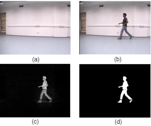
Figure 3.1: Background Subtraction; a)Background Model b)Current Frame c)Difference Function d)Thresholded difference function

3.1.2 Image Enhancement

The difference function between the current frame and the background model is not sufficient to extract the silhouettes of the objects. Noises in the difference image caused by camera noise or changes in the ilumination must be handled accordingly. Also similarities between the background model and the object texture may cause some occlusions on the image silhouette.

The first step for removing nosie in the image is to apply a threshold value. Thus, before proceeding, difference image is thresholded by a constant value and transformed to a binary image. This threshold value is determined manually

(26)

according to the response of the difference image. If this threshold value is low, then we obtain an image with a high level of noise. On the other hand, if this threshold value is chosen to be high, then some occlusions or holes can occur in the image. This second condition is very crucial because object silhouettes can split into two or more parts which will totally change the shape information. Therefore we limit the threshold value where occlusions are pretty small with respect to the object silhouette and deal with noise in the background pixels in further steps.

After using a threshold value, we obtain a binary image with black (back-ground pixel) and white (fore(back-ground pixel) pixels. We use morphological oper-ations in order to remove noise and holes in the image. (erode, dilate, opening, closing). Opening removes small noises from the background image and closing removes small occlusions in the foreground image.

We use connected component analysis in order to obtain object silhouettes in the image. Very small components are neglected as a last noise removal step and objects big enough are saved for further processing.

Figure 3.2 shows the difference image and the resultant image after image enhancement operations.

3.2 Feature Extraction

In this step we start with black and white silhouettes of the detected objects. From the black and white silhouettes, the contour points of the objects are ex-tracted. We take the modified radial transformation of these contour points and then transform the obtained signal to the frequency domain.

(27)

Figure 3.2: a)Object silhouette obtained from background subtraction b)Object silhouette after image enhancement operations

3.2.1 Modified Radial Transformation

The rectangular coordinates of contour points obtained from the contour ex-traction step are not suitable for representation of object shapes, because this coordinate representation is not invariant to rotation and scale. Also, because 2-D contour information is hard to employ, we should reduce the dimension of contour information. An alternative method for this is to use radial transforma-tion. This transformation uses the idea that, every point on the boundary can be approximated as a vector projected between a reference point and the point on the boundary. Thus, the points on the boundary of an object are represented with r and φ values instead of x and y, where r corresponds to the distance between the reference and the boundary point, and φ coresponds to the angle between the radial vector and a reference axis. If we increase φ with equal angles and record r(φ), we obtain a 1 dimensional signal which also has the rotation invariance property. This representation has been used in many applications [18],[19].

(28)

However, radial transformation outputs multiple values when the radial vec-tors intersects the boundary more than once. In these cases, radial function must be modified or must be handled carefully in order to represent object contours. In order to overcome this situation, we use modified radial function (MRF) which was proposed earlier in [20].

In modified radial function, we do not take the angularly equispaced points on the contour, instead we move on the contour arc with equal distance values and project the vector from the reference point to these points on the boundary. This way, modified radial function (MRF) represents the distance and angle components with respect to another parameter l, where l corresponds to the arc length from a reference starting point to the point on the boundary. In this transformation, we both have a distance component r(l) and angle component φ(l) for a full representation of the contour points. However, in our method we do not take the angle component φ(l) and continue only with the distance component r(l).

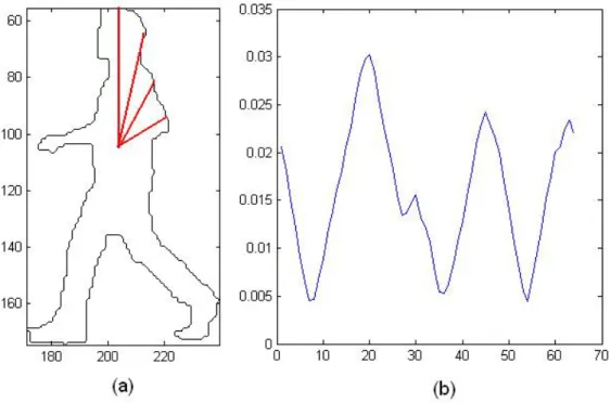
We generally set the starting point on the boundary as the top left corner of the contour and the reference point as the centroid of the object contour. Since the increments of l are not usually equally-spaced, we used linear interpolation to take exactly 64 samples from every contour.

In order to gain scale robustness, we scale the data such that the area under the graph is always constant. Therefore we end up with a normalized 64-point data signal. The MRF of the silhouette obtained in object detection step is depicted in figure 3.3.

(29)

Figure 3.3: Modified radial transformation. (a) Contour of the silhouette in fig. 3-1d, (b) corresponding 1D radial transformation

3.2.2 Discrete Cosine Transformation

Discrete Cosine Transform (DCT) is a linear, invertible transformation which expresses discrete signals in terms of a sum of cosines with different amplitudes and frequencies. Discrete cosine transformation is conceptually very similar to Discrete Fourier Transformation (DFT). However it uses only real coefficients on the contrary to Fourier transform, which uses complex coefficients.

The mathematical formula for discrete cosine transformation is

y(k) = w(k) N X n=1 x(n)cosπ(2n − 1)(k − 1) 2N , k = 1, ..., N (3.3) where

(30)

CHAPTER 3. OBJECT DETECTION AND CLASSIFICATION 16 w(k) =    1 √ N, k = 1 2 √ N, 2 ≤ k ≤ N    (3.4)

DCT has a strong energy compaction property, i.e. it does a better job in concentrating the energy in the lower order coefficients [21]. Thus, it has a very wide usage in data compression of image and audio.

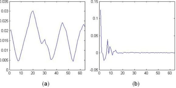
We used DCT in order to extract the frequency information of the contour signals. Figure 3.4 shows the DCT of a contour signal. The characteristic features of contour signals are mainly compensated in the lower frequency bands. There-fore we took first 10 coefficients (except the very first one, which corresponds to DC component of the signal and always constant because of the normalization) as the feature vector for each shape.

Figure 3.4: a) Contour signal b) DCT tansformation of a

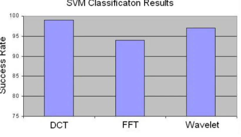
We compared DCT with DFT and wavelet decomposition. We took the 10 coefficients from the same frequency bands for each method. We used Haar wavelet for wavelet decomposition.

(31)

Figure 3.5 shows the results of our comparisons. We used three different object classes as human, human group and vehicle. Train set consists of 57 human, 58 human group and 38 vehicle pictures. Test set consists of 56, 64 and 35 images for human, human group and vehicle object groups respectively.

Figure 3.5: Comparison of DCT, DFT and Wavelet decomposition in classifica-tion by SVM

3.3 Object Classification

Object classification step is done by a support vector machine (SVM) algorithm.

3.3.1 Support Vector Machines

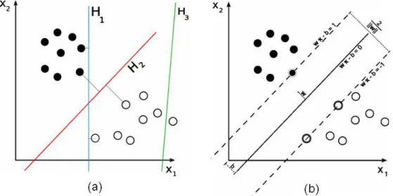
Support Vector Machines (SVMs) are a type of linear classifiers. SVM uses su-pervised learning methods, and can be used for both classification and regression. Suppose we have two class input data in an N dimensional feature space. Sup-port vector machines try to find an N − 1 dimensional hyperplane which divides the space into two and separates these two groups from each other. However,

(32)

there are probably lots of hyperplanes which splits these two groups. Thus, additionally, support vector machines try to find the hyperplane such that the distance from the closest points from each class to this hyperplane is at maxi-mum. This hyperplane is called the maximum margin hyperplane. Figure 3.3.1 displays these hyperplanes.

We used libsvm library which is widely known and used in classification tasks [22]. We used one model for three classes with RBF(radial basis function) kernel.

Figure 3.6: SVM classification a) Both H1 and H2 splits two groups, H3 does not. However, H2 has the maximum margin b) Finding the maximum margin.

(Images are taken from wikipedia.org internet site)

3.4 Real-Time object detection, tracking and

classification system

We integrated our object classification system with a real-time object detection and tracking system [23].

(33)

We used three object categories, human, human group and vehicle. Our method showed very good performance in classification of different objects. Er-rors occur generally because of the improper silhouette extraction in the back-ground subtraction step.

Results of the background subtraction method has a crucial importance in the results of the overall system. Even we achieve to obtain very good results in our experiments, improperly extracted object silhouettes sometimes may corrupt the results. In order to obtain a better classification, we added simple rules into the classification step of the final system.

First, human classes generally have the lowest values of aspect ratio because of their shapes. So we used a threshold value on the aspect ratio of the detected objects. If the detected object has a lower aspect ratio than this threshold, we decided that this object is a human.

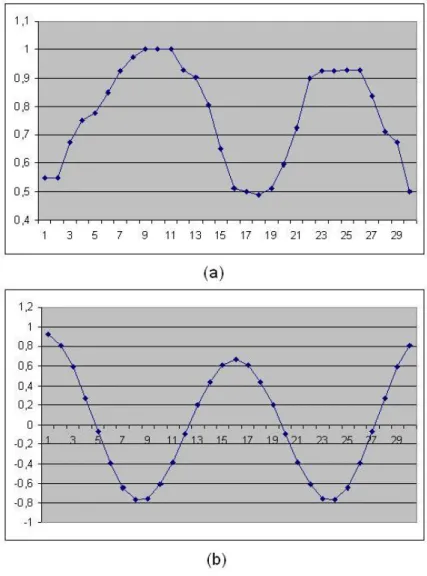
Aspect ratios of bounding rectangles of walking human silhouettes compose a periodical signal, which is very distinctive from other object classes. We recorded the aspect ratio history of detected objects and found the periodicity by using autocorrelation of the signals (Figure 3.7).

X(i) = N X n=0 (x(n) − µx)(x(mod(n − i, N )) − µx) (3.5) where µx = 1 N N X n=0 x(n) (3.6)

In our experiments, we saw that walking human signals produce aspect ratio signals with periodicity with 0.8-1.2 seconds. So, if the detected object is moving and if we find peaks in the autocorrelation function in this range with a value

(34)

above a certain threshold, system decides that the detected object is indeed a human. Human group and vehicle classes do not produce a periodical signal, instead they produce a chaotic behavior.

Figure 3.7: a)Aspect ratio history of the bounding rectangle of a walking human (15 frames per second), b)Circular autocorrelation of the aspect ratio history signal

If the detected object passes these simple classification rules, SVM is em-ployed for classification task.

We also used temporal information of the detected objects in classification. By using tracking system, we recorded the previous results of object detection.

(35)

If the detected object does not collide with or detach from another object, we use the previous results of object detection together with the last result to vote for object class. Basically, we used results from 2 previous frames and the current frame. If the previous 2 results agrees with each other but do not agree with the current result, we output the most voted result.

Figure 3.8: Sample screenshots from real-time object tracking and classification system.

(36)

Chapter 4 TEXTURE RECOGNITION

Texture is one of the main characteristics for analysis of images, and texture recognition is a very important subject in computer vision. A fast and efficient algorithm for texture description is a vital issue.

We present a new method for texture recognition problem by modifying a previous approach, covariance matrix, and decreasing the computational cost. We call it as codifference matrix. In this proposed method, the multiplication operation of the well-known covariance method is replaced by a new operator. The new operator does not require any multiplications. Codifference matrix method is shown to perform as well as the original previous method, and even outperform the previous one in some tests. Texture recognition and license plate identification examples are presented based on this method.

(37)

CHAPTER 4. TEXTURE RECOGNITION 23

4.1 Covariance Matrix as a Region Descriptor

Porikli et.al introduced the covariance matrix method as a new image region descriptor, and showed that covariance matrix method performed better than the previous approaches to the texture recognition problem [16, 24]. They also developed an object tracking method using the covariance matrix [25].

4.1.1 Covariance Matrix

Covariance is the measure of how two variables behave according to each other. If the variables tend to vary together, (if one of them is above its expected value when the other one is also above its expected value), the covariance is positive, the covariance is negative if the variables tend to vary inversely (one of them is above its expected value while the other one is below its expected value). The mathematical expression of covariance is as follows

cov(a, b) =

N

X

k=1

(ak− µa)(bk− µb) (4.1)

If we have n variables α1, α2,... αN, covariance matrix of these variables is

defined as C =         

cov(α1, α1) cov(α1, α2) · · · cov(α1, αN)

cov(α2, α1) cov(α2, α2) · · · cov(α2, αN)

..

. ... . .. ... cov(αN, α1) cov(αN, α2) · · · cov(αN, αN)

         (4.2)

(38)

Let f be a d-dimensional feature vector for each pixel I(x, y) of a two-dimensional image.

F (x, y) = φ (I, x, y) (4.3) where φ is the feature mapping such as the intensity, gradient or a filter response of the pixel. Let us index the image pixels using a single index k, and assume that there are n pixels in a given image region. As a result we have n d-dimensional feature vectors (fk)k=1...n. The covariance matrix of the image

region is defined as C = 1 n − 1 n X k=1 (fk− µ) (fk− µ) T (4.4)

where µ is the mean vector of the feature vectors.

For d chosen features, we will obtain a dxd covariance matrix. However, since cov(x, y) = cov(y, x)

covariance matrix is symmetric, and since

cov(x, x) = var(x)

diagonal elements of the covariance matrix are actually variances of chosen fea-tures in the region. Thus, for n different feafea-tures, we will have n(n+1)/2 different values in the covariance matrix for computation.

(39)

4.2 Codifference Matrix

Computational cost of a single covariance matrix for a given image region is not heavy. However, computational cost becomes important when we want to scan a large image at different scales and all locations to detect a specific object. Furthermore, many video processing applications require real-time solutions. In order to decrease the computational cost, we modified the core function of co-variance equation (equation 4.5) and obtained codifference equation (equation 4.6) C(a, b) = 1 n − 1 n X k=1 (a − µa) (b − µb) (4.5) S(a, b) = 1 n − 1 n X k=1 (a − µa) (b − µb) (4.6)

where the operator acts like a matrix multiplication operator, however, the scalar multiplication is replaced by an additive operator ⊕. The operator ⊕ is basically an addition operation but the sign of the result behaves like the multiplication operation: a⊕ b =                  a + b, if a ≥ 0 and b ≥ 0 a − b, if a ≤ 0 and b ≥ 0 −a + b, if a ≥ 0 and b ≤ 0 −a − b, if a ≤ 0 and b ≤ 0 (4.7)

for real numbers a and b. We can also express Equation 4.7 as follows

a ⊕ b = sign (a × b) (|a| + |b|) (4.8) or in a more straigtforward mathematical expression

(40)

a⊕b = a · b

|a| · |b|(|a| + |b|) (4.9) Our codifference equation behaves similar to original covariance function. If the variables tend to vary together, codifference equation gives positive results as the original equation, if variables tend to vary inversely, codifference equation gives negative results as the original equation. Also since S(x, y) = S(y, x), cod-ifference matrix is symmetric as covariance matrix. On the other hand, compu-tational cost is decreased by replacing the multiplication operation with addition operation.

Operator ⊕ satisfies totaliy, associativity and identity properties i.e. it is a monoid function. In other words it is a semigroup with identity property.

4.3 Texture Classification

We use well known Brodatz texture database for texture classification tests. We repeat the same steps with the method described in [16], however we use codif-ference matrix as a region descriptor instead of covariance matrix, and compare the results of two different image description methods. The classification proce-dure we followed in these experiments is not computationally efficient, however these texture classification experiments give a good comparison on a well known database between the original and the modified methods.

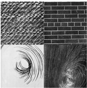
The Brodatz texture database which we used in our experiments consists of 111 texture images. The size of each image is 640 x 640. Classification is a challenging task because of the non homogeneous texture images in the database. Sample images from Brodatz texture database is shown in figure 4.1. In our

(41)

experiments, we divide each texture image into 320 x 320 sized four sub-images. Two of these images are used for training and the remaining two are used for testing.

Figure 4.1: Sample images from Brodatz texture database. This database con-tains non-homogeneus textures as well as homogeneus textures

4.3.1 Covariance Features

In texture classification step, we use 5 different features extracted from texture images. These are intensity values of pixels and the norms of first and second order derivatives of intensity values of pixels in both x and y directions. Feature vector is defined as

(42)

Therefore every pixel in a given image region is mapped to a d = 5-dimensional feature vector. Then the covariance and the codifference of these features are calculated using both Eq. (4.5) and Eq. (4.6), respectively. As a result, we end up with 5x5 dimensional covariance and codifference matrices, representing each region.

4.3.2 Random Covariance(Codifference) method

For representation of each texture image, we choose 100 regions from random locations in the image. Each region is a square box with random sizes which varies from 16x16 to 128x128. We calculate the covariance and the codifference matrices of each region. Thus, every texture subimage is represented with 100 covariance and 100 codifference matrices extracted from random regions of these images. Since we have 2 subimages from the same texture image, we will have 200 covariance and codifference matrices representing each texture. Figure 4.2 depicts the random covariance(codifference) matrix method.

4.3.3 K-nearest neighbor algorithm

For classification task, we employ k-nearest neighbor algorithm.

K-nearest neighbor algorithm (k-NN) is a supervised learning method which classifies samples according to majority of the closest training samples in the feature space.

We use a generalized eigenvalue based distance metric to compare covariance and codifference matrices which was introduced in [26] [27] and used in [16] as a

(43)

Figure 4.2: Random Covariance (Codifference) Method part of the k-NN method:

d(C1, C2) = v u u t n X k=1 ln2_λ i(C1, C2) (4.11)

λi(C1, C2) is the generalized eigenvalues of matrices C1 and C2. Distance

function is a metric, i.e. it satisfies the following conditions

1. Positivity: d(A, B) > 0 and d(A, B) = 0 only if A = B. 2. Symmetry: d(A, B) = d(B, A).

(44)

We measure the distances between the instance covariance matrix to be clas-sified and the covariance matrices in the train database. k nearest samples from the train database is chosen and the query instance is assigned to the class most common amongst these k samples from the train database. If k = 1, then the query instance is assigned to the class of its nearest neighbor.

The choice of k depends on the data. Large values of k with respect to the number of samples decrease the probability of misclassifying and decrease the effect of noise. However it makes the classification boundary less distinct.

4.3.4 Classification Results

Brodatz texture database is a challenging database with lots of non-uniform texture images. For comparison of our codifference matrix method with the original covariance matrix method, we choose 100 randomly sized regions from random locations from each image in the train set. Covariance and codifference matrices are extracted from these random regions and added to the train set. Then the same procedure is repeated for composing the query set. For different values of k, samples in the query set are classified by using k-nn algorithm in both covariance and codifference feature space. Results are listed in Table 4.1 Table 4.1: Comparison of success rates of each method in Brodatz texture database

Covariance Matrix Codifference Matrix k=5 213/222 209/222 %95.9 %94.1 k=10 214/222 215/222 %96.3 %96.8 k=20 214/222 215/222 %96.3 %96.8 30

(45)

In [16], covariance method seems to achive better results in Brodatz texture database. However, since each texture is represented by covariance and codiffer-ence matrices extracted from random locations, these small differcodiffer-ences in results are possible.

4.4 Plate Recognition

Porikli also used covariance matrix method for license plate recognition problem [28]. In order to compare our codifference matrix with Porikli’s method, we test two methods with two different license plate database.

4.4.1 License Plate Databases

First license plate dataset contains plate images gathered from an internet page which contains galleries of used cars for sale (arabam.com). License plate images taken from this website have different illumination, are at different scales and taken from different angles. That is to say, this dataset is a challenging dataset. This database contains Turkish license plate samples. Some sample images from this database is shown in figure 4.3.

The second dataset is taken from Porikli’s dataset with his permission. It is very similar to the dataset used in [28] except the negative samples since negative samples are taken randomly from non-plate regions in car images. The license plate images in this database have different illumination, however they are taken at similar angles and are at the same scale. This dataset contains license plates images from USA. Some sample images from this database is shown in figure 4.4.

(46)

Figure 4.3: Sample images from license plate database 1

Figure 4.4: Sample images from license plate database 2

The negative samples for train and query datasets are obtained randomly from car pictures with blackened or removed license plates. In order to simulate real life conditions, we use greater number of negative samples with respect to the number of positive samples, in both train and test stages.

4.4.2 Matrix Coefficients

The covariance and codifference matrix coefficients used in this problem contains 7 features. x and y corresponds to the rectangular coordinates of the pixels, I corresponds to the intensity value, and Ix, Iy, Ixx, Iyy corresponds to the first

and second order derivatives of intensity values.

C = [ |x| |y| |I| |Ix| |Iy| |Ixx| |Iyy| ] (4.12)

x and y values are all normalized to [0 1], in order to gain scale robustness in images. Therefore cov(x, x),cov(y, y) and cov(x, y) values are always constant for

(47)

Table 4.2: Number of train and query samples in license plate database 1 Database I

Positive Samples Negative Samples

Train 99 800

Query 90 800

Table 4.3: Number of train and query samples in license plate database 2 Database II

Positive Samples Negative Samples Train 240 2400 Query 173 1730

all images. So, for 7 features shown in equation 4.12, we end up with 25 different covariance values.

4.4.3 Classification by Neural Network

We employ a three layer neural network algorithm for classification task. Neural network outputs a numerical result in the range [-1,1] to decide if the region corresponds to a license plate or not.

Our neural network consists of three layers, input layer, hidden layer and the output layer. We used 25 neurons in the input and hidden layers as the size of the input vector. There is only 1 neuron in the output layer for computing the result of the neural network. Our neural network uses supervised learning and backpropagation algorithm for training.

(48)

The neural network uses a sigmoid function in equation 4.13 tansig(z) = 2

1 + e−2z − 1 (4.13)

Figure 4.6: Sigmoid function used in neural network as an activation fuction We use exponentially decreasing learning constant c, as the number of itera-tions increase.

c = 0.1ei/1000 (4.14)

Figure 4.7: Exponentially decreasing learning constant used in backprogation algorithm for training the neural network

For training phase, we use samples from each class, license plate images and non license plate images. Pixel-wise features of these images are computed and covariance and codifference matrices are formed from these values. Non-repeating and non-constant values are removed and the remaining coefficients are used for

(49)

forming the feature vector of each image. Then with -1 and 1 labels respec-tively for non plate and plate images, these feature vectors are fed to the neural network. A feed-forward back propagation algorithm is used for updating the weight matrices.

4.4.4 Classification Results

We use a threshold on the result of the neural network in order to decide if the query image corresponds to a plate or not. Since output is in the range [-1 1], this threshold value is 0 by default. Table 4.4 presents the results of two methods. Table 4.4: Overall success rates of 2 methods in the query sets of the license plate databases

Database 1 Database 2 Covariance Matrix % 96.4 %99.0 Codifference Matrix % 97.3 %99.3

In order to obtain ROC curves, we ordered the query samples according to the output values of the neural network. We divide this ordered sequence from every possible location. Than the part with higher values are labeled as positive results and the part with lower values are labeled as negative results. At each different division, number or true positives and true negatives are computed and marked on the ROC graph. In other words, we changed the threshold value between -1 to 1 and plot the success rates for positive and negative success rates. As we move right-down on the ROC curves, the threshold value decreases, as we move left-up on the ROC curves, threshold value increases. Figure 4.8 and figure 4.9 represent the ROC curves of two methods in the first and in the second license plate databases respectively.

(50)

Figure 4.8: ROC curve of original covariance matrix method and codifference matrix method in license plate database 1

Figure 4.9: ROC curve of original covariance matrix method and codifference matrix method in license plate database 2

Results show that our codifference matrix descriptor gives very similar results to original covariance matrix descriptor. Also, modified method has a lower computational cost advantage over the original one.

(51)

4.5 Computational Cost Comparison

The computational cost of the codifference method is lower than the covariance method because it does not require any multiplications. This is especially im-portant in real time applications in which the entire image or video frame has to be scanned at several scales to determine matching regions and ASIC imple-mentations [29, 30, 31].

Table 4.5 describes the computational cost of the covariance method and the codifference method for an image region having N pixels. Each pixel has M features. Therefore the resulting covariance and codifference matrices are M by M . Table 4.6 is a simplified version of the table 4.5 assuming N M .

Table 4.5: Computational cost of the covariance and codifference methods for a region with N pixels and M features (Division is actually not necessary for an image description applications (N − 1)c(i, j) or (N − 1)s(i, j) can be be used.)

Covariance Matrix Codifference Matrix Sum 3M2N +N M −M₂ 2−M 4M2N +2N M −M₂ 2−M Multiplication M2₂+MN 0

Sign Comparison 0 M2₂+MN Division M2₂+M M2₂+M

Table 4.6: Simplified version of Table 4.5 assuming N M Covariance Matrix Codifference Matrix Sum 3M2₂+MN 4M2₂+2MN Multiplication M2₂+MN 0 Sign Comparison 0 M2₂+MN

(52)

Chapter 5 CONCLUSIONS

In this thesis, we studied feature extraction methods for recognition and classi-fication of objects and texture in images.

Object detection and recognition system is designed for real time video sys-tems. We integrated our object classification system with a real-time object detection and tracking system and operated in real time videos. The system uses shapes of the objects for classification. Therefore it is robust against the color and texture of the detected objects. However, it is very sensitive to im-proper extraction of the object silhouettes, which makes it more appropriate for static indoor environments or for outdoor environments with limited view, like parking lots, stations etc. The system can be upgraded by adding color and texture information for better classification results.

For texture classification system, we modified a previous approach, covari-ance matrix, by lowering its computational cost. We call this new matrix as codifference matrix. Using a commonly used brodatz texture database and two license plate picture databases, we compared the covariance and the codifference

(53)

CHAPTER 5. CONCLUSIONS 39

matrix methods. Experiments show that modified method performs as well as the original method with a lower computational complexity. It can be used in embedded systems with a limited computational power or in ASIC (Application Specific Integrated Circuit) implementations more efficiently than the original method.

(54)

Bibliography

[1] J. M. Serge Belongie, “Shape matching and object recognition using shape contexts,” IEEE Transactions on Pattern Analysis and Machine Intelli-gence,AVSS, vol. 7, pp. 1832–1837, 2005.

[2] L. Younes, “Computable elastic distances between shapes,” SIAM J. Appl. Math, vol. 58, pp. 565–586, 1998.

[3] E. Milios and E. G. M. P. Y, “Shape retrieval based on dynamic program-ming,” IEEE Transactions on Image Processing, vol. 9, pp. 141–146, 2000. [4] S. Zhu and A. Yuille, “Forms: a flexible object recognition and modelling

system,” IEEE International Conference on Computer Vision, vol. 0, p. 465, 1995.

[5] K. Siddiqi, A. Shokoufandeh, S. J. Dickinson, and S. W. Zucker, “Shock graphs and shape matching,” in ICCV ’98: Proceedings of the Sixth Inter-national Conference on Computer Vision, (Washington, DC, USA), p. 222, IEEE Computer Society, 1998.

[6] T. B. Sebastian and B. B. Kimia, “Curves vs skeletons in object recogni-tion,” in In IEEE International Conference of Image Processing, pp. 247– 263, 2001.

(55)

BIBLIOGRAPHY 41

[7] T. Serre, L. Wolf, S. Bileschi, M. Riesenhuber, and T. Poggio, “Robust ob-ject recognition with cortex-like mechanisms,” IEEE Transactions on Pat-tern Analysis and Machine Intelligence, vol. 29, pp. 411–426, 2007.

[8] R. M. Haralick, K. Shanmugam, and I. Dinstein, “Textural features for image classification,” IEEE Transactions on Systems, Man and Cybernetics, vol. 3, no. 6, pp. 610–621, 1973.

[9] V. Antoniades and A. Nandi, “Texture recognition or classification using statistics,” IEEE Colloquium on Applied Statistical Pattern Recognition, pp. 10/1–10/6, 1999.

[10] Y. Hongyu, L. Bicheng, and C. Wen, “Remote sensing imagery retrieval based-on gabor texture feature classification,” Proceedings of 7th Interna-tional Conference on Signal Processing, vol. 1, pp. 733–736, 2004.

[11] I. J. Sumana, M. M. Islam, D. Zhang, and G. Lu, “Content based image retrieval using curvelet transform,” in MMSP, pp. 11–16, IEEE Signal Pro-cessing Society, 2008.

[12] G. Gimel’Farb and A. Jain, “On retrieving textured images from an image database,” Pattern Recognition, vol. 29, pp. 1461–1483, September 1996. [13] N. Qaiser, M. Hussain, N. Qaiser, A. Hanif, S. M. J. Rizvi, and A. JaIi,

“Fusion of optimized moment based and gabor texture features for better texture classification,” Proceedings of 8th International Multitopic Confer-ence, pp. 41–48, 2004.

[14] H. Lin, L. Wang, and S. Yang, “Regular-texture image retrieval based on texture-primitive extraction,” Image and Vision Computing, vol. 17, pp. 51– 63, January 1999.

(56)

BIBLIOGRAPHY 42

[15] W.-Y. Ma and H. J. Zhang, “Benchmarking of image features for content-based retrieval,” Conference Record of the Thirty-Second Asilomar Confer-ence on Signals, Systems and Computers, vol. 1, pp. 253–257, November 1998.

[16] F. O.Tuzel and P.Meer, “Region covariance: A fast descriptor and for de-tection and classification,” in Proc. of Image and Vision Computing, (Auck-land, New Zeland), 2004.

[17] A.M.McIvor, “Background subtraction techniques,” in Proc. of 9th Euro-pean Conf. on Computer Vision, vol. 2, (Graz, Austria), pp. 589–600, May 2000.

[18] D. Chetverikov and A. Lerch, “A multiresolution algorithm for rotation-invariant matching of planar shapes,” Pattern Recogn. Lett., vol. 13, no. 9, pp. 669–676, 1992.

[19] B. Jawerth and W. Sweldens, “An overview of wavelet based multiresolution analyses,” SIAM Rev., vol. 36, no. 3, pp. 377–412, 1994.

[20] W. B. Quang Minh Tieng, “Recognition of 2d object contours using the wavelet transform zero-crossing representation,” Pattern Analysis and Ma-chine Intelligence, vol. 19, no. 8, pp. 910–916, 1997.

[21] K. R. Rao and P. Yip, Discrete Cosine Transform: Algorithms, Advantages, Applications. Academic Press, Boston, 1990.

[22] C.-C. Chang and C.-J. Lin, LIBSVM: a library for support vector ma-chines, 2001. Software available at http://www.csie.ntu.edu.tw/~cjlin/ libsvm.

[23] Y. Dedeo˘glu, Moving Object Detection, Tracking and Classification for Smart Video Surveillance. PhD thesis, Bilkent University, 2004.

(57)

BIBLIOGRAPHY 43

[24] F. Porikli, “Making silicon a little bit less blind: Seeing and tracking hu-mans,” SPIE OE Magazine, Newsroom Edition, 2006.

[25] F. Porikli, ¨O. T¨uzel, and P. Meer, “Covariance tracking using model update based means on riemannian manifolds,” in Proc. IEEE Conf. on Computer Vision and Pattern Recognition, 2006.

[26] W. F¨orstner and B. Moonen, “A metric for covariance matrices,” technical report, Dept.of Geodesy and Geoinformatics, Stuttgart University, 1999. [27] J. Br¨ummer and L. Strydom, “An euclidean distance measure between

co-variance matrices of speechcepstra for text-independent speaker recogni-tion,” in Proceedings of the South African Symposium on Communications and Signal Processing, pp. 167–172, 1997.

[28] T. K. Fatih Porikli, “Robust license plate detection using covariance de-scriptor in a neural network framework,” IEEE International Conference on Advanced Video and Signal Based Surveillance, AVSS, p. 107, 2006.

[29] K. Benkrid, “A multiplier-less fpga core for image algebra neighbourhood operations,” in Proceedings of IEEE International Conference on Field-Programmable Technology, pp. 294–297, Dec 2002.

[30] H. Jeong, J. Kim, and W. kyung Cho, “Low-power multiplierless dct ar-chitecture using image correlation,” IEEE Transactions on Consumer Elec-tronics, vol. 50, pp. 262–267, Feb 2004.

[31] T. Tran, “The bindct: fast multiplierless approximation of the dct,” IEEE Signal Processing Letters, vol. 7, pp. 141–144, Jun 2000.

Detection and classification of objects and texture

DETECTION AND CLASSIFICATION OF OBJECTS

AND TEXTURE

a thesis

submitted to the department of electrical and

electronics engineering

and the institute of engineering and sciences

of bilkent university

in partial fulfillment of the requirements

for the degree of

master of science

ABSTRACT

DETECTION AND CLASSIFICATION OF OBJECTS

AND TEXTURE

Hakan Tuna

M.S. in Electrical and Electronics Engineering

Supervisor:

Prof. Dr. A. Enis C

¸ etin

July 2009

¨

OZET

OBJE VE DOKU TESPITI VE SINIFLANDIRMASI

Hakan Tuna

Elektrik ve Elektronik M¨

uhendisli¯

gi B¨

ol¨

um¨

u Y¨

uksek Lisans

Tez Y¨

oneticisi:

Prof. Dr. A. Enis C

¸ etin

Temmuz 2009

ACKNOWLEDGMENTS

Contents

List of Figures

List of Tables

Chapter 1

INTRODUCTION

1.1

Overview

1.2

Organization of the thesis

Chapter 2

RELATED WORK

2.1

Object Detection and Classification

2.2

Texture Detection and Classification

Chapter 3

OBJECT DETECTION AND

CLASSIFICATION

3.1

Object Detection

3.1.1

Background Subtraction

3.1.2

Image Enhancement

3.2

Feature Extraction

3.2.1

Modified Radial Transformation

3.2.2

Discrete Cosine Transformation

3.3

Object Classification

3.3.1

Support Vector Machines

3.4

Real-Time object detection, tracking and

classification system

Chapter 4

TEXTURE RECOGNITION

4.1

Covariance Matrix as a Region Descriptor

4.1.1

Covariance Matrix