ADAPTIVE DIGITAL PREDISTORTION FOR
LINEARIZATION OF POWER AMPLIFIERS
a thesis
submitted to the department of electrical and
electronics engineering
and the institute of engineering and science
of bilkent university
in partial fulfillment of the requirements
for the degree of
master of science
By
Burak S
¸ekerlisoy
June 2009
I certify that I have read this thesis and that in my opinion it is fully adequate, in scope and in quality, as a thesis for the degree of Master of Science.
Prof. Dr. Abdullah Atalar(Advisor)
I certify that I have read this thesis and that in my opinion it is fully adequate, in scope and in quality, as a thesis for the degree of Master of Science.
Dr. Tarık Reyhan
I certify that I have read this thesis and that in my opinion it is fully adequate, in scope and in quality, as a thesis for the degree of Master of Science.
Prof. Dr. Cemal Yalabık
Approved for the Institute of Engineering and Science:
Director of the Institute
ABSTRACT
ADAPTIVE DIGITAL PREDISTORTION FOR
LINEARIZATION OF POWER AMPLIFIERS
Burak S¸ekerlisoy
M.S. in Electrical and Electronics Engineering Supervisor: Prof. Dr. Abdullah Atalar
June 2009
In most communication systems, power amplifiers are used to obtain high output power. The nonlinear characteristics of the power amplifier leads to the distortion of the output signal. This distortion affects the efficiency of the power amplifier. The way to reduce this effect is to linearize the power amplifier near the saturation region where it is nonlinear. The widely used technique for the linearization of power amplifiers is predistortion. The proposed technique for predistortion uses a LUT(look-up-table), a complex multiplier, an address calculator, delay elements and an adaptation logic. A new adaptation logic to update the LUT coefficients, is used. The predistorter is simulated in Matlab software using a baseband model for the power amplifier. 16-QAM baseband modulation is used to simulate the predistorter. In order to see the performance of the proposed predistorter, hardware logic is implemented in FPGA and experimental setup with RF circuits and RF power amplifier is used. For different LUT sizes, the algorithm is tested and for the LUT size of 64, nearly 15 dB improvement in power spectrum is observed. The LUT size of 64 is observed to be the optimal LUT size in the experiments.
Keywords: adaptive digital predistortion, look-up table predistortion, lineariza-tion, amplifier nonlinearity, FPGA.
¨
OZET
UYARLANAB˙IL˙IR SAYISAL ¨
ONBOZMA
KULLANILARAK G ¨
UC
¸ KUVVETLEND˙IR˙IC˙ILER˙IN˙IN
DO ˘
GRUSALLAS
¸TIRILMASI
Burak S¸ekerlisoy
Elektrik ve Elektronik M¨uhendisli˘gi, Y¨uksek Lisans Tez Y¨oneticisi: Prof. Dr. Abdullah Atalar
Haziran 2009
G¨un¨um¨uzde kullanılan ileti¸sim sistemlerinde, g¨u¸c y¨ukselte¸cler y¨uksek g¨u¸c elde etmek i¸cin kullanılır. G¨u¸c y¨ukseltecin do˘grusal olmayan bu ¨ozelli˘gi g¨u¸c y¨ukselte¸c ¸cıkı¸sının bozulmasına neden olur. Bu bozulma g¨u¸c y¨ukseltecin verimini azaltır. Bu bozulmanın etkilerini azaltmanın yolu, g¨u¸c y¨ukselteci do˘grusalsızlı˘gının fa-zla oldu˘gu doyma b¨olgesi yakınlarında do˘grusalla¸stırmaktır. G¨u¸c y¨ukselte¸clerin do˘grusalla¸stırılması i¸cin kullanılan y¨ontem ¨onbozma y¨ontemidir. Bu tezde sunulan ¨onbozma y¨ontemi, tablo, karma¸sık sayı ¸carpıcı, adres hesaplayıcı, gecikme elemanları ve uyum devresinden olu¸sur. Tablo katsayılarını g¨uncellemek i¸cin yeni bir y¨ontem geli¸stirilmi¸stir. ¨Onbozucu Matlab yazılım ortamında sim¨ule edilmi¸stir. Bu yazılımda g¨u¸c y¨ukseltecin temel bant modeli kullanılmı¸stır. Mod¨ulasyon t¨ur¨u olarak 16’lık d¨ortl¨uk genlik mod¨ulasyonu se¸cilmi¸stir.Yazılımda sim¨ule edilen ¨onbozucu i¸cin, FPGA i¸cinde donanım hazırlanmı¸stır. Bu donanımla beraber ger¸cek RF devreleri ve RF g¨u¸c y¨ukselte¸c kullanılarak farklı tablo boy-larında testler yapılmı¸stır. ¨Onbozucunun en iyi performansı 64’l¨uk tablo boyu-tuyla sa˘glanmı¸stır ve bu tablo boyutunda g¨u¸c izgesinde yakla¸sık olarak 15 dB’lik iyile¸sme tespit edilmi¸stir.
Anahtar s¨ozc¨ukler : uyarlanabilir sayısal ¨onbozma, taramalı tablo temelli ¨on bozma, do˘grusalla¸stırma, g¨u¸c y¨ukselte¸c do˘grusalsızlı˘gı, spektrum verimi, FPGA..
Acknowledgement
I would like to express my special thanks to my supervisor Prof. Abdullah Atalar for his suggestions, supervision, and guidance throughout the development of this thesis.
I would like to thank the members of the thesis committee for reviewing the thesis.
I gratefully thank O˘guzhan Atak, OPTISIS and Makbule Pehlivan Aslan for their help and effort that they provided during the software and hardware imple-mentation part of my study.
I would like to thank my beloved wife Sibel with deepest appreciation for her incessant encouragement and motivation.
I would also like to thank my parents and my brother for their love and support that they gave me all my life.
Finally, I would like to thank The Scientific and Technological Research Coun-cil of Turkey (T ¨UB˙ITAK) for the financial support provided during my M.S. study.
Contents
1 INTRODUCTION 1
1.1 Background . . . 1
1.2 Thesis Objective and Outline . . . 2
2 POWER AMPLIFIER AND NONLINEARITY 1 2.1 Concept of Nonlinearity . . . 1
2.2 Power Amplifier Characteristics . . . 2
2.3 AM/AM and AM/PM Nonlinearity of Power Amplifiers . . . 4
2.4 Power Amplifier Modeling . . . 5
3 LINEARIZATION USING PREDISTORTION 8 3.1 Basics of Predistortion . . . 8
3.2 Digital Predistortion . . . 10
3.3 Digital Predistortion Schemes . . . 11
3.3.1 Look-up-table (LUT) Based Predistortion . . . 12
3.3.2 Polynomial Predistortion . . . 13 vi
CONTENTS vii
4 A NEW DIGITAL ADAPTIVE PREDISTORTION METHOD 16
4.1 New predistorter Scheme . . . 16
4.1.1 Delay Elements . . . 17
4.1.2 Address Calculation . . . 18
4.1.3 Complex Multiplication . . . 19
4.1.4 Look-Up-Table . . . 19
4.1.5 Adaptation . . . 19
4.1.6 Moving-Average Filtering to LUT coefficients . . . 24
4.2 Simulations and Results . . . 25
5 HARDWARE IMPLEMENTABLE PREDISTORTER 32 5.1 Hardware Implementation of Predistorter . . . 33
5.1.1 Subblock1 : Predistortion . . . 34
5.1.2 Subblock2 : Adaptation Hardware . . . 35
5.1.3 Subblock3 : Hardware Simulation . . . 36
5.2 Software Development for Predistortion . . . 37
5.2.1 Software Development Step1 : MATLAB Simulation with Real Data . . . 37
5.2.2 Software Development Step2 : MATLAB-Hardware Cosim-ulation with Real Data . . . 46
5.2.3 Software Development Step3 : POWERPC Software De-velopment . . . 49
CONTENTS viii
List of Figures
2.1 A Nonlinear System . . . 2
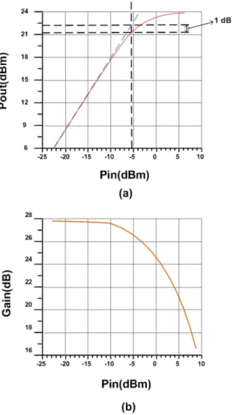
2.2 Power Amplifier Characteristics (a) Output Power (b) Gain . . . 3
2.3 IMD products due to AM/AM and AM/PM Conversion . . . 4
2.4 Harmonic Distortion for Two Tone Signal . . . 5
2.5 AM/AM Distortion of Power Amplifier using Saleh Model . . . . 7
2.6 AM/PM Distortion of Power Amplifier using Saleh Model . . . . 7
3.1 Basic Predistortion Scheme . . . 9
3.2 Basic Predistortion Architecture . . . 10
3.3 LUT-Based predistorter Scheme . . . 12
3.4 Polynomial predistorter Scheme . . . 14
4.1 New Predistortion Structure . . . 17
4.2 LUT Adressing with respect to the amplitude . . . 18
4.3 Look-Up-Table Structure . . . 19
4.4 Flow-Diagram of the Algorithm . . . 20 ix
LIST OF FIGURES x
4.5 Matched-Filter Usage . . . 22
4.6 Adaptation Scheme . . . 23
4.7 Vector Representation for Adaptation . . . 24
4.8 16-QAM Signal Generation for Simulation . . . 25
4.9 Scatter Plot of the Simulation Signal . . . 25
4.10 Power Spectrum of Incoming Signal,Vm . . . 26
4.11 Scatter Plot of Power Amplifier Output without using Predistor-tion . . . 27
4.12 Power Spectrum of Power Amplifier Output without using Predis-tortion . . . 27
4.13 Power Spectrum of Power Amplifier Output using Predistortion,Va 28 4.14 Scatter Plot of Power Amplifier Output using Predistortion,Va . . 29
4.15 Power Spectrum of Power Amplifier Output with and without us-ing Predistortion . . . 29
4.16 Amplitude of the LUT Coefficients . . . 30
4.17 Phase of the LUT Coefficients . . . 31
5.1 High Level Hardware Structure . . . 33
5.2 Adaptation of Predistorter IP Core - (a)Old design (b) New design 34 5.3 Low Level Hardware Structure . . . 36
5.4 Simulation Model for Experimental Setup . . . 38
LIST OF FIGURES xi
5.6 System for Calculation of LUT Coefficients . . . 40
5.7 Flow for Finding Response of the Power Amplifier . . . 40
5.8 Power Spectrum of Incoming Signal . . . 44
5.9 Power Spectrum of Filtered Signal . . . 45
5.10 Power Spectrum of PA Output Without Using Predistortion . . . 45
5.11 AM/AM response of the Power Amplifier . . . 46
5.12 AM/AM response of the Power Amplifier . . . 47
5.13 AM/AM response of the Predistorter . . . 47
5.14 AM/AM response of the Predistorter . . . 48
5.15 Power Spectrum of PA Output Using Predistortion . . . 48
5.16 Spectrum of PA Output Using Predistortion at Low Input Power 50 5.17 Spectrum of PA Output Using Predistortion at High Input Power 50 5.18 Predistortion with LUT size = 32 . . . 51
5.19 Predistortion with LUT size = 64 . . . 51
Chapter 1
INTRODUCTION
1.1
Background
Spectral efficiency is very important in today’s mobile telecommunication sys-tems. The power amplifier efficiency and linearity is a critical design issue. The nonlinear characteristics of power amplifier causes the power amplifier output to interfere with the adjacent channels and this interference has to be avoided in communication systems. The way to avoid this interference is either to reduce the power efficiency or to use linearization techniques.
Predistortion is a technique to compansate the nonlinear response of the power amplifier. The power amplifier distorts the signal and in order to have a linear replica of the input signal at the output of the power amplifier, the signal is distorted before being passed to the power amplifier. This distortion is done in such a way that it cancels with the distortion of the power amplifier. This is why the method is called predistortion. The predistorter models the inverse of the power amplifier. The power amplifier introduces both phase and amplitude nonlinearities and based on these phase and amplitude response of the power am-plifier, a predistorter is constructed that has also nonlinear phase and amplitude responses. It uses these nonlinear responses to cancel the nonlinearity effects of the power amplifier.
CHAPTER 1. INTRODUCTION 2
The predistortion can be applied in baseband to the transmitted signal before the upconversion and it can be applied in digital domain. The digital predistor-tion is a flexible design and it is easy to adapt the predistorpredistor-tion to communicapredistor-tion systems. FPGAs or DSPs can be used to implement digital predistortion. An-other issue with the digital predistortion is that it can be made adaptive to the variations of the power amplifier characteristics over time. This method is called as the Adapative Digital Predistortion and throughout this thesis the studies are done to build an adaptive digital predistorter scheme.
1.2
Thesis Objective and Outline
Throughout this thesis, the aim is to develop a new adaptive digital predistor-tion scheme. The proposed scheme is easy to be implemented in hardware and software. The effects of design parameters will be observed to find the optimal scheme. The outline of the thesis is as follows: Chapter 2 is an introduction about the nonlinearity concept and the characteristics of the power amplifier showing the baseband model used in simulations. Chapter 3 describes the basic predistor-tion schemes in today’s systems. Chapter 4 introduces a new look-up-table based adaptive predistortion scheme and the simulation results. Chapter 5 presents a new hardware implementable adaptive predistortion scheme with the hardware and software design. The design in this proposed scheme can be easily adapted to other systems. Chapter 6 gives the conclusion and presents possible future work.
Chapter 2
POWER AMPLIFIER AND
NONLINEARITY
2.1
Concept of Nonlinearity
Let us characterize a system by a block box with input x(t) and output y(t) as shown in Figure 2.1. In general, the system is said to be nonlinear if the output power is a nonlinear function of the input power
y(t) = N [x(t)] (2.1) where N is the nonlinear transfer function. If we expand the nonlinear function in simple Taylor series, the result shows the dependence of the nonlinearity on x(t)2. For periodic input signals, the nonlinearity results in the generation of
new frequency components at the output, as shown in Figure 2.1. This distortion caused by nonlinear systems is in the form of crossmodulation and intermodula-tion at the output signal spectrum. As the amplitude arises, these modulaintermodula-tion components grow faster than the signal itself and dominate the spectrum. This distortion cannot be prevented by using linear operations such as filtering since intermodulation causes new frequency components get bigger in the adjacent channels. As a result, the phase and the amplitude of the output signal will be affected depending on the amplitude and phase of the input signal. These effects
CHAPTER 2. POWER AMPLIFIER AND NONLINEARITY 2
lead to distortion at the output signal.
Figure 2.1: A Nonlinear System
2.2
Power Amplifier Characteristics
In telecommunications obtaining the output power high enough is the task of a power amplifier. After the modulation and upconversion, the input is multiplied with a gain by power amplifier to achieve the required power at the output. As it can be seen from the Figure 2.2(b) the gain is constant for low input powers and it reduces as approaching its saturation region. Saturation region is easily visible from the output power curve where inrease in input power brings no additional increase in output power. In Figure 2.2 (a) 1 dB compression point is also shown, which refers to the output power level at which the amplifier’s transfer characteristics deviates from the ideal one by 1 dB. This is a widely used measure of amplifier linearity.
Power amplifiers are mainly characterized by the second and third-order in-tercept point, 1 dB gain compression point and input back-off. When the input is increased, the second harmonic will increase proportional to the square of the input signal and the third harmonic will increase proportional to the cube of the input signal which means that the second and the third harmonics will increase at a greater rate than the fundamental component. The signal level at which the second harmonic is equal to the fundamental is called the second order intercept
CHAPTER 2. POWER AMPLIFIER AND NONLINEARITY 3
Figure 2.2: Power Amplifier Characteristics (a) Output Power (b) Gain point and the point at which the third harmonic is equal to the fundamental is called the third order intercept point. The 1 dB compression point is defined as the point at which the output power level has dropped 1 dB below the ideal output power. The ideal output power is the power where the power amplifier is fully linear. Input back-off is defined as the ratio of the signal power measured at the input of the power amplifier to the input signal power that produces the maximum signal power at the amplifier’s output.
CHAPTER 2. POWER AMPLIFIER AND NONLINEARITY 4
2.3
AM/AM and AM/PM Nonlinearity of
Power Amplifiers
Nonlinear relation between input and output power leads to AM/AM distortion. If the input signal includes amplitude modulation, power amplifier nonlinearity converts this modulation also into phase modulation and distorts the phase of the input signal. This is known as AM/PM conversion effect of the power amplifier. These two effects are shown in Figure 2.3.
Figure 2.3: IMD products due to AM/AM and AM/PM Conversion
A nonlinear and memoryless power amplifier can be modeled as a power series transfer function and the input-output relation of the power amplifier can be written as in Equation 2.2.
Vo(t) = a0+ a1Vin(t) + a2Vin(t)2+ a3Vin(t)3+ a4Vin(t)4+ a5Vin(t)5+ · · · (2.2)
A two-tone test signal can be applied to the input of the power amplifier whose relation is given by Equation 2.2. The two tone test signal is given in Eguation 2.3.
Vin(t) = vcos(w1t) + vcos(w2t) (2.3)
Then the output of the power amplifier is given by Equation 2.4 Vo(t) = a1v[cos(w1t) + cos(w2t)] + a2v2[cos(w1t) + cos(w2t)]2+
a3v3[cos(w1t) + cos(w2t)]3+ a4v4[cos(w1t) + cos(w2t)]4+
CHAPTER 2. POWER AMPLIFIER AND NONLINEARITY 5
The terms, except the fundamental term, in Equation 2.4 generates distor-tion products . In general, even order terms generate products which can be ac-cepted as out-of-band distortion. Out-of-band distortion products can be avoided by linear operations. However, odd order terms generate distortion products which are in-band and they are hard to get rid of. The adjacent band tortion is a very important problem in communications while out-of-band dis-tortion can be suppressed by filtering. In Figure 2.4, the fundamental
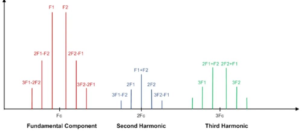
compo-Figure 2.4: Harmonic Distortion for Two Tone Signal
nent,second and third harmonic products are shown. Second and third harmonic products are far from the fundamental component and can be avoided. How-ever the distortion products which are adjacent to the fundamental component (2F 1 − F 2, 2F 2 − F 1, 3F 1 − 2F 2, 3F 2 − 2F 1) are difficult to be avoid. And also their amplitudes grow faster than the fundamental component’s amplitude and it becomes a problem if the power amplifier is to be operated at a high input power level.
2.4
Power Amplifier Modeling
The AM/AM and AM/PM distortion of the power amplifier can be modeled as a nonlinear complex gain. In the simulations throughout this thesis, the Saleh model for memoryless power amplifiers([1]) have been used. The model is con-structed in baseband as a complex baseband gain. It simply generates a complex
CHAPTER 2. POWER AMPLIFIER AND NONLINEARITY 6
gain whose phase and amplitude depend on the amplitude of the input signal. The distortion functions are given by Equations 2.5 and 2.6.
FAM/AM(r) = α 1 + βr2 (2.5) FAM/P M(r) = Ar2 1 + Br2 (2.6)
where α, β, A, B are constants which can be used to define the nonlinear char-acteristics of the power amplifier. In the simulations throughout this thesis they are selected as
α = 3 β = 0.0552 A = 1
B = 9 (2.7)
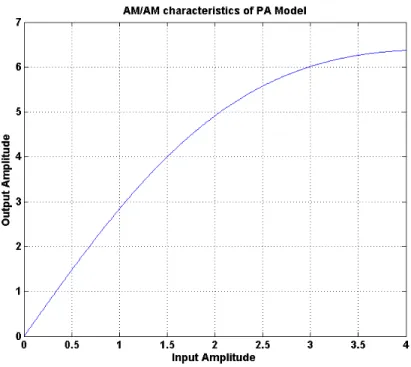
Using the values in Eguation 2.7 the power amplifier is modeled in baseband. The AM/AM and AM/PM distortion is plotted in Figures 2.5 and 2.6.
Let us assume a signal a + jb = rjθ in baseband is passing through the power
amplifier model. Depending on the amplitude of the input signal(r =√a2+ b2),
a complex gain is found using Equations 2.5 and 2.6. The complex gain has amplitude |G(r)| = FAM/AM(r) and phase6 G(r) = FAM/P M(r). Then the output
of the power amplifier model is calculated as the multiplication of two complex numbers : rejθ and |G(r)|ej6 G(r). The output is r|G(r)|ej(θ+6 G(r)) and it is not a linear function of the input signal.
CHAPTER 2. POWER AMPLIFIER AND NONLINEARITY 7
Figure 2.5: AM/AM Distortion of Power Amplifier using Saleh Model
Chapter 3
LINEARIZATION USING
PREDISTORTION
This chapter focuses on linearization of power amplifiers using adaptive digital predistortion showing some of the schemes using today : LUT-based predistortion and polynomial based predistortion.
3.1
Basics of Predistortion
Predistortion is a technique to obtain linear amplification and high power effi-ciency. It allows the power amplifier to operate at higher power level by correcting the distortion, caused by nonlinearity, up to the saturation. Beyond the satura-tion level the distorsatura-tion cannot be recovered since any increase in input power will generate no additional increase in output power.
The principle of the predistortion is to distort the signal in such a way that the cascade response of the predistorter and the power amplifier is linear. For this purpose, a nonlinear predistorter block is implemented in front of the power amplifier. The predistorter block then generates a distortion which compansates the distortion of the power amplifier and the output of the power amplifier has a
CHAPTER 3. LINEARIZATION USING PREDISTORTION 9
linear relation with the input of the predistorter.
Figure 3.1: Basic Predistortion Scheme
Referring to Figure 3.1, power amplifier output,Vo, is a scaled replica of the
predistorter input, Vi. Writing down the input-output relations for the blocks in
Figure 3.1 we get the following equations: Vp = ViF (|Vi|)
Vo = VpG(|Vp|) (3.1)
writing kVi for Vo and Vp = ViF (|Vi|) in the above equations we get Equation
3.2
kVi = G(|ViF (|Vi|)|)F (|Vi|)V i
k = G(|ViF (|Vi|)|)F (|Vi|) (3.2)
The equation 3.2 shows the condition for the predistorter to linearize the power amplifier. This equation is important in the sense that it tells us that, in order to linearize the power amplifier, we first have to know the response of the power amplifier which is the G(.) function in Equation 3.2. The performance of the linearization is directly depending on how precise we know or estimate the AM/AM and AM/PM response of the power amplifier. If the precision is poor, linearization will also be poor.
CHAPTER 3. LINEARIZATION USING PREDISTORTION 10
3.2
Digital Predistortion
Digital predistortion is implemented in baseband and this method is used in base-stations for mobile communication systems for linearity improvement, where adjacent channel power ratio is an issue. Digital predistortion is simple, stable and flexible. It can be adapted to the variations of the power amplifier and other circuit components. This adaptation capability is a powerful property in the expense of the hardware and software complexity. Figure 3.2 is the generic structure used for adaptive digital predistortion.
Figure 3.2: Basic Predistortion Architecture
Digital Predistorter techniques use the architecture in Figure 3.2. The sam-ples in baseband pass through the predistorter before being transmitted to the power amplifier and the output of the predistorter is sent to the D/A converter. Upconversion is then applied to the output of the D/A converter before the power amplifier. Power amplifier output is divided into two parts : one for trans-mission to antenna and one for feedback to the predistorter. The latter part is downconverted and then sampled by the A/D converter. The carrier of the downconversion and upconversion has to be common. The output samples of the A/D converter is fed into the predistorter for the adaptation operation. In gen-eral predistorter learns the characteristics(AM/AM and AM/PM responses of the power amplifier) using the feedback path. Predistorter knows the data it sends to the power amplifier and the data it receives from the power amplifier. Using this information, it adapts itself and distorts the samples in baseband to compansate the power amplifier distortion. Feedback path makes the predistorter technique a powerful technique in terms of adaptation capability. However, it also brings
CHAPTER 3. LINEARIZATION USING PREDISTORTION 11
stability problem and hardware and software complexity. Stability problem has to be taken into account and predistorter has to be prevented to go into unstable operation.
3.3
Digital Predistortion Schemes
There are mainly two different digital predistortion types : the LUT based predistorter([2],[3]) and the polynomial predistorter([4],[5]). In LUT-based pre-distortion, predistorter is modeled as a look-up table whose coefficients are com-plex values. Incoming signal is multiplied with the comcom-plex gain from the LUT according to its amplitude. In polynomial predistortion, predistorter is modeled as a polynomial function and the coefficients of the polynomial are adapted so that the predistorter and the power amplifier is linear. In theory, LUT-based predistorter can linearize the power amplifier more precisely while the precision of the polynomial predistortion directly depends on the order of the polynomial. In general 5thorder polynomial is required to suppress the 3rdand 5thorder IMD
products in the adjacent frequency band ([4]). In LUT-based method, the adap-tation is done by comparing the inphase and quadrature values of the incoming signal and the output of the power amplifier. The input of the predistorter is the original signal and adaptation is done to achieve the output of the power amplifier as a linear replica of the original signal. In polynomial predistortion, the adaptation is done to minimize the adjacent channel power at the output of the power amplifier. This power is taken as an error signal and is to be minimized by polynomial predistortion using direct search or gradient methods. Adaptation algorithm, in terms of complexity, is difficult using polynomial predistortion.
CHAPTER 3. LINEARIZATION USING PREDISTORTION 12
3.3.1
Look-up-table (LUT) Based Predistortion
LUT-based predistorter is simpler than the polynomial predistorter if we consider the complexity and calculations. Only six multiplications are required while cal-culating the adress of the LUT and complex output signal. However, in polyno-mial predistortion, more multiplication and addition operations are required.
LUT coefficients must be calculated according to a particular addressing. Ad-dressing by the magnitude square is the easiest method and it can be done by simply adding the squares of the I and Q values of the input baseband signal. This is the power of the input signal. Addressing in this way gives more impor-tant to the power levels near saturation and it improves the efficiency and the linearization performance of the predistorter.
Figure 3.3: LUT-Based predistorter Scheme
A detailed block diagram of LUT-based predistorter is shown in Figure 3.3. The system including the predistorter consists of address calculation unit,LUT, complex multiplier, ADC, DAC, filters, modulator, demodulator, which has to have a common carrier with the modulator, and power amplifier. I and Q base-band signals are input to the system and they are multiplied by a complex gain from the LUT which models the inverse of the power amplifier characteristics. Once the complex signal Vi(t) arrives at the input, the address is obtained by
calculating the magnitude square and this address is sent to the LUT. Then the corresponding complex gain in the LUT is multiplied with the input signal and we get Vd(t). Vd(t) is then converted to the analog signal and after being filtered and
CHAPTER 3. LINEARIZATION USING PREDISTORTION 13
Vo(t) is used for adaptation to the variations of the characteristics of the power
amplifier for reliable operation.
Feedback signal Vf(t) and the original signal Vi(t) is used the find the error
signal and using the error signal the LUT coefficients are updated to have a linear relation between Vo(t) and Vi(t). In order to adapt the predistorter to
power amplifier nonlinearity variations Equation 3.2 can be used to update the LUT coefficients. In LUT-based method this equation is used to generate an iterative method which is in general the well-known LMS algorithm.
Referring to Figure 3.3, Let the predistorter response be F (.) and the power amplifier response be G(.). Then using Equation 3.2 the relationship between F (.) and G(.) for a linear response can be written as in Equation 3.3
K = F (xi)G(xi|F (xi)|) (3.3)
where xi is the amplitude of the incomig signal Vi. Then the adaptation is done
according to the Equation 3.4 as follows F (xi, j + 1) =
K G(xi|F (xi, j)|)
(3.4) In Equation 3.4, j is the iteration index and F (xi, j) is the complex LUT value
at iteration j. This equation can be solved by using LMS algorithm ([6]) and ap-plying this equation in runtime makes the predistortion adaptive. The variations in G(.) which are the variations of the characteristics of the power amplifier, will be adapted by changing the predistorter characteristics F (.) so that Equation 3.4 is satisfied.
3.3.2
Polynomial Predistortion
Polynomial predistorter uses complex polynomial function to model the inverse of the power amplifier. Each sample coming into the predistorter is processed using the ploynomial function. The order of the polynomial function depends on the distortion of the power amplifier. For instance, if power amplifier generates 5th order distortion products then a 5th order polynomial can be used. ([4],[5])
CHAPTER 3. LINEARIZATION USING PREDISTORTION 14
Figure 3.4 shows the detailed block diagram of a polynomial predistorter. The adaptation is done by updating the complex-valued coefficients of the polynomial function to fit the predistorter response to the inverse of the power amplifier.
The polynomial predistorter is composed of a address calculation unit using amplitude square as in LUT-based method, a polynomial predistortion function, a complex multiplier, an optimization circuit for polynomial coefficients, DAC, ADC and the feedback path. The number of multiplication and addition opera-tions is higher and it also arises with the order of the polynomial. The complex voltages V i(t), V d(t), V q(t) and V o(t) are as defined before in the LUT based predistorter case. Just the feedback signal Vf(t) is no more a complex voltage but
a scalar value proportional to the unwanted adjacent channel power emission. In the following the derivation of a polynomial predistortion system is given which is done according to magnitude square of the input.
Figure 3.4: Polynomial predistorter Scheme
The following analysis of the polynomial predistorter assumes the power am-plifier and predistorter response as a function of the magnitude square of the input signal. The odd powers of the magnitude are not used while modeling power amplifiers, because these terms do not generate in-band distortion prod-ucts. The referring to Figure 3.4, we can write the response of the power amplifier as
G(|Vd(t)|2) = β1+ β3|Vd(t)|2+ β5|Vd(t)|4 (3.5)
then the output of the power amplifier is written as
CHAPTER 3. LINEARIZATION USING PREDISTORTION 15
combining equations 3.5 and 3.6
Vo(t) = β1Vd(t) + β3Vd(t)|Vd(t)|2+ β5Vd(t)|Vd(t)|4 (3.7)
Like power amplifier, the predistorter is modeled as a function of the magni-tude square of the input signal as
F (|Vi(t)|2) = α1+ α3|Vi(t)|2+ α5|Vi(t)|4 (3.8)
the output of the power amplifier is written as
Vd(t) = Vi(t)F (|Vi(t)|2) (3.9)
From Equations 3.6 and 3.9 we can write the relationship between Vi(t) and Vo(t)
as
Vo(t) = Vi(t)F (|Vi(t)|2)G(|Vi(t)F (|Vi(t)|2)|2) (3.10)
and if the linear gain we are targeting to achieve is K then Equation 3.11 has to be satisfied.
Vo(t) = K(Vi(t))Vi(t) (3.11)
Using Equations 3.11 and 3.10 we can write
K(Vi(t)) = F (|Vi(t)|2)G(|Vi(t)F (|Vi(t)|2)|2) (3.12)
then K(Vi(t)) is a function of the magnitude square of Vi(t) and can be written
as
K(Vi(t)) = γ1+ γ3|Vi(t)|2 + γ5|Vi(t)|4 (3.13)
In order to liearize the power amplifier γ1 must be equal to the targeted gain
and γ3,γ5 must be small. Polynomial predistortion algorithms tries to achieve
Chapter 4
A NEW DIGITAL ADAPTIVE
PREDISTORTION METHOD
This chapter introduces a new algorithm for adaptive digital predistortion using look-up-table method. The following sections describe the new algorithm and show the simulation results. The algorithm works in baseband and throughout this chapter, power amplifier and predistorter will be modeled as they both work in baseband. For power amplifier baseband model, we will use the nonlinear memoryless Saleh model which is explained in Section 2.4
4.1
New predistorter Scheme
The scheme to be used in the adaptive digital predistorter is given in Figure 4.1. It consists of complex multiplier, delay elements, LUT, adaptation logic and power amplifier.
The LUT and complex multiplier models the predistorter response and the adaptation logic updates the coefficients of the LUT according to the power am-plifier characteristics. The coefficients of the LUT are complex. These complex coefficients are calculated by the adaptation logic. The blocks in Figure 4.1 is
CHAPTER 4. A NEW DIGITAL ADAPTIVE PREDISTORTION METHOD 17
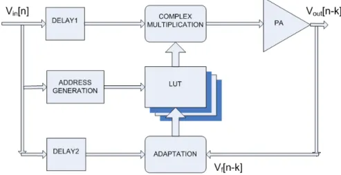
Figure 4.1: New Predistortion Structure explained in detail in the following subsections.
4.1.1
Delay Elements
The delay elements in the adaptive predistorter scheme provide alignment. There are two delay elements in Figure 4.1. The first one, DELAY1, is used in order to align the data with its corresponding LUT coefficients. If the latency caused by address generation from the input signal is t1 and the latency caused the loading
of the corresponding complex coefficient to the complex multiplier is t2, then in
order to multiply the input signal with its corresponding complex LUT value, we have to have a delay of t1+ t2. This delay is DELAY1. DELAY2 is required to
align the incoming data,Vin[n] and the feedback data,Vf[n − k]. The adaptation
logic has to know the feedback data corresponding to the incoming data and DELAY2 is used for this purpose. One of the key points in this design is that the DELAY2 resolution depend directly on the sampling rate. For instance, if the sampling clock period is 10ns(nanoseconds), and the delay between incoming data and the feedback data is 55ns, then the latency is assumed as 50ns or 60ns. This is expected since the alignment is done in discrete time domain and the resolution is limited with the sampling period.
CHAPTER 4. A NEW DIGITAL ADAPTIVE PREDISTORTION METHOD 18
4.1.2
Address Calculation
The LUT is addressed according to the magnitude square of the input baseband signal. The address calculation unit simply finds the amplitude square of a com-plex number. It maps the amplitude square of the input signal to the address of the LUT. This mapping with amplitude square enables giving more importance to the high amplitude signals where the power amplifier is nonlinear, and giving less importance to low amplitude signals where the power amplifier is linear. The
Figure 4.2: LUT Adressing with respect to the amplitude
Figure 4.2 shows the LUT address with respect to the amplitude if the LUT ad-dress is linear with amplitude square of the signal. With the same interval on the amplitude axis, we have more address space at high amplitudes. R1 is the address
range for input amplitudes between 4 and 6 and R2 is the address range for input
amplitudes between 8 and 10 and it is clear that R2 > R1 which means that we
CHAPTER 4. A NEW DIGITAL ADAPTIVE PREDISTORTION METHOD 19
4.1.3
Complex Multiplication
In order to compansate both AM/AM and AM/PM distortions of the power amplifier the LUT coeeficients are chosen to be complex. The complex multi-plier multiplies the input sample with its corresponding complex gain. Complex multiplication means that we are changing the amplitude and the phase of the incoming sample.
4.1.4
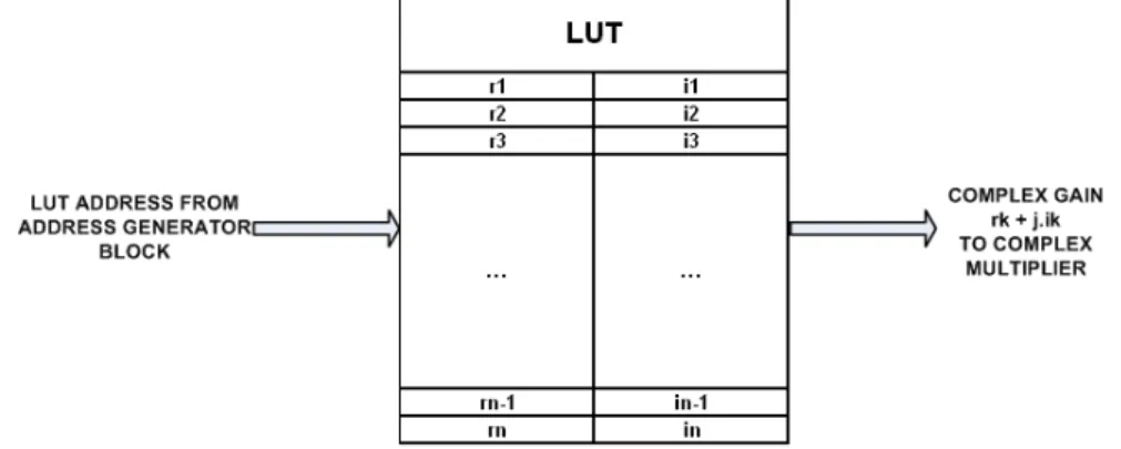
Look-Up-Table
Look up table is one of the core blocks of the predistorter and it models the inverse of the power amplifier. The structure of the LUT is shown in Figure 4.3. The LUT which is used in this algorithm has two parts : real part and imaginary part. For every incoming sample, LUT is addressed and a complex gain rk+ jik
Figure 4.3: Look-Up-Table Structure
is loaded to the complex multiplier. This complex gain is multiplied with the incoming baseband signal and compansates it for phase and amplitude distortion of the power amplifier.
4.1.5
Adaptation
The adaptation logic is a block which inputs incoming samples and feedback samples and outputs LUT coefficients. The difference of the new algorithm from
CHAPTER 4. A NEW DIGITAL ADAPTIVE PREDISTORTION METHOD 20
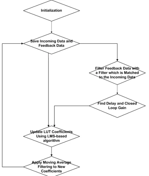
other LUT-based methods is based on the difference of the adaptation of the LUT to the variations of the power amplifier. The new proposed method is summarized in Figure 4.4. The steps of the flowchart is explained in this section in detail.
Figure 4.4: Flow-Diagram of the Algorithm
4.1.5.1 Initialization
In this step, we initialize all the LUT coefficients for unit delay. For this purpose we set all the real parts of the LUT coefficients to 1 and all the imaginary parts
CHAPTER 4. A NEW DIGITAL ADAPTIVE PREDISTORTION METHOD 21
of the LUT coefficients to 0.
4.1.5.2 Finding Delay and Closed-Loop Gain
The delay between incoming data and the feedback data has to be known for alignment. The gain of the closed loop also has to be known for the adaptation algorithm. In order to find these variables, a matched filter is used. This filter is matched filter of the incoming data and it is applied to the feedback data. The filtering operation is shown in the following Equations :
s0[n] = as[n − k] + v[n] (4.1) where s0[n] is the feedback data, s[n] is the incoming data, a is the closed-loop gain,k is the delay between incoming data and feedback data and v[n] is the noise which is assumed to be independent of feedback data and incoming data. Then Using Equation 4.1 we can write Equation 4.2
< s0[n], s[n] > ||s[n]||2 = < as[n − k] + v[n], s[n] > ||s[n]||2 = < as[n − k], s[n] > ||s[n]||2 + < v[n], s[n] > ||s[n]||2 (4.2)
The < . > operation in Equation 4.2 is the inner product operation. Notice that the second term in this Equation is zero since the noise is independent of the incoming data. So the result is simply the inner product of the incoming data with itself at lag k multiplied by the closed-loop gain and divided by the norm-square of the incoming data as in Equation 4.3
< s0[n], s[n − l] > ||s[n − l]||2 = a
< s[n − k], s[n − l] >
||s[n − l]||2 (4.3)
Equation 4.3 shows us the way to find the delay and closed-loop gain. The term in this equation gives its maximum when l = k. The result at lag k is simply the closed-loop gain since < s[n − k], s[n − k] > is equal to ||s[n − k]||2. So in order
to find the delay we have to find at which lag < s0[n], s[n − l] > is maximum and the a parameter at this lag gives us the closed-loop gain. The method to find gain and delay variables is shown in Equations 4.4 and 4.5.
gain = max
l
< s0[n], s[n − l] >
CHAPTER 4. A NEW DIGITAL ADAPTIVE PREDISTORTION METHOD 22
delay = arg max
l
< s0[n], s[n − l] >
||s[n]||2 (4.5)
The Equations 4.4 and 4.5 can be implemented using a filter which is matched to the incoming data,s[n]. So the impulse response of the filter is sM F[n] = s∗[−n]
and y[n],the output of the convolution of the feedback data with the matched filter sM F[n], is shown in Equation 4.6.
y[l] =
∞
X
k=−∞
s0[k]sM F[l − k] (4.6)
Substituting sM F[n] = s∗[−n] into Equation 4.6 we get Equation 4.7.
y[l] =
∞
X
k=−∞
s0[k]s∗[k − l] =< s0[n], s[n − l] > (4.7) We find a scheme to implement Equation 4.7 as in Figure 4.5. The normalization simply divides y[n] to the norm-square term,||s[n]||2
Figure 4.5: Matched-Filter Usage
4.1.5.3 Coefficient Update Algorithm
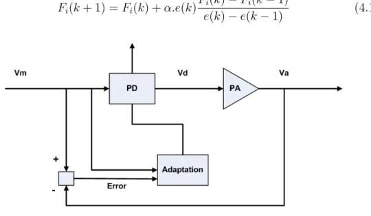
Before developping our own method, we used secant method for updating the LUT coefficients([6]). Referencing the Figure 4.6 the following steps were followed in order to apply the secant method.
Step1 : Find the index for the input signal V m(k). Indexing of the LUT was done with respect to the amplitude-square of the input samples. Let this index be i.
Step2 : Multiply the input sample with the corresponding gain of the predistorter,F i(k)).
CHAPTER 4. A NEW DIGITAL ADAPTIVE PREDISTORTION METHOD 23
Step3 : Find the error signal
e(k) = P AGain.V m(k) − V a(k) (4.9)
Step4 : Update the gain at the index i of the LUT using secant method Fi(k + 1) = Fi(k) + α.e(k)
Fi(k) − Fi(k − 1)
e(k) − e(k − 1) (4.10)
Figure 4.6: Adaptation Scheme
Following these steps, we try to find an easier way to update the LUT coeffi-cients. In other words, we try to change this algorithm in Step4 to have an easier and hardware implementable method. In real life while implementing this design on FPGA, the division operation in the algorithm takes too many resources and the design is not cost-effective. For that reason we had to add some improvement to the algorithm and in other words we have to find a term instead of the frac-tional term. The new term is found by observing Step4 in vector domain. The vector representation of the new method is shown in Figure 4.7-a. The vectoral representation shows the baseband signals in two dimensional vector domain. The error signal is shown in Figure 4.7-a. Our aim for linearization is to move the output of the power amplifier,Va[k], towards the input of the predistorter,Vm[k],
assuming the power amplifier has unity gain in linear region. In order to have undistorted sample at the output of the power amplifier, we have to rotate the incoming sample, in other words the gain of the predistorter must move Vm(k) in
the direction so that Va(k) moves towards Vm(k). This means that we must
CHAPTER 4. A NEW DIGITAL ADAPTIVE PREDISTORTION METHOD 24
Figure 4.7: Vector Representation for Adaptation
Vm(k) in the desired direction. A suitable term is −(V m∗). The explanation of
multiplication with −(V m∗) is shown in Figure 4.7-b. We know that when we multiply two complex numbers we add their angles and multiply their amplitudes. And in order to move Va[k] towards Vm[k], the predistorter must multiply Vm[k]
with a complex number such that Vm[k] and Va[k] move in the direction shown in
Figure 4.7-b. In this method, convergence is an issue and α parameter has to be chosen properly so that the update algorithm is stable and convergent. Choosing small α increases the convergence time while it makes the method more stable.
4.1.6
Moving-Average Filtering to LUT coefficients
After updating the LUT coefficients, MA filtering is applied. In simulations a 9-tap MA filter is used. The impulse response of the filter is given in Equation 4.11. h[n] = 4 X k=−4 1 9δ[n − k] (4.11) This filtering is done to improve convergence time. It sets the neighboring LUT cells even if there has been no sample corresponding to those cells.
CHAPTER 4. A NEW DIGITAL ADAPTIVE PREDISTORTION METHOD 25
4.2
Simulations and Results
We begin simulations by first generating a 16-QAM signal in baseband as shown in Figure 4.8. In this Figure there are 3 blocks used to generate the simulation signal. The first block is Random Integer Generator generates integer from 0 to 15 and Rectangular QAM modulator maps this integer value to a complex number which is included in the constellation of the 16-QAM modulation. The output of the QAM modulator is passed through a pulse shaping filter and the output of the pulse shaping filter is the signal which is used in our simulations.
Figure 4.8: 16-QAM Signal Generation for Simulation
Figure 4.9: Scatter Plot of the Simulation Signal
CHAPTER 4. A NEW DIGITAL ADAPTIVE PREDISTORTION METHOD 26
spectrum of the generated signal is given in Figure 4.10. The constellation of 16-QAM modulation is clearly seen in the scatter plot.
Figure 4.10: Power Spectrum of Incoming Signal,Vm
The generated signal is the input signal of the predistorter which corresponds to Vm in Figure 4.6. Before simulating the predistorter, the input signal is first
passed through the power amplifier without predistortion to see the effects of the power amplifier nonlinearity on the scatter plot and the power spectrum of the output signal. The scatter plot is shown in Figure 4.11. This scatter plot shows the effect of the nonlinearity on the 16-QAM constellation. The constellation is rotated by the power amplifier. In addition, the power spectrum of the output signal is shown in Figure 4.12. The power amplifier amplifies the signal however, the distortion occurs in adjacent frequency bands. This distortion is caused by the third order nonlinearity of the power amplifier so that ACPR is 20dB worse than the incoming signal. The rotation of the constellation in the scatter plot and the distortion of the power spectrum is caused by the AM/AM and AM/PM nonlinearities of the power amplifier model used in the simulations.
CHAPTER 4. A NEW DIGITAL ADAPTIVE PREDISTORTION METHOD 27
Figure 4.11: Scatter Plot of Power Amplifier Output without using Predistortion
Figure 4.12: Power Spectrum of Power Amplifier Output without using Predis-tortion
CHAPTER 4. A NEW DIGITAL ADAPTIVE PREDISTORTION METHOD 28
After observing the effects of the power amplifier on the input signal, the predistorter is used to see if it compansates the nonlinearity caused by the power amplifier. In this case we used the scheme which is explained in Section 4.1.The input signal is passed through the predistorter before passing through the power amplifier. The scatter plot and power spectrum of the output signal is shown in Figure 4.14 and Figure 4.13 respectively. The scatter plot shows that predis-torter compansates the rotation of the constellation and the output constellation seems to be an amplified replica of the input constellation. The power spectrum shows that the third order distortion is compansated so that ACPR is improved by nearly 20 dB. The power spectrum plot in Figure 4.15 shows the improvement in ACPR more clearly by plotting the output spectrum of the power amplifier with and without using predistortion. The 20dB improvement in ACPR is shown in this figure. The compensation of the constellation and power spectrum means that the predistorter linearizes the power amplifier as expected.
CHAPTER 4. A NEW DIGITAL ADAPTIVE PREDISTORTION METHOD 29
Figure 4.14: Scatter Plot of Power Amplifier Output using Predistortion,Va
Figure 4.15: Power Spectrum of Power Amplifier Output with and without using Predistortion
CHAPTER 4. A NEW DIGITAL ADAPTIVE PREDISTORTION METHOD 30
In addition to observing the power spectrum and scatter plots for the predis-torter signal, the LUT coefficients are observed to see their amplitudes and phase when the algorithm has converged. The amplitude of the LUT coeeficient with respect to LUT index is shown in Figure 4.16 and the phase is shown in Figure 4.17. The amplitude of the LUT coefficients is like a monotonically increasing function. The high amplitude input signals have to be amplified more by the predistorter since the gain of the power amplifier for high amplitude signals is less. So the resulting plot of the amplitude of the LUT coefficients is an expected plot. The Phase of the LUT coefficients is like a monotonically decreasing func-tion with respect to LUT index. If we observe the AM/PM response of the power amplifier model which is given in Figure 2.6, in order to compansate the phase distortion we have to add the inverse of the hase of the power amplifier to the input signal and the plot of phase of LUT coefficients is an expected plot which compansates the phase gain and makes the cascaded system(predistorter+power amplifier) have linear phase.
Figure 4.16: Amplitude of the LUT Coefficients
We notice that the very high indexes of the LUT is not calculated by the adaptation algorithm. The reason is the amplitude of the input signal is not so high to address the high indexes of the LUT.
CHAPTER 4. A NEW DIGITAL ADAPTIVE PREDISTORTION METHOD 31
Figure 4.17: Phase of the LUT Coefficients
This New Digital Adaptive Predistortion Method has been simulated in MAT-LAB but it has not been verified in hardware. The simulations show us that the LUT coefficients converge after processing 1 Mega samples. It is not practical to use this type of algorithm in the software of a processor and this algorithm has to be done purely in hardware for convergence issue. Next chapter explains an easy hardware implementable adaptive predistortion scheme where a processor is used.
Chapter 5
HARDWARE
IMPLEMENTABLE
PREDISTORTER
In the previous chapter, we proposed a new LUT-based adaptive digital predistor-tion scheme. This new scheme can be used as a hardware block in communicapredistor-tion systems. However, if we have a processor in our hardware design then the adap-tation of the predistortion can be done by the software of the processor. Using this technique, no hardware resources will be used for adaptation.In addition, predistorter design with processor is more flexible and easily adaptable to other systems.
This chapter focuses on an easy hardware implementable adaptive predistor-tion scheme. For this purpose an IP Core in hdl(Hardware Descrippredistor-tion Language) is designed and implemented in hardware. The steps in the design of the predis-torter are explained in detail.
CHAPTER 5. HARDWARE IMPLEMENTABLE PREDISTORTER 33
5.1
Hardware Implementation of Predistorter
In order to realize the predistortion, the hardware implementation is necessary and we should find an effective way of implementation. The method we use is to design an IP Core in FPGA and connect it to the hard processor which will control the IP Core. The high level structure of the hardware design is shown in Figure 5.1. As we see in this Figure, the IP inputs the incoming baseband signal and the feedback IF signal and it outputs the baseband signal to be upconverted for transmission to power amplifier. The controls of the IP Core is done by the processor via the processor local bus. The IP Core has an interface with this local bus for the transaction of control and data signals between processor and the predistorter.([7])The idea to apply predistortion is to get a predetermined number of samples from incoming signal and feedback signal and then send this samples to processor via the local bus. The processor will run the predistortion algorithm and load the LUT coefficients back to the IP via the local bus. This method is an offline predistorion method but it is still adaptive. The predistortion is done in software of the processor and this makes the predistortion flexible and easily adaptable to other systems. Any predistortion scheme which uses LUT-based method can use this hardware. Since the only change in different LUT-based predistortion is the adaptation part and it is done in software for this design, the hardware for all these different predistorter methods will be the same.
CHAPTER 5. HARDWARE IMPLEMENTABLE PREDISTORTER 34
The hardware system in Figure5.1 is designed as a generic IP Core for adap-tation to all LUT-based memoryless predistortion systems. The only thing to be done to adapt this generic hardware is putting this IP Core before the upcon-version. The baseband signals which were sent to the upconverter will be first passed through the IP Core and the outputs of the IP will be connected to the input of the upconverter. The Figure 5.2 shows the basic structure to connect the IP Core to any design which uses LUT-based method. If the system in Figure 5.2-a is to be adapted for using predistortion, the system in Figure 5.2-b can be used to adapt out IP Core to the system.
Figure 5.2: Adaptation of Predistorter IP Core - (a)Old design (b) New design The low level hardware implementation of the predistorter and the internal hardware structure is shown in Figure 5.3. The hardware is implemented in FPGA(Virtex4-fx100) which has hard PowerPC processor core and the Figure 5.3 shows the controls of the IP Core by the PowerPC. The predistorter can be seperated into 3 subblocks and the function of each subblock is explained in the following sections.
5.1.1
Subblock1 : Predistortion
This subblock of the predistorter block includes the Address Calculation, LUT, Delay and Complex Multiplier. The Address Calculation is done by adding the
CHAPTER 5. HARDWARE IMPLEMENTABLE PREDISTORTER 35
squares of the inphase and quadrature components of the incoming baseband sig-nal. The address, generated by this block is sent to LUT to get the corresponding complex gain. Then the delayed baseband signal is multiplied by the LUT com-plex gain and this subblock outputs the predistorted signal. The LUT in this subblock can be updated by the PowerPC and for this reason the write port of the LUT is connected to local bus of the processor. The adaptation software will update the LUT via this write port. This subblock works real-time. For every incoming sample the Address calculation, LUT addressing, Delay element and Complex Multiplier are used to generate the corresponding baseband sample, in other words this subblock works continuously.
5.1.2
Subblock2 : Adaptation Hardware
Subblock2 in Figure 5.3, functions as a memory which samples the feedback base-band signal and the incoming basebase-band signal. The feedback IF signal is down-converted usind the Direct Digital Synthesizer block. The DDS (Direct Digital Synthesizer) is used to generate the sine and cosine for the IF downconversion. The output frequency of the DDS is software controllable and can be adjusted by the PowerPC according to the center frequency of the feedback IF signal.
There are two memories to save the baseband samples from the incoming signal and the feedback signal. These are Input Sample Memory and Feedback Sample Memory, respectively. The write ports of these memories are connected to the internal hardware and the read ports are connected to PowerPC. PowerPC can read the baseband samples from both memories and updates the LUT coefficients according to these samples. This subblock is used for Adaptation and it does not work continuously. The sampling operation starts with a command given by PowerPC. When the sampling command arrives, this subblock samples 4K(4096) baseband samples and waits for PowerPC to read the memories. After PowerPC reads these memories, it runs the predistortion algorithm and updates the LUT. The next command for sampling has to be started after a certain amount of time because the updated LUT will effect the output of the power amplifier after some time. So the software algorithm has to wait before sampling the baseband
CHAPTER 5. HARDWARE IMPLEMENTABLE PREDISTORTER 36
Figure 5.3: Low Level Hardware Structure samples again.
5.1.3
Subblock3 : Hardware Simulation
Subblock3 in Figure 5.3, is used for simulation purpose. At the output stage of the predistorter, a nonlinearity model is designed and the nonlinear characteristics of this model can be determined by PowerPC. In our experiments we started our simulations by first generating a nonlinear model in hardware and connect the output of the DAC to input of the ADC. Using this loopback operation and generating the nonlinearity model in hardware we modeled the power amplifier characteristics without using the power amplifier and the RF circuits. This is
CHAPTER 5. HARDWARE IMPLEMENTABLE PREDISTORTER 37
a way of simulating our predistortion algorithm in hardware. The nonlinearity model can be disabled or enabled by PowerPC by the control of the multiplexer in the output stage. For instance, the Nonlinearity model is adjusted to give third order distortion by setting its AM gain as a function of the square of index. Then the predistortion algorithm runs in software and the output of the DAC is observed to be linear replica of the input of the predistorter. The nonlinearity model consists of an Address Calculator, a LUT and a Complex Multiplier as in subblock2. The address of the nonlinear LUT is calculated by the address calculator and the output of the LUT is multiplied by the baseband signal. This is the same operation used in subblock2.
5.2
Software Development for Predistortion
After designing a generic hardware in Section 5.1, we have the opportunity of working with real data. The first thing we do is to get real samples from incoming baseband signal and process it in MATLAB using the power amplifier simulation model. The second step is to get real samples from incoming baseband signal and the feedback baseband signal and process it in MATLAB. The second step continues with writing the LUT in the hardware with tha data which is found in MATLAB software offline. The last step is to do all the software in PowerPC software. These three steps will be explained in detail in the following subsections.
5.2.1
Software Development Step1 : MATLAB
Simula-tion with Real Data
The simulation of the experimental setup is very crucial step in our study. The setup is shown in Figure 5.4. The model consists of a predistorter, a low-pass filter and the power amplifier. The filter is modeling the band-pass filter infront of the power amplifier. Since we run our simulations in baseband, the band-pass filter is modeled as a low-pass filter considering the bandwidth of the band-pass filter.
CHAPTER 5. HARDWARE IMPLEMENTABLE PREDISTORTER 38
Figure 5.4: Simulation Model for Experimental Setup
The flow of the simulation is shown in flow chart in Figure 5.5.The states are numbered in the flowchart in Figure 5.5. The flow starts by State0 and in this state the LUT of the predistorter is initialized for unity gain. Initially, no nonlinearity is introduced by the predistorter. So after the flow starts, initial state sets the LUT of the predistorter to all ones. In State1, the data is passed through the predistorter but after initialization the predistorter input and output is the same. So for the first time that we arrive State1, the predistorter equates its output to its input. In State2, the output of the predistorter is filtered by the low pass filter. The filtered signal is then passed through the power amplifier, which is modeled using Saleh model, which we have used in all our simulations throughout this thesis. In State4 the LUT coefficients of the predistorter are calculated using the incoming and feedback baseband signals. In State5 the LUT of the predistorter is loaded with the calculated coefficients and then we return back to State1. For this turn, predistorter no longer has unity gain and it introduces nonlinearity to compansate the nonlinearity of the power amplifier. The states are then followed according to the flow in Figure 5.5. The key step in the flow is to calculate the coefficients of the LUT of the predistorter. The method that we used for the calculation is a new method and it is introduced in this subsection.
5.2.1.1 Calculation of the LUT Coefficients
Based on the Scheme in Figure 5.7, we derive an algorithm for calculation of the LUT coefficients. The flow of the algorithm is shown in Figure 5.7. The first step is the alignment of the incoming and the feedback data. The alignment is done by the method explained in section 4.1.5.2. In addition to the alignment in
CHAPTER 5. HARDWARE IMPLEMENTABLE PREDISTORTER 39
Figure 5.5: Flow for Simulation of the Experimantal Setup
this section, the analog delay alignment is also done by using the phase of the output of the matched filter and this phase information is used for the alignment of the inphase and quadrature components of the incoming and feedback signals. After aligning tha data, next step is to find the AM/AM and AM/PM responses of the power amplifier. This is done by simply dividing the baseband feedback signal to the incoming baseband signal. In other words we divide two complex numbers.The output of the complex division gives the response of the power amplifier in baseband. The equation 5.1 shows the division operation.
Iin+ jQin
If eedback + jQf eedback
= |A|ejφ (5.1) According to the Equation 5.1, |A| is the amplitude of the division and φ is the phase of the division. The next step is to use this division result in finding the AM/AMand AM/PM responses of the power amplifier. As expected |A| values of each division is arranged with respect to the amplitude-square of the incoming
CHAPTER 5. HARDWARE IMPLEMENTABLE PREDISTORTER 40
Figure 5.6: System for Calculation of LUT Coefficients
signal and for the same amplitude-square address the arranged |A| values are averaged to get the AM/AM response of the power amplifier corresponding to that amplitude-squared address. The AM/PM response is also found by the same way and this time φ parameters of the divisions are used. The figure 5.7 shows the calculation operation step-by-step.
Figure 5.7: Flow for Finding Response of the Power Amplifier
After finding the response of the power amplifier, the next step is to find the coefficients for the predistorter. The following iterative steps shows the way which we used to find the LUT coefficients referring to Figure 5.6:
Step0 : Initialize f (.) for unity gain for all inputs. To do this, set the complex values of the LUT of the predistorter to 1 + j0. This operation equates Vpd to
CHAPTER 5. HARDWARE IMPLEMENTABLE PREDISTORTER 41
Vin.
Then find g0(.) by the following equations :
Vpa = Vpd.g0(|Vpd|2) (5.2)
g0(|Vin|2) =
Vpa
Vpa
(5.3)
After finding g0(.), find f0(.) that makes Vpa = Vin using the following
equa-tions :
Vpd = Vin.f0(|Vin|2) (5.4)
Vpa = Vpd.g0(|Vpd|2) = Vin.f0(|Vin|2).g0(|Vin|2.|f0(|Vin|2)|2) (5.5)
f0(|Vin|2).g0(|Vin|2.|f0(|Vin|2)|2) = 1 (5.6)
Putting k = |Vin|2 in Equation 5.6 we get :
f0(k).g0(k.|f0(k)|2) = 1 (5.7)
And knowing g0(.) function in 5.7, we find the predistorter function f0(.).
The problem of calculation of LUT coefficient reduces to finding the inverse of a function to find the predistorter LUT coefficients. The solution to this reduced problem is solved by an easy method which is found by Oguzhan Atak. He gives the name ”pred” to this method and the method will be explained in detail.
Step1 : Put f0(.) to the LUT of the predistroter and collect new samples
from the incoming and feedback signals.
Then find g1(.) by the following equations :
Vpd = Vin.f0(|Vin|2) (5.8) Vpa = Vpd.g1(|Vpd|2) (5.9) g1(|Vpd|2) = Vpa Vpd (5.10)
CHAPTER 5. HARDWARE IMPLEMENTABLE PREDISTORTER 42
After finding g1(.), find f1(.) that makes Vpa = Vin using the following
equa-tions :
f1(k).g1(k.|f1(k)|2) = 1 (5.11)
f1(.) is found by the method in Step0. The pred method is used in all steps
to find the LUT coefficients with known power amplifier response. .
. .
Stepi : Put fi−1(.) to the LUT of the predistroter and collect new samples
from the incoming and feedback signals.
Then find g1(.) by the following equations :
Vpd= Vin.fi−1(|Vin|2) (5.12) Vpa = Vpd.gi(|Vpd|2) (5.13) gi(|Vpd|2) = Vpa Vpd (5.14)
After finding gi(.), find fi(.) that makes Vpa= Vinusing the following equations
:
fi(k).gi(k.|fi(k)|2) = 1 (5.15)
The ”pred” method is explained in this part of this section. The ”pred” method is an easy and practical method to solve the equation f (k).g(k.|f (k)|2) =
1. It also uses the fact that the amplitude of g(k) function is a monotonically decreasing function. The method can be shown by the following states :
State0 : Assign f (k) to g(k)1 for all indexes. Set the initial index to zero, i=0. go to State1
CHAPTER 5. HARDWARE IMPLEMENTABLE PREDISTORTER 43
State2 : Calculate result = f (j).g(j.|f (j)|2). if result < 1 then go to State3
else go to State4
State3 : Decrease j. Assign f (j) = to g(j)1 . go to State2
State4 : if i < (maximumLU T address) go to State1 else Finish
The method first assigns f (k) to g(k)1 and looks for f (k).g(k.|f (k)|2) = 1. If
it does not find the solution for that index,it decreases the index and tries the equation again. It tries this operation until finding the solution for all indexes. The states of the algorithm is shown above. The results of the studies will be shown in next section.
5.2.1.2 Results of the Simulations
This section shows the results of the studies in the previous section. The spectrum of the real data to the predistorter is shown in Figure 5.8. Referring to Figure 5.4, Figure 5.8 shown the spectrum of Vin.
The filtered signal Vlpf has a spectrum as shown in Figure 5.9. When the
algorithm starts, the predistorter is adjusted for unity gain and Vpd is equal to
Vin. So the output of the low-pass filter is the filtered version of Vin. This signal
goes to the baseband power amplifier model and the output spectrum of the power amplifier is shown in Figure 5.10. As you see, the spectrum of the PA output shows the nonlinearity affects in the adjacent bands. The ACPR is reduced by more than 10 dB at the output of the power amplifier.
Applying our studies on the linearization of the power amplifier in Section 5.2.1.1, we find power amplifier response and the LUT coefficients for the pre-distorter. The AM/AM response of the power amplifier is shown in Figure 5.11 and the AM/PM response is shown in Figure 5.12. As we see the amplitude gain
CHAPTER 5. HARDWARE IMPLEMENTABLE PREDISTORTER 44
Figure 5.8: Power Spectrum of Incoming Signal decreases as the input amplitude increases.
The phase of the power amplifier has a nonlinear behaviour. After finding the power amplifier response, our method finds the corresponding LUT coefficients for the predistorter. The predistorter has also AM/AM and AM/PM responses and they are shown in Figure 5.13 and Figure 5.14 respectively. As we see in Fig-ure 5.13, the amplitude of the predistorter response is high at high amplitudes and low at low amplitudes. This is an expected result since the predistorter has to compansate the affects of the power amplifier for high amplitudes, where the power amplifier is nonlinear. The phase of the predistorter is also found and shown in Figure 5.13, and we see that the phase is nearly the inverse of the phase of the power amplifier to have a linear phase system in cascade. The predistorter adapts itself in a way that the cascade response of the predistorter and the power amplifier is linear. A low pass-filter is put between the predistorter and the power amplifier. The low-pass filter is put into this design to see the filtering effects and to model the hardware closer to the real circuit.
CHAPTER 5. HARDWARE IMPLEMENTABLE PREDISTORTER 45
Figure 5.9: Power Spectrum of Filtered Signal
CHAPTER 5. HARDWARE IMPLEMENTABLE PREDISTORTER 46
Figure 5.11: AM/AM response of the Power Amplifier
After finding the LUT coefficients, we put coefficients to the LUT of the predistorter and the observed if the power amplifier output is linearized or not. The plot of the power amplifier output spectrum when using predistortion is shown in Figure 5.15. Comparing this Figure with the spectrum in Figure 5.10, we see that the ACPR is improved by nearly 10 dB and that means the predistortion linearizes the power amplifier and the predistortion algorithm works.
5.2.2
Software Development Step2 : MATLAB-Hardware
Cosimulation with Real Data
This section focuses on the software development after the completion of the MATLAB simulation with real data. In this step, the incoming data to the predistorter and the feedback data from the power amplifier is collected and the LUT coefficients are calculated in MATLAB and then the calculated coefficients are embedded in LUT hardware and the results have been observed.
CHAPTER 5. HARDWARE IMPLEMENTABLE PREDISTORTER 47
Figure 5.12: AM/AM response of the Power Amplifier
CHAPTER 5. HARDWARE IMPLEMENTABLE PREDISTORTER 48
Figure 5.14: AM/AM response of the Predistorter
CHAPTER 5. HARDWARE IMPLEMENTABLE PREDISTORTER 49
spectrum analyzer. The plot in Figure 5.16 shows the spectrum of the power amplifier output with and without using the predistortion at the same time when the input power is low. The nonlinear one, is the one which we get without predistortion and when predistortion is applied, nearly 10 dB ACPR improvement can be seen. The plot in Figure 5.17 shows the spectrum of the power amplifier output with and without using the predistortion at the same time when the input power is high. The high input amplitude leads to more distortion. By applying predistortion, we get more than 20 dB improvement in ACPR.
5.2.3
Software Development Step3 :
POWERPC
Soft-ware Development
In this step, the software in MATLAB is written in POWERPC software and predistortion algorithm and its results are observed for different LUT table sizes. The results are shown in Figure 5.18,5.19 and 5.20 for LUT sizes of 32,64 and 128 respectively. As we see from these figures, the optimum performance is achieved with a LUT size of 64 with ACPR improvement by nearly 15 dB. Using LUT sizes of 32 and 128 we get nearly 10 dB improvement in ACPR.
CHAPTER 5. HARDWARE IMPLEMENTABLE PREDISTORTER 50
Figure 5.16: Spectrum of PA Output Using Predistortion at Low Input Power
CHAPTER 5. HARDWARE IMPLEMENTABLE PREDISTORTER 51
Figure 5.18: Predistortion with LUT size = 32
CHAPTER 5. HARDWARE IMPLEMENTABLE PREDISTORTER 52