Crisis in Turkey: Estimating the Potential Welfare Loss?

Full Terms & Conditions of access and use can be found at

https://www.tandfonline.com/action/journalInformation?journalCode=cjsb20

ISSN: (Print) (Online) Journal homepage: https://www.tandfonline.com/loi/cjsb20

Crisis in Turkey: Estimating the Potential Welfare

Loss?

Soner Uysal & Turan Subasat

To cite this article: Soner Uysal & Turan Subasat (2020) Crisis in Turkey: Estimating the Potential Welfare Loss?, Journal of Balkan and Near Eastern Studies, 22:5, 561-579, DOI: 10.1080/19448953.2020.1799297

To link to this article: https://doi.org/10.1080/19448953.2020.1799297

Published online: 07 Aug 2020.

Submit your article to this journal

Article views: 76

View related articles

View Crossmark data

~'

1

ılıl

!ı

00

Crisis in Turkey: Estimating the Potential Welfare Loss?

Soner Uysal and Turan Subasat

Department of Economics, Mugla Sitki Kocman University, Kotekli, Turkey ABSTRACT

While large and persistent current account deficit and external debt stock are among the most common causes of economic crises, measuring the risk associated with them is not easy. The literature typically focuses on the total external debt stock and the size of the current account deficit, which provide limited information. This study proposes a more accurate risk index by measuring the real size of the external debt stock and considering how external resources are utilized. Once external borrowing becomes a significant risk factor, a painful adjustment process starts in the form of slow growth or a crisis. Our index measures the extent of risk and the potential cost of the adjustment process. We empiri-cally test the accuracy of our index by using the experiences of a number of selected countries affected by the 2008 crisis and show that the index can explain 77% of the variation in real consumption in those countries. By using the empirical results, we also estimate the potential cost that Turkey might experience once the currency crisis develops into a full-blown crisis.

Introduction

Turkey is experiencing one of the most serious currency crisis in its history. Since August 2018, the Turkish Lira has lost significant value, the inflation and interest rates have increased rapidly and economic growth has declined. The government claims that Turkey has robust economic fundamentals with low public debt, a strong banking sector, high saving and investment rates. The crisis, therefore, is instigated exclusively by a speculative attack organized by the enemies of Turkey who are envious of Turkey’s economic success. In this view, Turkey has already left the worst of the crisis behind due to the diligent policies to offset the impacts of the speculative attack.

Many experts, however, believe that the Turkish economy suffers from structural weaknesses. The crisis is in its early stages and the worst is yet to come. Subasat (2019) argues that the key to understanding the crisis is the large and persistent current account deficit Turkey has experienced since 2002. While initially stimulated the economy and created the illusion of an economic miracle, the current account deficit resulted in an ever- larger external debt stock, which is at the heart of the current crisis. The deterioration of the global economic outlook and the decline in global liquidity since 2013 signalled the end of

Turkey’s economic miracle and created the conditions for a painful adjustment.

CONTACT Turan Subasat turansubasat@mu.edu.tr

https://doi.org/10.1080/19448953.2020.1799297

© 2020 Informa UK Limited, trading as Taylor & Francis Group

~~ Taylor&Francis Group

While the large and persistent current account deficit and external debt stock are among the most common causes of economic crises, measuring the risk associated with them is far from easy (Uysal, 2016). There are two issues to consider. The first issue is how to measure the real magnitude of the risk associated with external borrowing. As will be discussed below, the literature usually focuses on the total external debt stock to GDP ratio and the size (and duration) of the current account deficit, which provide limited informa-tion. This study proposes a more accurate risk measurement for external debt stock, based on a cumulative calculation of the current account balances. The second issue is how the external resources, which finance the current account deficit, are employed. If they are employed productively to stimulate investments, exports and economic growth, even a large current account deficit may be considered relatively safe. Conversely, if they are used to finance consumption, unproductive types of investment and activities that do not promote exports, even a small current account deficit may pose a significant risk.

This article begins with a critical review of the current risk measures related to the current account deficit and external debt stock. It then develops a new index by measuring the real size of the external debt stock and considering how external resources are utilized. It is important to clarify at the outset that our index aims to measure long-term risk and potential cost associated with external borrowing. It is not designed as an early warning system.

Once external borrowing becomes a significant risk factor, a painful adjustment process starts either in the form of slow growth or a crisis. Our index measures the extent of risk and potential cost after the start of the adjustment process. By displaying the magnitude of risk and potential adjustment cost, our index aims to warn the relevant agents (particularly the state) to take timely precautions to halt the excessive risk accumulation and avoid painful adjustments. As Reisen (2000: 133) states, ‘since large current account deficits will not be financed by foreigners forever, authorities need to know the required magnitude and time profile of the subsequent adjustment back to payments balance’.

This paper empirically tests the accuracy of our index by using the experiences of a number of selected countries affected by the 2008 crisis, and reveals that it can explain 77% of the variation in real consumption in those countries. By using the empirical results, we also estimate the potential cost that Turkey might experience once the currency crisis develops into a full-blown crisis.

The data used in the following analysis are all taken from the World Bank’s World Development Indicators database and (with the exception of Turkey) cover the period of 1980–2016. Reliable data is available until 2015 for Turkey since the 2016 national income revision of TURKSTAT disproportionately affected the most important macro-economic variables and has been widely criticized for its inaccuracies. We, therefore, used unrevised data which we believe to be more accurate.

Measuring the long-run risk associated with external borrowing

Clearing the ground

Although the external financing of development is not inherently detrimental, it should be used with caution as external borrowing will create more risk than relying on local resources. There is a large literature, yet no consensus among economists regarding how to measure the risk associated with external borrowing and when it becomes

unsustainable. This large literature need not be fully covered in this article but a few well- known arguments can critically be reviewed.

It is important to clarify at the outset that this article only deals with long-term risk and potential cost associated with external borrowing. In the related literature, there are a number of indicators designed as early warning systems. The Capital Freeze Index, the Composite Index of Leading Indicators and Credit Default Swaps, for example, are typically used to forecast impending risk so that governments and private agents take precautions to minimize potential damages.

Measuring long-run risk and potential cost, however, aims at two objectives: First, it enables policymakers to take the necessary measures to prevent the occurrence of crisis conditions. In this sense, our measure does not indicate an imminent threat and cannot be used to forecast crises. Second, it gauges the total cost of a potential crisis in terms of depth and length. This is important because a crisis could be short-lived and severe or long-lived and mild but the total cost to society could be the same.

Another important issue is to accurately measure the size of external borrowing. Researchers often use the external debt stock, which excludes other external resources, i.e., portfolio investment (hot money) and foreign direct investment (FDI). While they have different characteristics, all three types of foreign capital penetrate the economic system and pose a certain risk. The high liquidity level associated with portfolio invest-ment increases macroeconomic instabilities and amplifies the potential for a financial crisis (Grabel, 1996). While FDI is often considered as a safer external financing source, its risk should not be overlooked. Multinational companies may worsen the current account deficit by importing their inputs, lowering domestic saving and investment rates by repatriating their profits and adopting transfer pricing. Capital account, which comprises all three types of foreign capital, therefore, is a better measure of risk associated with external borrowing.

Researchers, however, tend to use current account deficit rather than a capital account surplus, which requires an explanation. The current account deficit is preferred since the capital account surplus excludes unofficial capital inflows (captured by unusually large net errors and omissions) and not all capital inflows create risk. If international reserves remain unchanged and there are no net errors and omissions, a current account deficit must be financed by an equivalent capital account surplus. In this case, both indicators could be used to measure the risk associated with external borrowing. However, since reserves often change, and net errors and omissions are often substantial, capital and current accounts can diverge considerably and the current account deficit measures risk better than capital account surplus for the following reason. A capital account surplus and positive net errors and omissions denote the total (official and unofficial) net capital inflows that can be used to finance a current account deficit and/or to increase reserves. While the capital account and net errors and omissions indicate the size of foreign capital flows into a country, the current account deficit and changes in reserves indicate their use. Capital inflows will only create risk if they finance the current account deficit but not if they are stored as reserves.1

It is a common mistake to assume that the large current account deficit will be less problematic as long as it is accompanied by large reserves (Turan and Barak, 2016). While reserves are important against short-run speculative capital flows, they have little relevance to long-run risk associated with external debt. Many countries experience

current account deficits and increasing levels of reserves which implies that their current account deficits are over-financed (Reisen, 1998). In this case, the large portions of reserves consist of foreign borrowing and therefore do not reduce the risk associated with the current account deficit.2

Debates on external borrowing and risk

Measuring the long-run risk associated with external borrowing involves several theore-tical discussions.

The lawson doctrine

The infamous Lawson Doctrine, for example, suggests that a current account deficit rarely poses serious risk provided that it is not caused by the public sector. Because the private agents know better how much they should invest and save, their decentralized decisions lead to the optimal current account balance. The current account deficit enables economies to invest more than is possible with domestic savings, stimulates faster economic growth and facilitates debt service without a major problem. Risk, therefore, should only be associated with external public debt.

The Lawson Doctrine has been discredited by the experiences of many countries with moderate external public-sector debt that have experienced severe crises (Reisen, 1998). A few theoretical objections can also be levelled against this view. First, rather than increasing the level of investment, external resources can increase consumption, limit economic growth and make debt servicing arduous. Second, the numerous financial crises since the 1980s have revealed that external resources are often directed into unproductive and speculative types of investments, which failed to generate sustainable economic growth. Third, since the external resources are reimbursed in foreign currency, investing them into socially (such as health and education) and economically (such as infrastructure and real estate) productive areas that do not generate foreign currency could also be problematic. Fourth, large capital inflows often lead to real exchange rate over-valuations, hamper exports and thus debt servicing. The appreciation of the exchange rate cheapens imported intermediate inputs compared to their domestic production and increase the import dependency of domestic production and exports, which in turn intensify the current account deficit. The over-valued exchange rates also cheapen imported consumer goods, create misconceptions regarding permanent income levels, deter private savings through wealth effects and lead to over-borrowing. Irregular capital flows also cause fluctuations in real exchange rates, which significantly reduce investments in machinery and equipment and damage long-term economic growth (Agosin, 1994). The Lawson Doctrine, which only considers the current account deficit caused by the state as risky, underestimates the risk associated with the current account deficit caused by the private sector.

The intertemporal solvency approach

Based on the same rational private agent assumption, the intertemporal solvency approach has been specifically developed to overcome the shortcomings of the Mundell- Fleming models, which provide an explanation of the temporary current account imbal-ances without offering a benchmark for their sustainability (Obstfeld and Rogoff, 1995).

The intertemporal solvency approach, therefore, aims to stipulate a benchmark for the definition of excessive current account deficit based on the substitution between the present and future absorption levels (Milesi-Ferretti and Razin, 1996). Current account sustainability requires the present value of the future primary surpluses to be no less than the net current indebtedness. This approach considers the temporary current account disequilibrium as the outcome of forward-looking, dynamic and rational saving and investment decisions of the private agents based on expectations of future growth and interest rates (Obstfeld and Rogoff, 1995; Reisen, 1998).

The empirical examination of the intertemporal solvency approach often involves cointegration techniques to test the long run relationship between imports and exports (or domestic savings and investments) and the cointegration between them is considered as evidence of current account sustainability. This method assumes that a close long-run relationship between exports and imports implies that external resources are used productively and therefore sustainable (Irandoust and Ericsson, 2004; Sissoko and Jozefowicz, 2016).

The intertemporal solvency approach is accurate to the extent that economic agents often borrow to finance their current consumption and investment, which will be serviced in the future. Such a meek fact, however, lends no evidence to prove that the rational actions of the economic agents ensure the sustainability of long-run current accounts. The proof of the pudding is in the eating. The increase in the number of balance of payments crises suggests that the intertemporal solvency approach is inaccu-rate. Indeed, economic agents often borrow excessively and run into problems due to the functioning of the market economy. Behind the complex theoretical models and empiri-cal tests, there are a few simple flaws. The rational decisions of agents require a number of controversial assumptions such as intertemporal separability of preferences, perfect foresight and complete information about future economic events such as productivity growth, exports, government spending demands, real interest rates etc. (Reisen, 1998; Obstfeld and Rogoff, 1995; Glick and Rogoff, 1995; Razin, 1995). The model, therefore, lacks realism. The model also fails to recognize that the rational actions of individual agents often lead to irrational outcomes for society, which is evident from the economic bubbles. Even when rational economic agents, therefore, are assumed to make rational intertemporal decisions, the model fails to capture the modern dynamics of capitalism, which leads to excessive current account deficits, bubbles and subsequent crisis.3 Even if the theory, with all its unrealistic assumptions, had some relevance to the current account dynamics, it would have little (if any) relevance to the sustainability of the current account deficit. Even the most prominent supporters of the theory admit that the standard intertemporal models fail to take account of default risk (Obstfeld and Rogoff,

1995).

The empirical testing of the theory is often based on rather incomprehensible meth-ods. The cointegration tests are useless at best and misleading at worst. They are useless because they provide no extra information compared to what can be obtained by a simple observation of current account figures. Indeed, why bother testing cointegration if observing simple exports and imports figures (obvious to the naked-eye) provide suffi-cient information regarding whether they are linked in the long run? They can also be misleading as they often provide evidence against common sense results. In Turkey, for example, the current account deficit to GDP ratio increased substantially since 2002,

which exceeded 9% of the GDP in 2011. Despite this, however, Ogus and Sohrabji (2008) found a weak cointegration (that suggest the sustainability of the current account) between imports and exports. Utkulu (1998), on the contrary, found no cointegration (suggesting the unsustainability of the current account) between exports and imports between 1950 and 1996, when the current account deficits were small and rarely exceeded 5% of the GDP. This is an inconsistency at a major scale and indicates that something is not quite right with this method.

Although the empirical studies lunge into complicated equations, estimations and tests, they rarely explain their main logic let alone justify them. The cointegration method aims to show whether the two variables, which appear to be uncorrelated in the short run, are actually correlated in the long run. However, the long run cointegration between the two variables (imports and exports or domestic savings and investments) does not imply a sustainable current account for two reasons. First, sustainability requires a perfect cointegration between these variables, where the coefficient is equal to 1 indicating that exports are growing perfectly in relation to imports. A smaller coefficient may still indicate cointegration, but in this case, exports may increase less than imports, so current account deficit may become unsustainable. A perfect coin-tegration is rare and judging sustainability based on less than perfect coincoin-tegration is not possible without a subjective benchmark. Second, even the perfect cointegration, however, does not guarantee the sustainability of the current account as it only indicates that the exports are growing perfectly in relation to imports but fails to consider the gap between the variables at the beginning of the period. Suppose that imports and exports grew by 10% annually on average for the entire period under consideration but imports are 10 percent higher than exports on average each year. In this case, the existence of perfect cointegration would not prove the sustainability of the current account as the trade deficit and external debt would keep growing. The intertemporal approach to the current account, therefore, fails to provide a reliable benchmark to define excessive deficits (Reisen, 1998).

Current account deficit threshold

An alternative perspective claims that the current account deficit becomes unsustainable when it exceeds a certain threshold. Traditionally, researchers have considered the current account deficit to GDP ratio to determine the risk level. The Capital Freeze Index, for example, suggests that the current account deficit of 10% or more of GDP corresponds to the maximum vulnerability. The same ratio becomes risky if it exceeds 5% according to Milesi-Ferretti and Razin (1996). Corsetti, Pesenti, and Roubini (2001) uses the same measure and considers the current account deficit as a risk only if the real exchange rate is overvalued by 10%.

A simple current account deficit to GDP ratio, however, tells us very little about the accumulated risk through many years of current account disequilibrium. After years of exposure to the current account deficit, a country’s risk would not vanish when the current account deficit is finally reduced. Similarly, a country with a current account deficit of 10% for only a few years cannot be considered riskier than a country with a current account deficit of 5% for many years. Total external debt arising from past external borrowings should be taken into account. For this reason, the external debt stock to GDP ratio is often used which is considered in the next section.

External debt stock

Reisen (1998), for example, assumed the critical level of the total external debt, which would be willingly financed by the lenders to be 50% of the GDP. In this view, when the debt ratio exceeds this critical level, the current account deficit becomes unsustainable and, as long as it remains lower than the critical value, the high current account deficit could be maintained without serious risk.

As discussed earlier, while the current account deficit and external debt are closely linked, not all the resources that are externally borrowed to finance the current account deficit fall into the boundaries of external debt. External debt excludes liabilities related to the inflows of FDI, portfolio investment in equity securities and net equities in foreign life insurance and pension fund reserves (Nakonieczna-Kisiel, 2011). External debt, there-fore, does not accurately reflect the true risk associated with external borrowing.

The international investment position and net external debt stock

The International Investment Position (IIP) is a useful alternative to the external debt stock. Unlike external debt, which only comprises of liabilities, the IIP also covers a country’s external financial assets.4 The IIP is calculated based on the balance of payments statistics and is adjusted for exchange rate changes and market valuation differences to measure the current real value of the net external debt stock. Such adjustments are potentially meaningful as what matters for countries is not how much they borrow (net external debt stock) but their current real value.5

Nevertheless, the strengths of IIP also constitute its weaknesses. Market valuations, which compiles a huge amount of information, are extremely complex and their accuracy is impossible to check by independent researchers. This is particularly important for countries where economic data is often unreliable and/or manipulated for political reasons. More importantly, the IIP is heavily influenced by the exchange rate changes, which cause the IIP to fluctuate substantially and distort real risk. While exchange rates can change due to the long-run structural changes in the economies (such as productivity differentials between exportables and nontradables),6 which need to be taken into account in the calculations of real debt, they can also radically fluctuate due to short- run factors such as massive capital flows. For example, the IIP underestimates the risk in cases where currencies experience significant overvaluation due to excessive capital inflows that create bubble economies. The collapse of the currencies, in turn, over-estimates the risk. Fluctuations in IIP due to rapid changes in exchange rates distort real risk and should be eliminated.

In essence, IIP is nothing more than a cumulative calculation of the current account, if the adjustments made due to exchange rate changes and market valuation differences are disregarded (Subasat, 2013).7 If the IIP is termed as ‘current real value of the net external debt stock’, the cumulative calculation of the current account balance could be termed as the ‘net external debt stock’ (NEDS). Countries may experience negative (deficit) and positive (surplus) current account balance over the years, but NEDS will show long-term trends. In other words, even if a country experiences current account surpluses for a few years, its NEDS could still be high (but declining).

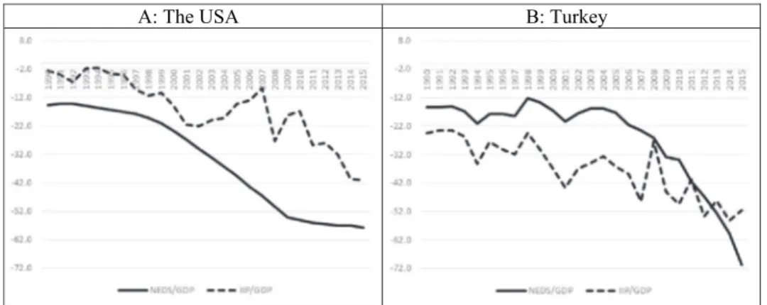
The comparison of the IIP and NEDS (Figure 1) reveals IIP’s weaknesses and the NEDS is proven to be a better indicator. In the USA (Figure 1(a)), for example, both IIP to GDP ratio (from −2.5% to −21.6%) and NEDS to GDP ratio (from −14.8% to −26.7%)

deteriorated together between 1990 and 2001, indicating increased risk. Between 2001 and 2007, however, while the NEDS to GDP ratio continued to deteriorate to −46.4%, the IIP to GDP ratio improved significantly to −8,8%. This was largely caused by the significant devaluation of the Dollar, and the improvement in the IIP to GDP ratio failed to capture the increased risk in the face of lager current account deficit during the period, which eventually led to the 2008 crisis. The significant worsening of the IIP to GDP ratio from −8.8% in 2007 to −41% in 2015 was largely due to the significant evaluation of Dollar and did not indicate correspondingly higher risk as the current account to GDP ratio declined during this period. In the same period, the NEDS to GDP ratio increased moderately from −46.4% to −57.7% and portrayed a more realistic picture.

Subasat (2013) reported similar problems in the context of Turkey. Figure 1(b) shows that although the NEDS to GDP ratio deteriorated significantly between 2002 (−17.5%) and 2015 (−70,8%), the IIP to GDP ratio deteriorated modestly (from −36.9% to −51.6%), which was a major inconsistency given that current account deficit to GDP ratio significantly increased during this period. The difference between these two measures reflects exchange rate changes and market valuation differences. If there were no exchange rate changes and valuation differences, NEDS (net external debt stock) and IIP (current real value of the net external debt stock) would be equal to each other. A faster increase in NEDS implies that the investors are making losses since the amount of money they invest (NEDS) in Turkey is smaller than its current value (IIP). This is only possible if foreign investors kept on investing in Turkey despite their significant loses. While it is not unusual for investors to occasional suffer losses, it would be rather peculiar for them to continue to invest in an economy where they make systematic and long-term losses.

The NEDS figures were significantly more consistent with the radical increase in the current account deficit to GDP ratio, which deteriorated from an average of −0,7% between 1990–2002 to an average of −5.3% between 2003 to 2015. The improvement in IIP from −49.4% in 2010 to −40.6% in 2011 where the current account deficit increased from −6.1% to −9.6% of GDP was a particularly noteworthy inconsistency. These inconsistencies could only be explained by the significant value loses of Dollar against

y e k r u T : B A S U e h T : A

Figure 1. Comparison of IIP and NEDS.

Source: Authors’ own calculations based on data from the World Development Indicators

8-'l 8.0 -ı.o m"f-i,ml~ı,..

; ; 8

a

,_____

,

'

,

\

..

'

,_

the other currencies (including TL) and the significant value gains of TL against the major currencies due to excessive capital inflows.

Moreover, in both countries, the IIP fluctuates radically whereas the NEDS is more stable. The year-to-year variations are so significant as to make IIP an unreliable measure of accumulated risk. In Turkey, for example, the IIP ratio experienced a radical improve-ment from −48,5% in 2007 to −27.4% in 2008 which deteriorated back to −44.9% in 2009 and −49.4% in 2010. Clearly, variations in nominal exchange rates do not help us to get a clear picture of the real risk in an economy.

The above arguments imply that a modified version of NEDS can be used as a more reliable measure of the risk associated with external borrowing.

An alternative risk index

After discussing the weaknesses of the existing risk measures, we can begin to develop our alternative measure, which will be based on an adjusted version of NEDS. Since our index will show the long-term risk level, we change the sign of NEDS by multiplying it by minus one. An increase in NEDS, therefore, will now indicate an increase in risk.

As long as GDP grows faster, a large NEDS will create no major problems since the economy is generating enough income to service its debt. The NEDS to GDP ratio, therefore, is a reasonable baseline measure of long-run risk associated with external borrowing. Several adjustments, however, are required to make the index more accurate since a relatively small NEDS to GDP ratio may be considered excessive in one country, whereas a relatively large NEDS to GDP ratio may be reasonable for another country depending on several factors that will be discussed below.

First, because the nominal GDP is heavily influenced by exchange rate changes, an adjusted GDP (AGDP) measure will be used. It is essential to eliminate the influence of temporary real exchange rate movements since over/under-valuation of exchange rates artificially increases/decreases the nominal GDP and accordingly makes the risk (mea-sured by NEDS to GDP ratio) appear smaller/larger than they actually are. For example, when an economy experiences large capital inflows, real exchange rates tend to be overvalued, causing nominal GDP to be artificially larger and NEDS to GDP ratio to be smaller, leading to real risk being underestimated. When an economy encounters a crisis, however, capital outflows lead to a rapid depreciation of exchange rates, the nominal GDP declines, and NEDS to GDP ratio overshoots, leading to an exaggeration of the actual risk. To resolve this problem, we adjust the nominal GDP by dividing it by a price index (PI) we have developed, so that nominal GDP will not be affected by fluctuations in exchange rates.

AGDP ¼ GDP = PI

We will name the NEDS to AGDP ratio as the Debt Index (DI).

DI ¼ NEDS = AGDP

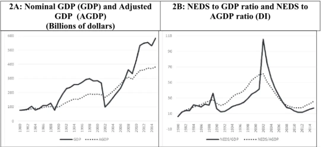
While the technical details of the PI, AGDP and DI (which may not concern the average reader) are explained in the appendix, the following example will demonstrate their usefulness. Argentina experienced excessive capital inflows between 1990 and 2000, leading to over-valuation of the real exchange rate and significantly inflating nominal

GDP figures (Figure 2(a)). AGDP, however, indicates a mild increase. The large gap between these two figures suggests that the nominal GDP was artificially inflated by overvalued exchange rates. Despite Argentina experienced large current account deficits since 1990, NEDS to GDP ratio declined until 1993 (Figure 2(b)) due to the artificial increase in nominal GDP. While NEDS to GDP ratio started increasing since 1993, it remained lower than the NEDS to AGDP ratio (DI) and underestimated the true risk associated with the large current account deficits. During the 2001 and 2002 crisis, nominal GDP declined drastically, not only due to the decline in real production but also due to the collapse of the Argentine Peso. This time NEDS to GDP ratio overshot and increased by 153% between 2001 and 2002 and exaggerated the true risk. The NEDS to AGDP ratio, however, indicates a more stable path and shows the true risk more accurately. It remained higher than the NEDS to GDP ratio (indicating a higher risk) between 1990 and 2000 and indicated no erratic increase during the crisis.

The above example clearly demonstrates the importance of eliminating the artificial changes in nominal GDP due to real exchange rate over-undervaluation.

Second, as discussed earlier, the sustainability of external debt should be assessed in terms of creating favourable conditions for debt service, which requires the productive use of external resources to build economic capacity. While many writers (Reisen, 1998) are mostly concerned with how the current account deficit is financed (i.e., FDI, portfolio investment or external debt), how resources are used is equally (if not more) important.

Long-term economic growth will be driven by higher investment levels and debt service will depend on exports. If external resources are used to stimulate the right type of investments and exports, the debt service will be less problematic. However, if they are used to finance unproductive (speculative) investment, consumption and eco-nomic activities that do not support exports (such as infrastructure and real estate), they will create more risk. We construct a new index to measure such additional risk, which

2A: Nominal GDP (GDP) and Adjusted GDP (AGDP)

(Billions of dollars)

2B: NEDS to GDP ratio and NEDS to AGDP ratio (DI)

Figure 2. The impact of real exchange rate on GDP and NEDS to GDP ratio in Argentina.

Note: Positive NEDS to GDP ratios indicate higher risk.Source: Authors’ own calculations based on data from the World Development Indicators.

600 110 500 400 300 200 100 - GDP ••••••AGDP - NEOS/GD? •••••• NEDS/AGDP

will be termed the Misappropriation Index (MI). The MI is calculated by dividing the annual current account balances (CA) by the annual fixed investment (I) and exports (X).

MI ¼ CA = I þ Xð Þ:

A few adjustments are required to increase the accuracy of this index. First, since exchange rate volatility affects not only nominal GDP, but also nominal investment and exports, the method used to adjust the nominal GDP will be used for nominal investment and exports. Second, residential investment will be excluded from the total investment, as it does not increase productive assets and is often associated with bubbles that lead to an economic crisis.8 Third, rather than gross exports, domestic value added in gross exports will be used. This is necessary because nominal exports exaggerate the real values created in the export sector, due to the increase in the volume of global value chains and the increasing import dependency of exports. The total value of exports may increase, but if the import content of exports increases sufficiently, the value created in the export sector may actually decrease.

The MI generally takes values between 0 and 1 and captures the proportion of external resources used to increase productive investment and promote exports. The larger the investment and exports the smaller the risk associated with external borrowing. The DI and MI are meaningful risk measures separately but the overall risk index (RI) could also be created by combining them. This could be done by multiplying the DI and MI, and adding the results to the DI (see appendix for details).9

RI ¼ DI þ MI x DIð Þ

In the case of Greece (Figure 3(a)), for example, both the DI and the MI increased rapidly between 2004 and 2008. The RI, therefore, increased faster than the DI, indicating a greater risk associated with an unproductive use of external resources. Since 2008, however, the MI has declined rapidly, while the DI continued to increase until 2012 as the current account deficit to GDP ratio remained high. The increase in the DI slowed down as current account deficit to GDP ratio rapidly declined since 2012. The RI also started declining from 2012 and equalized to the DI, since the MI became very close to zero. It is clear from the above figures that the RI captures the real risk better than the DI since external resources in Greece were largely used to finance unproductive economic activities. y e k r u T : B 3 e c e e r G : A 3

Figure 3. Misappropriation Index (MI), NEDS/AGDP Ratio (DI) and Risk Index (RI). Source: Authors’ own calculations based on data from the World Development Indicators

250 200 150 100 50

..

···

·-

..

·

..

···.

.··

..

.

.. ····

·

....

··

··

...

····•

....

·

·

...

The situation in Turkey (Figure 3(b)) is not as grave as Greece, but this is no comfort for Turkey for three reasons. First, Greece is an outlier in terms of risk associated with external borrowing and suffered the most from the 2008 crisis. Second, all risk indicators increased rapidly in the early 2000s. The RI began to decline slightly since 2014 due to the decline in the MI, but the increase in the DI only slowed down since Turkey continued to have a large current account deficit. Turkey, therefore, is still at great risk.

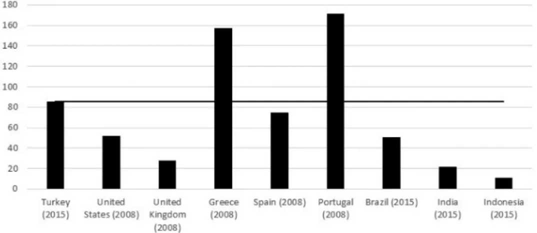
Third, comparing Turkey’s RI with a selection of developed countries that suffered from the 2008 crisis (the USA, the UK, Greece, Spain, Portugal) and the so-called Fragile Five (Turkey, Brazil, India, South Africa, Indonesia) reveals the severity of the risk in Turkey.10 This comparison is significant because Turkey had a higher RI in 2015 than the USA, the UK and Spain in 2008 (when they experienced their crisis) and Fragile Five countries in 2015.

Before concluding this section, it is important to emphasize that, it is neither possible nor necessary to identify a precise benchmarking level for the sustainability of the current account deficit (external debt). It is not possible because setting a benchmark is inevitably subjective.11 It is unnecessary because long-run risk (underlying causes) turn into a crisis due to many short-run factors (triggers) such as political problems and global economic tendencies. In our view, it is a more meaningful exercise to measure the long-term risk without making any judgements about the timing of a crisis.

Estimating the potential welfare loss in Turkey

By using 30 countries with full data, this section investigates the empirical link between the RI and the total adjustment cost of crisis (AC) and uses the regression results to estimate the potential AC for Turkey in case of a crisis. The AC is measured by using the cumulative yearly deviation of household final consumption expenditure (PPP constant 2011 international $) growth in the crisis period from its pre-crisis growth average (see appendix for technical notes).

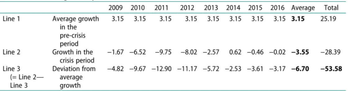
In the case of Greece, for example, the AC is calculated by the following example in

Table 1. The average (normal) consumption growth in the pre-crisis period (1990–2008) was 3.15% (line 1). The average consumption growth in the crisis period (2009–2016) was −3.55% (line 2). This implies that Greece’s consumption during the crisis years annually grew by 6.7% (−3.55–3.15 = −6.7) below its normal growth rate. Since the annual cost is 6.7%, the total AC of crisis for 8 years is −53.58% (= 8 x − 6.7). The same figure could also

Table 1. Calculating the adjustment cost of the crisis in Greece.

2009 2010 2011 2012 2013 2014 2015 2016 Average Total

Line 1 Average growth

in the pre-crisis period

3.15 3.15 3.15 3.15 3.15 3.15 3.15 3.15 3.15 25.19

Line 2 Growth in the crisis period −1.67 −6.52 −9.75 −8.02 −2.57 0.62 −0.46 −0.02 −3.55 −28.39 Line 3 (= Line 2— Line 3 Deviation from average growth −4.82 −9.67 −12.90 −11.17 −5.72 −2.53 −3.61 −3.17 −6.70 −53.58

be calculated by using the cumulative annual deviation of actual growth from average pre-crisis growth (line 3). The formula to calculate the total adjustment cost:

AC ¼ AGC AGPC�xT (1)

−53.58 = (−3.55–3.15) x 8 where

AC: Total adjustment cost of the crisis

AGC: The average growth rate in the crisis period. AGPC: The average growth rate in the pre-crisis period. T: Duration of the crisis (number of years).

Establishing a strong empirical link between the AC and the RI would allow us to estimate Turkey’s expected AC by considering the size of its RI. For this end, we first estimate the following regressions by using the data from 30 countries. Our regressions take the following forms:

1. AC = f (RI) 2. AC = f (RI, HP) 3. HP = f (RI) 4. AC = f (RI, HP*) Where

AC: Total adjustment cost of the crisis RI: Risk index

HP: Percentage change in housing prices between 2008 and 2016.

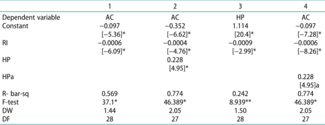
HP*: Percentage change in housing prices between 2008 and 2016 (adjusted for RI). The first regression in Table 2 establishes a strong link between the AC and the RI. The variation in RI accounts for almost 57% of the variation in AC in these countries. To improve the predictive power of the regression, a new index (HP) measuring changes in housing prices in the post-crisis period (2008–2015) will be added to the regression. The RI is expected to illuminate the AC only after a crisis begins and the collapse of housing prices is one of the most obvious signs of the crisis. The RI and HP together account for 77.4% of the AC in these countries (second regression). The coefficients in this regression will be used to estimate Turkey’s AC.12 The cost function is:

Table 2. Regression results.

1 2 3 4 Dependent variable AC AC HP AC Constant −0.097 [−5.36]* −0.352 [−6.62]* 1.114 [20.4]* −0.097 [−7.28]* RI −0.0006 [−6.09]* −0.0004 [−4.76]* −0.0009 [−2.99]* −0.0006 [−8.26]* HP 0.228 [4.95]* HPa 0.228 [4.95]a R- bar-sq 0.569 0.774 0.242 0.774 F-test 37.1* 46.389* 8.939** 46.389* DW 1.44 2.05 1.50 2.05 DF 28 27 28 27

*significant at the one-percent level **significant at the ten-percent level

AC =-0.352 C-0.0004 RI + 0.228 HP

Turkey’s RI was already calculated above (Figure 4) but since Turkey is yet to experience a fully-fledged crisis, the changes in housing prices are not yet known and should be estimated by using the experiences of a number of countries affected by the 2008 crisis. For example, if HP in Turkey declines as much as it did in the UK, the AC in Turkey is expected to be −18.98%.13 If HP declines in Turkey as much as Greece, however, the AC is expected to be −27.86%. From these figures, Turkey’s estimated post- crisis average annual consumption growth rates can be calculated and compared with pre-crisis growth rates. Since the duration of a potential crisis is also unknown, AC will be calculated for 1 year (short but severe crisis), 3 years (longer but milder crisis) and 8 years (very long stagnation) by using the following formula, which is driven from the equation 1.

AGC¼ðAC=TÞþAGPC (2)

If adjustment lasts for 1 year −14.78 = (−18.98/1) +4.19 If adjustment lasts for 3 years −2.13 = (−18.98/3) + 4.19 If adjustment lasts for 8 years 1.82 = (−18.98/8) + 4.19

If HP declines in Turkey as much as the UK, and the crisis lasts only a year, consumption in Turkey is expected to decline by 14.78%. If the crisis lasts 3 years, the yearly consumption growth rate will be −2.13%. And if the crisis lasts 8 years, the yearly consumption growth rate will be 1.82%. Table 3 presents Turkey’s alternative AC calculations and annual growth rates based on the HP experiences of a number of countries. If HP declines in Turkey as much as Greece, the figures are −23.66%, −5.09% and 0.71% respectively. Subasat (2017) suggests that the housing bubble in Turkey is likely to be higher than the UK and the USA but likely to be smaller than Greece. If average HP for the group is used, the more realistic figures are −17.98%, −3.20% and 1.42% respectively. These figures portray a dreadful adjustment for Turkey, which has not been experienced before.

Figure 4. RI in Turkey and selected countries.

Source: Authors’ own calculations based on data from the World Development Indicators

180 160 140 120 100 80 60 40 20 o Turkey (2015)

1

1

1

1

1

-Spain (2008) Portugal Brazil (2015) lndia lndonesia

Conclusion

This paper develops an alternative risk index based on the current account balances. Our index goes beyond whether/when a country is likely to experience a crisis and aims to measure long-term risk and the necessary adjustment cost (welfare loss) in terms of their depth and length. Since the borrowed recourses will be serviced, there will be inevitable welfare loses in terms of declining consumption levels. These losses will be lower or higher depending on the level of total external debt as well as where the borrowed resources are employed. An increase in RI results in an increase in eventual welfare loss.

The accuracy of the RI was tested by using 30 countries with full data. Our risk index successfully explained 57% of the variation in the welfare loss in these countries. Adding changes in house price index into the regression significantly improves the results and explains 77.4% of the variation in welfare loss. These are very significant results con-firming the accuracy of our study.

The regression results were also used to estimate the potential welfare loss for Turkey once a crisis begins. Our results suggested that consumption in Turkey is likely to decline between 14.78% and 23.86%. These figures portray a dreadful welfare loss for Turkey, which has not been experienced before.

It is unlikely but possible for Turkey to temporarily postpone a fully-fledged crisis by attracting further international capital inflows. Turkish Lira experienced similar (but less severe) pressures in 2015, 2016 and in May 2018 but interest rates were increased sufficiently to curb capital flights and stabilize exchange rates. Improvements in the global economic environment, such as a favourable change in FED’s interest rate policy and a decline in oil prices, could also help. Normalizing the relations with the EU and the USA would ease the tensions.

Turkey also received very large capital inflows from anonymous sources since 2002, which have enhanced the resilience of the economy against various shocks. These flows intensify considerably during the election years and when the economy experiences problems. The cumulative unaccounted net capital inflows into Turkey since 2003 reached 57.8 USD billion. In the first ten mounts of 2018 alone Turkey received 18.4 USD billion of anonymous capital, which is by far the largest amount in one year. Subasat (2017) argued that the official figures significantly underesti-mate the real unaccounted capital inflows and estiunderesti-mates the actual figures to be four to twenty times larger.

Table 3. Turkey’s potential AC under alternative scenarios.

AC 1 year 3 years 8 years

The UK −18.98 −14.78 −2.13 1.82 France −19.55 −15.36 −2.32 1.75 The USA −19.80 −15.61 −2.41 1.72 Iceland −20.22 −16.03 −2.55 1.67 Portugal −20.97 −16.78 −2.80 1.57 Average −22.18 −17.98 −3.20 1.42 Italy −23.83 −19.64 −3.75 1.21 Spain −26.19 −22.00 −4.54 0.92 Greece −27.86 −23.66 −5.09 0.71

None of the above, however, could resolve Turkey’s problems. While postponing the crisis, they would only aggravate the situation and increase future welfare loss. Turkey is like a vehicle going downhill without brakes. The sooner the necessary adjustment is, the lesser the damage will be.

Notes

1. An example will clarify the issue. In 2012 Turkey received $69 billion net capital inflows ($62 billion capital account surplus and $9 billion net errors and omissions) which financed $45 billion of current account deficit and the remaining $24 billion was stored as reserves. Since reserves could be used to service the debt they created no risk and only $45 billion that was used to finance the current account deficit created real liabilities. Although the capital account surplus was $62 billion and the total capital inflows were $69 billion, the risk increased only by $45 billion.

2. In the above example (footnote 1), for example, it would be inaccurate to argue that $24 billion reserves in Turkey would reduce the risk associated with the $45 billion current account deficit.

3. See Subasat (2016) for a wide range of alternative crisis theories.

4. Although the IIP covers all liabilities created by external debt, liabilities section in the IIP is broader than the external debt. See IMF (2014) for further details.

5. It is indeed true that the current investment value could be very different from the initial investment value. For example, a foreign investor could bring $1 million into a country but after a year, the total value of the investment could increase (to $2 million) or decrease (to $0.5 million).

6. The Balassa Samuelson Effect, for example, suggests that exchange rates tend to appreciate due to faster productivity increases in exportables than the overall economy.

7. For example, assume that net errors and omissions are zero, exchange rates and market valuations remain unchanged and that a country has a capital account surplus of $100 billion in a particular year. Assume further that $70 billion is used to finance the current account deficit and remaining $30 billion is stored as reserves. Although the country borrowed $100 billion, the increase in IIP is equal to $70 billion, as $30 billion of this debt can be paid by resources added to reserves. Therefore, the change in IIP is equal to $70 billion, which is equal to the current account deficit of that year.

8. See Roberts (2011) for the justification of this decision.

9. Note that creating a composite index is inevitably subjective. See for example the contro-versies over how the famous Human Development Index is calculated (Klugman, Rodríguez, and Choi, 2011). Our main indicator here is the DI and we use MI to modify it. As can be seen in Figure 3, when MI increases, RI increases more than the DI, indicating a higher risk and when MI is equal to zero, DI and RI are equal to each other.

10. South Africa is excluded due to insufficient data.

11. Reisen (1998), for example, identifies a rather arbitrary sustainable cumulative current account deficit level of 50%.

12. To see a more realistic picture regarding the relative impacts of RI and HP, the regression should be refined by considering the collinearity between the independent variables. Regression 3 shows that RI and HP are collinear. In order to resolve this issue, the residuals from this regression are saved as adjusted HP index (HP*) and used in regression 4 to get a better picture. As is clear from the R-bar-squares and F-tests, regression 2 and 4 will yield the same results except for the coefficients of the variables. Both results could be used to estimate Turkey’s AC but regression 2 will be preferred since HP* is not directly observable.

13. Subasat (2017) compares housing price changes in Istanbul with New York and London and argues that average housing prices have increased faster and longer time period in Istanbul

than those two cities. It is therefore reasonable to assume that the imminent housing price collapse will likely to be more severe.

Disclosure statement

No potential conflict of interest was reported by the authors.

Notes on contributors

Soner Uysal is a Ph.D. student and a research assistant at Muğla Sıtkı Koçman University. He has published books and articles in the fields of international trade, international economic policies, national asset funds, and foreign direct investments.

Turan Subasat is a professor at Muğla Sıtkı Koçman University. He received his B.Sc. from the University of Istanbul, his M.Sc. (Birkbeck College) and Ph.D. (SOAS) from the University of London, UK. He previously taught development studies at the University of London (SOAS), economics at the University of Bath, UK and economics at the Izmir University of Economics, Turkey. His research focuses on development, international and political economics. He has published in political economy journals including the Review of Radical Political Economics and Journal of Balkan and Eastern Studies. He edited a book titled The Great Financial Meltdown: Systemic, Conjunctural or Policy-Created? Published by Edward Elgar in 2016.

References

Agosin, R.M. (1994), Saving and Investment in Latin America, UNCTAD Discussion Paper No. 90, Geneva.

Corsetti, G., Pesenti, P. and Roubini, N. (2001), Fundamental Determinants of the Asian Crisis: The Role of Financial Fragility and External Imbalances’, in T. Ito and A. Krueger (eds),

Regional and Global Capital Flows: Macroeconomic Causes and Consequences, National

Bureau of Economic Research.

Glick, R. and K. Rogoff (1995), Global versus country-specific productivity shocks and the current account, Journal of Monetary Economics, 35.

Grabel, I. (1996), Marketing the Third World: The Contradictions of Portfolio Investment in the Global Economy, World Development, Vol. 24 (11).

IMF (2014), External Debt Statistics: Guide for Compilers and Users, Inter-Agency Task Force on Finance Statistics, IMF, Washington, D.C.

Irandoust, M. and J. Ericsson (2004), Are imports and exports cointegrated? An international comparison. Metroeconomica, 55

Klugman J., F. Rodríguez and H-J. Choi (2011), The HDI 2010: New Controversies, Old Critiques, Journal of Economic Inequality, 9 (2)

Milesi-Ferretti, M. G. and A. Razin (1996) Sustainability of persistent current account deficits,

National Bureau of Economic Research Working Paper, (5467).

Nakonieczna-Kisiel, H. (2011), ‘International investment position versus external debt’, Folia Oeconomica Stetinensia, Vol 10, Issue 1.

Obstfeld, M. and K. Rogoff (1995), The intertemporal approach to the current account, in G. Grossman and K. Rogoff (eds), Handbook of International Economics, vol. IIl. Elsevier Science.

Ogus, A. and N. Sohrabji (2008), On the optimality and sustainability of Turkey’s current account, Empirical Economics, 35.

Razin, A. (1995), The Dynamic-Optimizing Approach to the Current Account: Theory and Evidence, in P. B. Kenen (ed.), Understanding Interdependence: The Macroeconomics of the Open Economy, (Princeton University Press).

Reisen, H. (1998), Sustainable and Excessive Current Account Deficits, Empirica, Vol 25 (2). Reisen, H. (2000), Pensions, Savings and Capital Flows: From Ageing to Emerging Markets,

(Cheltenham: Edward Elgar and OECD).

Roberts, M. (2011), Measuring the rate of profit, profit cycles and the next recession, AHE Conference, July 2011

Sissoko, Y. and J. J. Jozefowicz (2016), An Investigation of Current Account Sustainability in Five Asean Countries, 4(1).

Subasat, T. (2013), AKP’nin Ekonomik Başari Miti 3 - Cari Açik ve Dış Borç, İktisat ve Toplum, No. 36.

Subasat, T. (2016), The Great Meltdown of 2008: Systemic, Conjunctural or Policy-created?, (London: Edward Elgar).

Subasat, T. (2017), Turkey at a Crossroads: The Political Economy of Turkey’s Transformation. Markets, Globalization Development Review, Vol. 2: No. 2.

Subasat, T. (2019), The Political Economy of Turkey’s economic miracles and crisis, in E. Parlar (ed.), Turkey’s Political Economy in the 21st Century, (London: Palgrave Macmillan)

Turan, Z. and D. Barak (2016), ‘Türkiye’de Cari İşlemler Açığının Sürdürülebilirliği’, İşletme ve İktisat Çalışmaları Dergisi, 4 (2): 70–80

Utkulu, U. (1998), “Are the Turkish External Deficits Sustainable? Evidence from the Cointegrating Relationship Between Exports and Imports”, DEU. IIBF. Dergisi, 13 (1),119–32.

Uysal, S. (2016), Cari Açıkların Sürdürülebilirliğine İlişkin Yeni Bir Yaklaşım: Cari Açık Risk Endeksi Uygulaması, (Unpublished master thesis). University of Mugla Sitki Kocman, Mugla, Turkey.

Appendix

For all variables, t and j denote year and country respectively. Adjusted GDP (Y�

tj) is calculated by dividing nominal GDP Ytj

�

by the price index we have developed (PItj):

Y�

tj¼

Ytj

PItj

The price index ðPItjÞis calculated by dividing a country’s price deflator (Ptj) by the US price

deflator (PtUSA) and indexing it to 1990. The price deflator is calculated by dividing nominal GDP

by real GDP.

PI1990j¼ Ptj

P1990j=

PtUSA

P1990USA

Debt Index ðDItjÞis calculated by a ratio of NEDS to Ytj�:

DIij¼

NEDS

Y�

ij

The formula for NEDS:

NEDS ¼

Xt t¼1990

CAtj

MItj¼

CAtj

IHtjþXVtj

Where CAtj is current account deficit, IHtj is investment (I) net of residential investment (H) and

XVtj is domestic value added in gross exports. XVtj and IHtj are adjusted by the price index (PItj).

The overall risk index (RI) is created by combining DI and MI with the following formula:

RItj¼ DItjþ DItjMItj

�

The cost of crisis or adjustment cost (AC) indicates the loss of household consumption during the crisis. Household consumption expenditures are taken into account to calculate this cost. AC is the sum of the difference between growth in post-crisis consumption PostCGRtj

�

and the average growth in pre-crisis consumption ðPreACGRtjÞ.

AC ¼X Post CGRtj Pre ACGRtj