Impact of liquidity on stock returns listed in Borsa Istanbul

(1)

IMPACT OF LIQUIDITY ON STOCK RETURNS LISTED IN

BORSA ISTANBUL

A Master’s Thesis

by

NERMİN EMRAH

Department of Management İhsan Doğramacı Bilkent University

Ankara August 2015

(2)

IMPACT OF LIQUIDITY ON STOCK RETURNS LISTED IN

BORSA ISTANBUL

Graduate School of Economics and Social Sciences of

İhsan Doğramacı Bilkent University

by

Nermin EMRAH

In Partial Fulfilment of the Requirements for the Degree of MASTER OF SCIENCE

in

THE DEPARTMENT OF MANAGEMENT İHSAN DOĞRAMACI BİLKENT UNIVERSITY

ANKARA August 2015

(3)

I certify that I have read this thesis and have found that it is fully adequate, in scope and in quality, as a thesis for the degree of Master of Science in Management.

--- ---

Assoc. Prof. Aslıhan Altay-Salih Assist. Prof. A. Başak Tanyeri

Supervisor Co-Supervisor

--- Assoc. Prof. Levent Akdeniz Examining Committee Member

--- Assist. Prof. Seza Danışoğlu Examining Committee Member

Approval of the Graduate School of Economics and Social Sciences

--- Prof. Erdal Erel

(4)

iii

ABSTARCT

IMPACT OF LIQUIDITY ON STOCK RETURNS LISTED IN

BORSA ISTANBUL

Emrah, Nermin

M.S., Department of Management Supervisor: Assoc. Prof. Aslıhan Altay-Salih Co-Supervisor: Assist. Prof. A. Başak Tanyeri

August 2015

This study investigates the impact of liquidity on returns of stocks traded at Borsa İstanbul for the 2002-2014 period. Turnover rate, which is defined as average volume of a firm divided by the number of shares outstanding of that firm, is used as a liquidity measure. Liquidity effect is examined following panel data analysis and robust estimators controlling the effect of well-known firm-specific characteristics. The results show that turnover rate has a significant and negative effect on stock returns. This result indicates that investors request compensation for holding illiquid assets. In other words, they request compensation for the assets with low turnover. The impact of turnover rate on stock returns is significant for the whole year; therefore, results are not driven by the January effect.

(5)

iv

ÖZET

LİKİDİTENİN İSTANBUL BORSASINDA İŞLEM GÖREN HİSSE

SENETLERİNİN GETİRİLERİ ÜZERİNDEKİ ETKİSİ

Emrah, Nermin

Yüksek Lisans, İşletme Bölümü Tez Yöneticisi: Doç. Dr. Aslıhan Altay-Salih

Ortak Tez Yöneticisi: Yrd. Doç. Dr. Prof. A. Başak Tanyeri

Ağustos 2015

Bu çalışma, likiditenin 2002 ve 2014 yılları arasında Borsa İstanbul’da işlem gören hisse senetlerinin getirileri üzerindeki etkisini araştırmaktadır. Likidite ölçütü olarak, şirketin ortalama hacminin piyasada dolaşan hisse senedi sayısına bölümü ile elde edilen devir hızı kullanılmaktadır. Devir hızının etkisi bilinen şirkete has karakteristikler kontrol edilerek panel veri analizi ve sağlam tahmin ediciler ile incelenmiştir. Sonuç olarak devir hızının hisse senedi getirisi üzerinde negatif ve anlamlı bir etkisi olduğu görülmüştür. Bu sonuçtan, yatırımcıların likit olmayan varlıklar için telafi talep ettikleri anlaşılmaktadır. Diğer bir ifadeyle, yatırımcılar devir hızı düşük varlıklar için telafi talep etmektedirler. Çalışmada, devir hızının hisse senedi getirisi üzerindeki etkisinin yılın tamamı için anlamlı olduğu ve dolayısıyla sonucun Ocak etkisinden kaynaklanmadığı anlaşılmaktadır.

(6)

v

ACKNOWLEDGEMENTS

I am thankful to my supervisor Assoc. Dr. Aslıhan Altay-Salih for her guidance throughout this work. Without her stimulating suggestions and patience, it would be impossible to complete this thesis.

I would like to thank Assist. Prof. A. Başak Tanyeri, my co-supervisor, for her support to this study.

I am also grateful to Assoc. Prof. Levent Akdeniz and Assist. Prof. Seza Danışoğlu for examining my study and participating at the examining committee during summer holiday.

I would like to thank my family for the support they provided whenever I needed. Without their unconditional support, trust and love, it would have been impossible to achieve any accomplishment throughout my life.

Finally, I would like to thank TÜBİTAK for the financial support they provided for my graduate study.

(7)

vi

LIST OF TABLES

Table 1 - Number of stocks ... 46

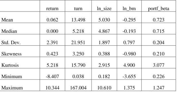
Table 2 - Descriptive statistics for variables ... 49

Table 3 - Pairwise correlations ... 49

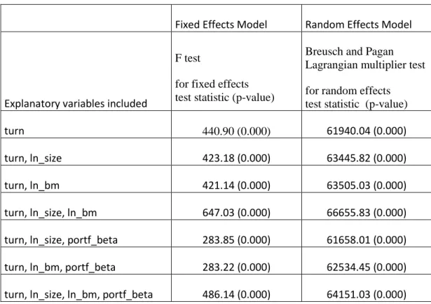
Table 4 - F test and LM test ... 51

Table 5 - Testing heteroskedasticity ... 52

Table 6 - Testing serial correlation ... 53

Table 7 – Regression coefficients ... 55

Table 8 – Regression coefficients of model with momentum ... 57

Table 9 - Testing January effect ... 59

(10)

ix

LIST OF FIGURES

Figure 1 - Graph of excess gross returns and relative spread (A&M;1986) ... 12 Figure 2 - Graph of relative asset value and relative spread (A&M;1986) ... 13 Figure 3 - Panel data modeling process ... 45

(11)

1

CHAPTER I

INTRODUCTION

Liquidity, which is basically defined as the ease of buying and selling an asset at the current market price immediately and at low cost, is generally considered as one of the important determinants of asset prices. The link between stock returns and liquidity of stocks has been recognized since Amihud and Mendelson (1986).

Amihud and Mendelson (henceforth, A&M) investigate function of liquidity in capital markets by concentrating on the impact of illiquidity on stock price. It is the very first study presenting the existence of a relation between asset prices and liquidity theoretically. They firstly theoretically model the role of the bid-ask spread on asset returns. Their model indicates that assets which have high bid-ask spread yield higher expected returns compared to the assets with low bid-ask spread. They also introduce clientele effect which proposes that investors having longer holding periods are inclined to hold higher-spread assets. The first testable hypothesis of the theory is assets with higher spread yield higher returns, leading investors whose expected holding periods are longer to invest in holding higher-spread assets. The second testable hypothesis is in equilibrium, observed market return is found to be an increasing, piecewise-linear and concave function of the bid-ask spread with respect to holding periods of investors.

(12)

1

The study of A&M (1986) led many researchers to study the liquidity premium. In the post 1986 period, relation between asset returns and stock illiquidity has become the subject of numerous empirical studies. However, results obtained from these studies are mixed; i.e. while some of the papers suggest that illiquidity has positive effect on expected asset returns (e.g. Eleswarapu (1997), Datar, Naik and Radcliffe (1998), Hu (1997), Brennan, Chordia and Subrahmanyam (1998), Chordia, Subrahmanyam and Anshuman (2001), Amihud and Mendelson (1991), Marshall and Young (2003), Chan and Faff (2003)), others do not find evidence on existence of positive illiquidity premium (e.g. Rouwenhorst (1999), Chalmers and Kadlec (1998), Lischewski and Voronkova (2012), Donadelli and Prosperi (2012)); and some find mixed results such as liquidity effect is only significant at January due to seasonal effect (e.g. Eleswarapu and Reinganum (1993), Brennan and Subrahmanyam (1996)).

Mixed outcomes obtained in the previous studies may be linked to usage of low frequency and often limited data. Amihud, Mendelson and Pedersen (2006) pointed out that empirical studies are restricted due to non-availability of informative data. They claim that illiquidity resulting from market microstructure can only be examined with high frequency data which is available recently and thus data for very short period can be used. Therefore, researchers need data with lower frequency such as daily trading volume or return data provided that they are faced with problem of having limited high frequency data.

Obtaining different outcomes from empirical studies could also be related to usage of different liquidity measures. Liquidity is a complex concept with various determinants such as cost of immediate execution, information asymmetry, brokerage commissions and transaction taxes. As no single measure of liquidity which captures all of these aspects is known, developing a single measure of illiquidity is difficult.

(13)

2

Therefore, empirical studies employ different measures to study return-liquidity relation. As previous literature does not enable us to derive concrete results about the existence of liquidity effect, this area is interesting for further investigation.

Moreover, most of the previous studies focus on US markets, the most liquid market in the world. However, emerging countries are more likely to face with problems caused by illiquidity. Lesmond (2005), examines the effect of political institutions and legal origin on levels of liquidity, and suggests that liquidity cost in countries having weaker legal and political institutions is significantly higher.

This thesis aims to investigate the relationship between stock returns and liquidity by examining returns of stocks traded at Borsa İstanbul for the 2002-2014 period. For this purpose, turnover rate is used as liquidity measure. Turnover rate is calculated as the number of shares traded as a fraction of the number of shares outstanding.1 Choice of turnover rate as a liquidity measure is due to the inversely proportionality of turnover rate to holding period of investors (Datar, Naik and Radcliffe (1998)).2 When holding period of an asset is low, it is expected that its turnover rate of that asset is high. This relation between holding periods and turnover rate indicates turnover rate as an appropriate measure of liquidity. As theory of A&M proposes the existence of positive relationship between spread (stock illiquidity) and stock returns, the relationship between liquidity of stocks and returns should be negative. Therefore, the testable hypothesis of this study is that there is a statistically significant and negative relation between turnover rate and stock returns.

1_{Some of the studies using turnover rate as liquidity measure are Datar, Naik, and Radcliffe (1998),} Rouwenhorst (1999), Chordia, Subrahmanyam and Ansuman (2001) and Nguyen, Mishra, Prakash and Gosh (2007).

2_{Holding period is defined as number of outstanding shares divided by average volume by Atkins and} Dyl (1997)

(14)

3

In this study, turnover rate is an informative measure for a stocks’ liquidity listed at Borsa İstanbul considering relatively short holding periods in volatile emerging stock markets. Turkey, being an emerging economy, will provide more appropriate setting to investigate the effect of liquidity, if such effect exists. Therefore, I aim to contribute to the discussion about the presence of liquidity impact on stock returns by gathering evidence beyond the already documented by the empirical studies conducted in developed markets.

Another strength of this study is the usage of daily data in the analysis rather than monthly data differing from most of the previous studies. By examining daily stock returns, I attempt to reveal more informative results on the existence of liquidity effect on stock returns compared of Turkish stocks as this market is characterized by highly variable daily liquidity.

Results of the analysis document that there is a negative and statistically significant effect of liquidity on stock returns for stocks traded at Borsa İstanbul during the 2002-2014 period. Investors require more returns for a compensation of holding an illiquid security. Results support the existence of liquidity premium for stocks traded at an emerging economy. This finding is consistent with the A&M’s (1986) theory. Also, as the effect of liquidity persists for the whole period, it is concluded that the findings are not driven by the seasonal effect.

Significant and negative effect of turnover rate on stock returns remains stable after controlling for the well-known firm-specific attributes such as size of firm, book-to-market ratio and beta. As expected, size affects significantly negatively stock returns, while book-to-market ratio and beta affect returns significantly and positively. Organization of the remainder of the thesis is as follows: Chapter II provides brief information about liquidity; Chapter III summarizes the previous studies; Chapter

(15)

4

IV explains the methodology and dataset; Chapter V presents the analysis and results; and Chapter VI concludes.

(16)

5

CHAPTER II

GENERAL OVERVIEW OF LIQUIDITY

In the simplest term, liquidity is defined as the ease of transacting a security. This term is used to explain how quickly and how easy a stock can be turned into cash. That is, an asset is said to be illiquid when it cannot be immediately sold without having potential for losing significant percentage of its value.

Determination of level of liquidity is a difficult task as there are several aspects that should be considered. For example, as the assets will be issued by different issuer, in equities and corporate bond markets, segmentation of the market is observed. Also, even if an asset will be issued by the same issuer, it may still have different characteristics affecting its liquidity such as different maturities in the market for governmental securities, different voting rights for preference shares, etc. Therefore, liquidity is an important concept in explaining various cases in financial markets. It helps to explain cross-section of assets having various level of liquidity, controlling for other pricing characteristics. It also helps us to understand reasoning behind low prices of securities that are hard to trade, differences in valuation and returns of equities and liquid risk-free treasuries, etc. (Amihud, Mendelson and Pedersen (2006)).

(17)

6

2.1. Determinants of Illiquidity

As it is a complex concept, one should consider various aspects when explaining the reasons of illiquidity of an asset.

First of all, in order to determine an assets’ liquidity, one should measure the cost of immediate execution. As A&M (1986) stated, transaction of assets confronts investors with a tradeoff between transacting immediately at the current bid/ask price or search for favorable price and bear the delay and search costs.

In financial market, liquidity is ensured by brokers and dealers. Role of the dealer is to trade with customers and other dealers. Sellers sell their assets to a dealer or buying assets from a dealer. The price that an asset can be bought is ask price and the price that an asset can be sold is the bid price of the asset. These prices are first quoted by the dealers, then public traders state the prices that they are willing the buy/sell and the quantity of the orders. The transactions are done at the best prices offered. Brokers are responsible in trading of both dealer to dealer and dealer to retail customers. They facilitate the execution by their system in which all bid and ask prices can be seen. Trading via broker ease communication and reduces the searching costs. Of course, in order to have these entire facilities one should bear the additional brokerage commissions.

Another exogenous transaction cost arises from transaction taxes; which is defined as the tax on a sale of a property or financial instrument. As the name suggests, these taxes should be paid when a transaction takes place increasing cost of transaction and decreasing the liquidity of an asset.

The other reason of illiquidity is the increased cost of transaction due to information asymmetry. Asymmetric information is a problem in financial markets. It is a situation in which one party, the buyer or the seller, has superior information than

(18)

7

the other. It is almost inevitable to avoid from losing in a transaction where counterpart has private information about fundamentals of the security transacted such as knowledge of the seller that the company is about to be bankrupted. Another example is that if the buyer knows information about the order flow, he/she can forecast the mobility of the prices for the following period. Therefore, information asymmetry can directly affect the liquidity of an asset.

These costs have to be beard when the investor decides to execute his/her order immediately. As an alternative, he/she can wait for more profitable price. However, this option is also related additional costs which cover the searching for better prices, contacting with traders and delaying the execution. Search and bargaining problems were examined by Duffie, Garleanu and Pedersen (2003), Weill (2002), and Vayanos and Wang (2002).

2.2. Liquidity Premium

Liquidity premium is defined as the excess return expected to be earned on an asset at a given point of time due to its relative market illiquidity. Traders request to be compensated for holding less liquid assets since transaction costs for transacting those assets will be higher compared to the assets with higher liquidity. In other words, in equilibrium, the market where the transaction takes place should provide more liquidity premium to the owners of less liquid assets relative to the owners of more liquid assets.

Existence of liquidity premium is directly associated with the liquidity risk in asset pricing. Throughout the literature, many researchers investigates the capital asset pricing models with presence of liquidity risk (some of these studies are: Lippman and

(19)

8

McCall (1986), Holmstrom and Tirole (2001), O’Hara (2003), Acharya and Pedersen (2005), Liu (2006)).

Isaenko and Zhong (2013) study the liquidity premium in the presence of stock market crises. For this purpose, they analyze the optimal behavior of an investor who invests in a risk-free bond market and the stock market for a long-term. They study a stock market which is liquid in most of the time but not when liquidity crashes occur. Considering transaction costs in order to capture illiquidity, they find that liquidity premium resulting from stock market crises is significant.

(20)

9

CHAPTER III

LITERATURE REVIEW

3.1. Theoretical Model of Amihud & Mendelson (1986)

Although it is known to be an important factor in investment decisions, first theoretical study focusing on this issue has not been published before 1980s.The first and probably the most important paper on this subject is study of A&M (1986).

A&M propose a theoretical model and then validate the hypothesis of the model by empirical analysis. They argue that cost of immediate execution should be considered in order to measure illiquidity of assets. The main consideration of this thesis is studying the impact of illiquidity, measured by bid-ask spread, on asset pricing.

Firstly, they form a model that predicts that high returns are associated with assets having high bid-ask spread. Their model also suggests existence of clientele effect, investors who have longer holding periods buy assets higher bid-ask spread assets. In the formation of the model, they consider the investor types differing by the expected holding periods. They assume that the demand for liquidity is exogenously determined.

(21)

10

Their first proposition (clientele effect) states that in equilibrium, long-term investors hold the assets with higher spreads, i.e. with lower liquidity. The second proposition is related to spread-return relationship, by which they claim increasing and concave relation presents between returns and spread.

A&M define M investor types with indices i=1,2,…,M and N+1 assets with j=0,1,2,…,N. Each asset j is associated with relative spread, Sj.and cash flow $dj per unit time (dj>0).

Assets are assumed to be perfectly divisible. It is also assumed that one unit of each asset is available. Asset 0 is defined as the asset having zero spread (S0=0) with unlimited supply.

As the transaction is done via competitive market makers, each asset’s ask price is defined as Vj, and bid price is defined as as Vj(1-Sj) in order to compensate market makers’ risk resulted from the difference in arrival timing of buyers and sellers to the market. In this context, ask price vector is defined as (V0, V1,…, VN) and bid price vector is defined as (V0, V1(1-S1),…, VN(1-SN)).

Each type-i investor having wealth Wt holds the assets for a random time period, Tt, which is distributed exponentially and have mean E[Tt]=1/µt. Investors are numbered by expected holding periods, 𝜇₁−1 _{≤ 𝜇}

2−1≤ ⋯ 𝜇𝑀−1, and assets are numbered by relative spreads, 0 = 𝑆₀ ≤ 𝑆₁ ≤ ⋯ ≤ 𝑆_𝑁 < 1. An investor sells the asset at the bid prices to the market makers in order to liquidate portfolio he/she holds and leaves the market. It is assumed that arrival of each type of investor is a Poisson process with rate λi, and inter-arrival times and holding periods of investors are independent.

An investor aims to maximize the amount of expected discounted net cash flows received. Expected present value of holding a portfolio is found by summation

(22)

11

of the expected discounted value of the cash stream obtained through the holding period and the expected discounted liquidation revenue:

𝐸_𝑇₁{∫ 𝑒−𝑝𝑦_{[∑ 𝑥} 𝑖𝑑𝑗]𝑑𝑦} + 𝐸𝑇1{𝑒−𝑝𝑇∑ 𝑥𝑖𝑗𝑉𝑗(1 − 𝑁 𝑗=0 𝑁 𝑗=0 𝑇1 0 𝑆_𝑗)} = (𝜇1+ 𝜌)−1∑𝑁𝑗=0𝑥𝑖𝑗[𝑑𝑗+ 𝜇𝑖𝑉𝑗(1 − 𝑆𝑗)] (3.1)

Maximization of this sum (subject to wealth constraint, ∑𝑁𝑗=0𝑥𝑖𝑗𝑉𝑗 ≤ 𝑊𝑖) and calculating expected spread-adjusted returns of asset j to the investor type-i by subtracting expected liquidation cost per unit time (𝑟_𝑖𝑗 =𝑑𝑗

𝑉𝑗− 𝜇𝑗𝑆𝑗) of asset j from the gross market return on that asset, relation between asset returns, relative spread and investor’s holding periods is defined as:3

𝑉_𝑗∗ ₌𝑑𝑗

𝑟_𝑖∗− 𝜇𝑖𝑉𝑗 ∗_𝑆

𝑗/𝑟𝑖∗ (3.2)

Propositions of the paper implied by the above equilibrium relation is followed:

Proposition 1 (clientele effect). Assets with higher spreads are allocated in equilibrium to portfolios with (the same or) longer expected holding periods.

Proposition 2 (spread-return relationship). In equilibrium, the observed market (gross) return is an increasing and concave piecewise-linear function of the (relative) spread.

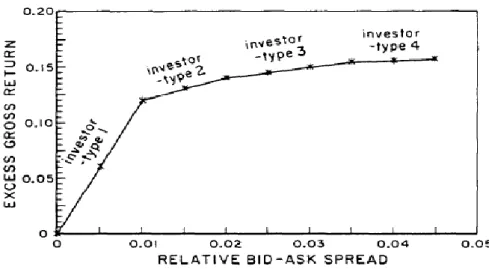
Figure 1 given below is taken from their paper which is an illustration of the main testable implication of the model:

(23)

12

Figure 1 - Graph of excess gross returns and relative spread (A&M;1986)

Figure shows the link between excess gross return and relative bid-ask spread for types of investors as modeled by A&M(1986).

This figure shows piece-wise, positive and concave association between observed market return in excess of the return on zero-spread of assets. This relation results from the compensation requested by investors for holding illiquid assets combined with clientele effect. As transaction costs faced by investors are amortized over their holding period, smaller compensation is required for investors whose holding periods are longer. According to the model, in equilibrium, assets with higher bid-ask spread will be held by investors with longer holding periods; therefore, the added return required against a given unit of increase in transaction cost gets smaller. In this figure, as type-4 investor has longer expected holding period, added return required by him/her is smaller compared to the others.

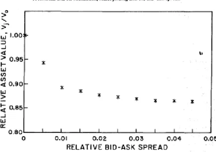
The Figure 2 presented in their study to demonstrate the effect of relative spread on values of assets is given below:

(24)

13

Figure 2 - Graph of relative asset value and relative spread (A&M;1986)

Figure shows the decreasing relation between relative asset prices and relative bid-ask spread as modeled by A&M(1986).

As this figure suggests equilibrium asset values are decreasing the spread in line and this relation is convex.

A&M then test their hypothesis by using the stock returns gathered from NYSE for the 1960-1979 period. Cross-sectional relation between bid-ask spread, stock return and relative risk over time is examined using relative bid-ask spread (dividing dollar spread to the average of the bid and ask prices at the end of the year) as a liquidity measure. Following the Fama-MacBeth (1973) methodology, portfolios are formed by classifying stocks considering their relative risk and spread. Data is divided into 20 overlapping periods each of which consists of 11 years. Beta estimation period is five year, portfolio formation period is five year and test period is one year. Cross-section and time-series is pooled to obtain estimates in order to test the main hypothesis.

(25)

14

Results of the main analysis provide evidence on the validity of their model. In particular, they suggests positive and statistically significant effect of bid-ask spread on risk-adjusted returns present. The slope coefficients of the spreads are found to be positive and gets smaller as moving to group of assets which have higher spread, so the concavity of the return-spread relation actually presents. This is an evidence on the long-term portfolios are less sensitive to bid-ask spreads.

3.2. Study of Datar, Naik and Radcliffe (1998)

Datar, Naik and Radcliffe (1998) proposes a different way to test hypothesis of A&M (1986) by defining turnover rate as a liquidity measure rather than bid-ask spread and show that findings are still consistent with the theory of A&M (1986). Motivation for using turnover rate will be explained in this subsection in detail.

Their dataset includes non-financial firms traded at the NYSE between July 1962 and December 1991. They have 880 stocks for each month on average. Monthly stock returns are obtained from Centre for Research in Security Prices (CRSP).

Turnover rate is computed by dividing the number of shares traded for a stock in a month to the number of shares outstanding in that stock and expressing this value as percentage. Their results provide supporting evidence on the propositions of A&M’s model.

Datar, Naik and Radcliffe (1998) study whether stock liquidity positively affects stock returns as proposed by A&M’s (1986). As in the model of A&M, assets are held by type-i investors for a random time and these assets are sold at the bid price to the market makers and investors leave the market at the end of the time horizon.

The main objective of the study of Datar, Naik and Radcliffe (1998) is to test Proposition 1 and 2 of A&M (1986) jointly. They describe that the turnover rate is

(26)

15

proportional to the inverse of holding periods, variable µ in A&M (1986) model; therefore, since asset return increases expected holding periods increase (according to the A&M model), it also has to be a decreasing function of the turnover rate.

Generalized least squares (GLS) methodology is used to see if differences in turnover rates have explanatory power in explaining observed cross-sectional variation in stock returns. GLS is used as it gives more weight on the slope coefficients; therefore coefficients are estimated precisely even when Gauss Markov assumptions do not hold as explained in detail in the paper.

Model of the Datar, Naik and Radcliffe (1998) is given below:

𝑅𝑖𝑡 = 𝛾𝑜𝑡+ ∑𝐾𝑘=1𝛾𝑘𝑡𝑥𝑖𝑡+ 𝜀𝑖𝑡 (3.3)

where 𝑅𝑖𝑡 is the observed return for stock i on month t, and 𝑥𝑖𝑡 are explanatory variables; and i=1,2,…,Nt where Nt denotes the number of securities in month t.

Response variable is the observed daily return of a stock i on month t; independent variable is turnover rate of a stock i on month t; and control variables are size, book-to-market ratio and beta.

Turnover rate is estimated by calculating average monthly trading volume for a stock (taking average of number of shares traded during the previous three months; t-3, t-2, t-1), dividing this by the number of outstanding shares of that firm and expressing this ratio by percentage.

They follow Litzenberger and Ramaswamy’ (1979) methodology, an improved version of the Fama-MacBeth (1973). Litzenberger and Ramaswamy (1979-pp. 174-175) propose that when estimators 𝛾̂𝑘𝑡 for 𝛾𝑘𝑡, k=0,1,2,3 or 4 are not serially correlated, the pooled GLS estimator 𝛾̂_𝑘 can be obtained by calculating the weighted mean of the estimates.

𝛾̂_𝑘 = ∑𝑇 𝑍_𝑘𝑡𝛾_𝑘𝑡

𝑡=1 𝑤ℎ𝑒𝑟𝑒 𝑍𝑘𝑡 = [𝑉𝑎𝑟(𝛾̂𝑘𝑡)]

−1

(27)

16

and

𝑉𝑎𝑟(𝛾̂_𝑘𝑡) = ∑𝑇 𝑍_𝑘𝑡2

𝑡=1 𝑉𝑎𝑟(𝛾̂𝑘𝑡) (3.5)

As in Fama-MacBeth (1973), it is assumed that each 𝛾̂_𝑘𝑡 follows a stationary distribution, then the pooled estimate 𝛾𝑘 and its variance are:

𝛾̂_𝑘= 1_𝑇∑ 𝛾̂𝑇 _𝑘𝑡

1 (3.6)

and

𝑉𝑎𝑟(𝛾̂_𝑘) =∑𝑇𝑡=1(𝛾̂𝑘𝑡−𝛾̂𝑘)2

𝑇(𝑇−1) (3.7)

Thus, by following the methodology mentioned above, they carry out empirical analysis for dataset covering the period from 1962 to 1991.

As range of turnover rate in their data set is high, possibility of extreme values are considered; and lowest and highest 1% observations are discarded and trimmed data set is used for the analysis.

After formation of the model, effect of turnover rate on the stock returns controlling for the firm-specific variables are examined by Datar, Naik and Radcliffe (1998). They regress stock returns on the turnover rate and the control variables individually and jointly for each month and obtain 342 monthly estimates of the explanatory variables. Then, they aggregate slope coefficients of these estimates and obtain 𝛾̂_𝑘, weighted mean of the monthly estimates, following the calculations mentioned above.

Results of the analysis suggest that turnover rate negatively and statistically significantly affects stock returns with and without control variables. It is also observed that effect of size is significantly negative and book-to-market is significantly positive. However, firm beta has significantly negative effect unexpectedly. Different from Eleswarapu and Reinganum (1993), Datar, Naik and Radcliffe (1998) do not find any evidence of January effect as the illiquidity premium persist for the whole year.

(28)

17

Thus, it is proposed that stock returns are increasing as turnover rate of the stock increases, consistent with theory of A&M (1986).

Theoretical Motivation for Using Turnover Rate

Following the theory of A&M (1986), the initial empirical studies basically focus on the second hypothesis stating that the observed market return will be increasing and concave piecewise linear function of the illiquidity measure in equilibrium. Atkins and Dyl (1997) examine the first hypothesis of A&M’s (1986) theory which states higher-spread assets are allocated to the investors who hold portfolios for longer expected holding period in equilibrium. With this purpose, they study the relation between average length of holding assets and the bid-ask spread. Using a sample including dataset for the period 1983 to 1991 from NASDAQ and dataset for the period 1975 to 1989 from NYSE.

They calculate the response variable, holding period, as follows: 𝐻𝑜𝑙𝑑𝑖𝑛𝑔 𝑝𝑒𝑟𝑖𝑜𝑑_𝑖𝑇 = 𝑆ℎ𝑎𝑟𝑒𝑠 𝑜𝑢𝑡𝑠𝑡𝑎𝑛𝑑𝑖𝑛𝑔 𝑖𝑛 𝑦𝑒𝑎𝑟 𝑇_{𝑇𝑟𝑎𝑑𝑖𝑛𝑔 𝑣𝑜𝑙𝑢𝑚𝑒 𝑖𝑛 𝑦𝑒𝑎𝑟 𝑇} (3.8)

Following two-stage least squares regression analysis methodology, they find consistent results with the first proposition of A&M (1986). In other words, they conclude that average length of holding period of a stock for a given point of time is positively associated with the bid-ask spread of that stock and this relation is significant. That is, as the level of illiquidity increases, investors are likely to hold the stock for a longer period.

Following this study, Datar, Naik and Radcliffe (1998) study the liquidity effect on stock returns by using turnover rate as a liquidity measure.

They explain that turnover rate is inversely proportional to the holding period used by Atkin and Dyl (1997).

(29)

18

Turnover rate formula is:

𝑇𝑢𝑟𝑛𝑜𝑣𝑒𝑟 𝑟𝑎𝑡𝑒_𝑖𝑇 = 𝐴𝑣𝑒𝑟𝑎𝑔𝑒 𝑛𝑢𝑚𝑏𝑒𝑟 𝑜𝑓 𝑠𝑡𝑜𝑐𝑘𝑠 𝑡𝑟𝑎𝑑𝑒𝑑 𝑖𝑛 𝑇 _{𝑆ℎ𝑎𝑟𝑒𝑠 𝑜𝑢𝑡𝑠𝑡𝑎𝑛𝑑𝑖𝑛𝑔 𝑖𝑛 𝑇} (3.9)

As formula indicates these two liquidity proxies depends on shares outstanding value of a stock for a given point of time and proportional to each other inversely.

From this point of view, Datar, Naik and Radcliffe (1998) hypotheses that since inferences of A&M (1986) and, Atkins and Dyl (1998) imply that the asset return increases with the expected holding periods, then it should decrease as the turnover rate increases.

This motivation leads Datar, Naik and Radcliffe (1998) to use this liquidity proxy to use in their research. Following this, turnover rate is used in many studies (including this thesis) as a proxy for liquidity.4

3.3. Other Empirical Studies in US Markets

Ever since the formation of the model of A&M (1986), a number of researchers study the empirical evidence on whether level of illiquidity affects asset prices with various liquidity measures. Reasoning behind usage of different liquidity measures is determinants of illiquidity are wide ranged and no single measure of liquidity can capture all of its determinants. Hence, researchers has used many different liquidity measure aiming to find the most informative measure of liquidity.

Most of the previous studies focus on the liquidity effect in US markets. Even though the liquidity literature is vast, mixed results showed up from different studies.

4_{Haugen and Baker (1997), Hu (1997), Rouwehorst (1998), Chordia, Subrahmanyam and Ansuman} (2001), Chan and Faff (2005), Nguyen, Mishra, Prakash, Ghosh (2007).

(30)

19

First of all, studies suggesting consistent results with theory of A&M (1986) are examined.

Brennan, Chordia and Subrahmanyam (1998) investigate link between stock returns, risk measures, and various non-risk firm characteristics by using stock’s dollar volume to capture liquidity effect. Their motivation to use volume as liquidity measure is volume is found to be one of the most important determinants of the bid-ask spread and is easy to obtain in monthly data for long periods. As volume measures the number of stocks traded, it is straightforward to conclude that stocks with higher volume are more liquid. Therefore, based on A&M’s (1986) theory, relation between volume and stock returns should be negative. Brennan, Chordia and Subrahmanyam (1998) provide evidence on this relation by suggesting negative and statistically significant liquidity effect. The analysis is done with monthly returns of individual securities rather than portfolios since portfolios are difficult to interpret.

Chordia, Subrahmanyam and Anshuman (2001) study the variability in trading on expected returns by using share turnover and dollar trading volume as proxies. Share turnover is associated with investors’ expected holding periods as defined by Datar, Naik and Radcliffe (1998) and dollar trading volume is positively related to liquidity of stocks as it measures how quickly an asset is expected to be bough/sold. Their results suggest that both liquidity measures are negatively and strongly associated with expected stock returns listed in Amex and NYSE from January 1966 to December 1995. Significant and negative effect of liquidity measures stock returns remains unchanged when effects of market capitalization, book-to-market ratio and momentum are controlled. Result of the analysis is consistent with theory of A&M (1986).

(31)

20

A&M (1991) study whether the liquidity effect on bonds is same with the effect on stocks or not. For this purpose, they compare the treasury bills and treasury notes which have same maturity, same cash flows and same risk. The only difference between these assets is their liquidity. The treasury bills have lower transaction costs, so they are more liquid and comparing them will indicate if this difference causes different valuation of these assets or not. It is hypothesized that the bills have a lower yield to maturity compared to notes. Analysis reveals supportive results. It is found that all else equal, investors are inclined to pay more for the treasury bills for the option of liquidating before maturity. The result is consistent with stock analysis case reported in A&M (1986).

Amihud (2002) studies the relation between liquidity and stock returns over time with time series data. His liquidity measure is daily ratio of absolute stock return to average dollar volume. This measure is associated with price impact as it measures the changes in price in response to increase one dollar in trading volume. One advantage of using this data is explained as it enables to examine long time series of illiquidity different from bid-ask spread. He shows that there is a significant and positive effect of expected market illiquidity on the ex-ante stock excess return examining stocks listed in NYSE during 1964-1997. In addition, his findings suggest that price of stocks are lower when the market illiquidity is unexpected. His main argument is that “the risk premium” from the CAPM, covers the illiquidity premium as well. He states that the prices of those stocks are high not only due to the risk factor, but also the liquidity factor. In this study he also concludes that the liquidity effect is larger for small firms. He proposes evidence on existence of small firm effect, which states the returns of small firms’ stocks are higher than the larger ones. Amihud (2002) explains this divergence as sensitivity of returns to changes in market illiquidity is

(32)

21

more for small firms compared to the others. Hence, they have greater illiquidity premium which makes their expected returns higher.

Besides studies proposing consistent results with theory of A&M (1986), there are studies finding inconsistent or mixed results.

Eleswarapu and Reinganum (1993) investigate the seasonal behavior associated with the liquidity effect on stock returns empirically by using bid-ask spread as liquidity measure and find strong seasonal behavior. They replicate study of A&M (1986) with data obtained from NYSE for the 1961-1990 period extending the original period by ten years. In contrast to A&M (1986), they found significant size effect and conclude that liquidity effect on stock returns is only significant for January and not significant for non-January months. Eleswarapu (1997), however, provides inconsistent result with Eleswarapu and Reinganum (1993) suggesting the effect is significant for both non-January months and January months by using bid-ask spread as liquidity measure and data obtained from NASDAQ rather than NYSE. They suggest that NASDAQ evidence is much stronger than NYSE since execution on NASDAQ is generally done via market makers while NYSE enables investors to avoid transaction costs by trading via limit orders which had priority over the specialist’s quotes.

Brennan and Subrahmanyam (1996) test main testable hypothesis of A&M (1986) by using Kyle’s (1985) λ as liquidity measure. This measure is calculated using intraday trade and quote data. They regress the trade-by-trade price change on the signed transaction size. Kyle’s λ is the obtained slope coefficient, which is associated with the impact of price of a unit of trade size and is smaller for more liquid stocks. Their motivation to use this measure instead of bid-ask spread is explained as bid-ask spread is a noisy measure due to many large/small trades occur outside/within the

(33)

22

spread. Also, they refer to the studies indicating that liquidity resulting from asymmetric information can be captured by the price impact of a trade (e.g. Kyle (1985)). The illiquidity variables used in the study are average of marginal cost of trading and relative fixed cost of trading estimated from the regression model for the years 1984 to 1988. Monthly data for return and firm size for the 1984-1991 period is used in the analysis. Different from A&M (1986), three-factor model of Fama-French (1993) is considered as null hypothesis instead of CAPM. Portfolios are constructed based on size and λ. Brennan and Subrahmanyam find that both marginal cost of trading and fixed cost of trading have positive and significant effect on returns supporting first proposition of A&M (1986). However, when considering squares of these variables, it is found that although square of marginal cost of trading has negative and significant effect, effect of square of relative fixed costs is positive. Positive coefficient of quadratic term is inconsistent with the concavity hypothesis of A&M (1986) by suggesting positive and convex relationship. Therefore, results of Brennan and Subrahmanyam (1996) validates positive illiquidity effect on stock returns for both illiquidity measure, while contradicting with concave relationship between returns and illiquidity for relative fixed costs.

The other study providing inconsistent results with A&M (1986) model is Chalmers and Kadlec (1998). They claim that magnitude of closing bid-ask spread fails to correctly estimate the amortized cost associated with the spread when stocks with close spreads trade with different frequency. In order to capture both the expected holding period of the investor and magnitude of the spread, they use amortized spread, defined as effective spread multiplied by share turnover as liquidity measure. Their sample includes Amex and NYSE stocks for the 1983-1992 period. They suggest that relationship between amortized spread and stock returns is positive. However, relation

(34)

23

between effective spread and stock returns is found to be insignificant. Also, when using amortized spreads, they find negative effect of beta and negative effect of size on returns. Unexpected results may be due to usage of limited sample.

3.4. Studies in Other Markets

Although studies often focus on examining the liquidity effect on U.S. markets, this stock market is known to be the most liquid market and therefore, it is important to investigate the liquidity impact in other less liquid markets to make inferences about commonality of this impact worldwide.

It is noted that turnover rate is widely used in the markets other than U.S. market based on the availability of this measure.

Hu (1997) examines the effect of turnover on stock returns using sample from Tokyo Stock Exchange. He hypothesizes that if turnover rate is associated with trading frequencies of investors, the relation between turnover and expected returns should be negative. Following Fama-MacBeth (1973) methodology, results consistent with A&M (1986) are obtained. In particular, they find that stocks with higher turnover yield lower expected return.

Marshall and Young (2003) examine the relation between turnover rate and stock returns in Australian Stock Exchange. They define turnover rate as ratio of monthly volume to the yearly number of outstanding shares. They use seemingly unrelated regressions and the cross-sectionally correlated timewise autoregressive models rather than Fama-MacBeth (1973) methodology since these methods estimate portfolio beta simultaneously and thus eliminate problems due to errors-in-variables. Using dataset covering the period 1994-1998, they found significant, but small liquidity premium for the liquidity measure of turnover rate. They do not provide an

(35)

24

evidence of January effect since liquidity premium is significant for the whole period including non-January periods too. In addition to turnover rate, they also use bid-ask spread and amortized spread, and observe that positive relation between illiquidity measures and returns does not remain valid for these measures. In fact, their results indicate that bid-ask spread is negatively related to return contradicting with the theory of A&M (1986) and relation between amortized spread and returns is insignificant. They state that spread and amortized spread-return relation needs to be further investigated; however, theoretical justification of using turnover rate for liquidity premium is well developed and results are consistent with the main theory of A&M (1986).

Similarly, Chan and Faff (2003) use Australian data to examine existence of liquidity premium. The analysis is done following time series version of the three factor model of Fama and French (1993) and including share turnover as the fourth factor to this model. Monthly data obtained from January 1989 to December 1998 is used in the study. They find strong support to conclude that liquidity is an influential factor in four factor model, revealing positive liquidity premium, consistent with significant and negative effect of share turnover on stock returns.

More recently, Hung, Chen and Fang (2015) find that firm-specific illiquidity proxies exhibit positive and significant relationship with returns of stocks in Chinese stock market. Proxies used in the study are: relative bid-ask spread, Amihud’s (2002) illiquidity measure, ILLIQ and Amivest LIQ ratio and proportion of observed zero daily returns as used by Bekaert, Harvey and Lundblad (2007). Similar to ILLIQ, Amivest LIQ ratio is also associated with price impact per unit of trade. They are inversely proportional to each other and low ILLIQ (high LIQ) means price impact is low. Hung, Chen and Fang (2015) focus on the non-tradable share reform in China and

(36)

25

find evidence indicating the liquidity effect is particularly notable after the reform. Their positive illiquidity premium finding is consistent with the theory of A&M (1986).

3.5. Studies in Emerging Markets

Among all, emerging markets is known to be the ideal setting to study liquidity effect. Hence, studies focusing on emerging markets is explained in a separate sub-section. As in developed markets, studies examining liquidity effect suggest different outcomes.

Bekaert, Harvey and Lundblad (2007) examine 19 emerging equity markets. As a liquidity measure, they use incidence of observed zero daily returns, which has high correlation with commonly used measure bid-ask spread, but more available than this data. Lesmond, Ogden and Trzcinka (1999) claims that observed daily zero return is an estimate of transaction costs since an investor will prefer not to execute transaction (resulting in obtaining observed zero return) if value of an information signal is not sufficient to outweigh the transaction costs. Bekaert, Harvey and Lundblad (2007) apply VAR models in their data. They find that it is able to predict future returns, and unexpected liquidity shocks are found to be positively correlated with return shocks and negatively correlated with shocks to dividend yield. The effect is stronger in closed markets and in markets to which foreign investors cannot easily access.

The importance of short-term traders is shown in the study of Berkman and Eleswarapu (1998) for an emerging market. They examine the data from Bombay Stock Exchange and find consistent result with A&M (1991) that the investors who invest in liquid assets are short-term traders. They compare before and after the ban on

(37)

26

the forward trading facility (Badla) in Indian market and find evidence that the stock market reaction is negative after ban and positive after the reinstatement. The ban results in dramatic decline in liquidity of the market. The implication of that is market regards short-term traders who engage in forward transactions play a valuable role in increasing liquidity.

Rouwenhorst (1999) finds inconsistent results with A&M (1986) using turnover rate as liquidity measure and monthly data. He examines stock returns in 20 emerging markets by forming portfolios based on level of turnover rates. No evidence suggesting a significant difference between portfolios with low and high turnover rate is found. The study suggests that, even though association between the turnover rate and firm characteristics exists, no evidence on the link between returns and turnover rate is found. Therefore, he claims that return premium does not provide a compensation for holding an illiquid asset contradicting with the theory of A&M (1986).

In a more recent study, Lischewski and Voronkova (2012) investigate factors, including liquidity measures, affecting stock prices on the Polish market. They apply CAPM and the three-factor Fama and French (1993) model with and without including liquidity factor. Using all domestic stocks traded between January 1996 and March 2009, they found no evidence on liquidity is priced on this stock market. On the other hand, it is observed that market factor, size and book-to-market factors have explanatory power for stock returns. However, they observe that these factors do not reflect the entire premium and inclusion of liquidity factor does not increase power of the model.

The other study focusing on emerging markets is Donadelli and Prosperi (2012) which examines the impact of liquidity. Their analysis includes data from 13

(38)

27

developed, 19 emerging markets and 6 macro-area portfolios. Although they show that excess returns obtained from emerging markets are noticeably higher compared to the developed markets, their result indicates that high returns are not driven by liquidity effect as their liquidity proxy, turnover by volume, is statistically insignificant.

Therefore, limited number of studies investigating liquidity in emerging markets do not all point out the same result with respect to presence of liquidity effect on stock returns. This thesis aims to contribute to these studies by examining the impact of liquidity on another emerging market, Borsa İstanbul.

3.6. Liquidity Effect in Borsa İstanbul

In their working paper, Atılgan, Demirtas and Günaydın (2015) examine the association between expected stock returns and liquidity of stocks listed in Borsa İstanbul. They use various measures including illiqmonth which is used by Amihud (2002), mean-adjusted and inflation-adjusted versions of this measure, log transformed version of this measure (Karolyi, Lee and Van Dijk (2012)), illiqzero which is adjusted version of illiqmonth to take the non-trading days into account (Zhang (2010)) and Gamma measure (Pastor and Stambaugh (2010)) in order to capture illiquidity of equities. Monthly data obtained for the January 1999 - December 2012 period is used in the study. Following Fama-MacBeth (1973) methodology, Atılgan, Demirtaş and Günaydın (2015) propose a positive and statistically significant association between illiquidity of the equities and expected returns from cross-sectional regressions, consistent with the theory of A&M (1986). Their results remain stable after they control for the common firm-specific characteristics such as momentum, size, market beta and book-to-market ratio. Thus, by using various liquidity measures, they suggest that expected equity returns increase as level of illiquidity of the equities increases.

(39)

28

Özdemir (2011) also proposes a significant liquidity effect on stock return in her thesis which mainly aims to discover determinants of market liquidity. Sample period of the thesis is between April 2005 and December 2010. Liquidity measures used in the study is calculated on a weekly basis. She examined stocks listed in BIST-100 index. Volume, transaction cost and price impact based various liquidity measures are used in the study. Özdemir (2011) confirms the presence of positive illiquidity premium.

Demir, Yeşildal and Açan (2008) investigate the link between liquidity and returns using data obtained from 25 firms listed in BIST. In order to examine the relation fixed effects model is used. Firms in the sample are selected from firms which have highest book-to-market value in second half of 2007 and lowest book-to-market value in first half of 2008. Liquidity measure used in the study is defined as weighted order value (WOV). This measure is calculated from buyer order, seller order and realized values of transactions. Beta, book-to-market and market value are used as control variables. Demir, Yeşildal and Açan (2008) find that liquidity affects weekly stock returns positively inconsistent with the previous literature. However, their results are likely to be misleading due to constrained data and few numbers of stocks examined.

Ünlü (2012) tests power of five factor model including liquidity factors and conclude that liquidity factor is an important risk factor which is priced by the market. He uses a sample covering the period between July 1992 and June 2011 and stocks listed in Borsa İstanbul. Different from studies consider liquidity as a firm characteristics (e.g. Amihud and Mendelson (1986), Brennan, Chordia and Subrahmanyam (1998); Datar, Naik and Radcliffe (1998) and this thesis), he examines liquidity as a systematic risk factor in asset pricing models. Using turnover rate as a

(40)

29

proxy for liquidity, he formed 6 equally weighted portfolios to calculate liquidity risk factor. His findings support the existence of risk premium.

As there is limited study focusing on liquidity impact on stock returns in Borsa İstanbul, this topic is an interesting study field for further examination.

3.7. Measures of Liquidity

As several liquidity measures are used in literature, this sub-section lists measures commonly used by researchers.

3.7.1. Bid-ask Spread and Spread-based Measures:

One of popular measure is bid-ask spread. It is the difference between the bid and ask prices. Investor has to pay this difference for immediate transaction. Increase in the spread means that cost of illiquidity increases.

A&M (1986) used relative spread in their empirical analysis to validate their main theory of concave and positive association among liquidity and expected asset returns.

Some other studies using bid-ask spread related measure as liquidity measure are: Eleswarapu and Reinganum (1993), Eleswarapu (1997), Chalmers and Kadlec (1998).

Even though using the same liquidity measure, some of these studies found consistent results with the theory of A&M (1986) and some did not. As this measure is not available for large datasets; analysis using this measure is usually done with limited data, which may result in different outcomes in empirical studies.

(41)

30

Various versions the spread is applied in different studies in the literature of liquidity. Some of them are as follows:

1- Quoted Spread - measured by taking absolute value of the subtraction of the bid and ask prices.

𝑄𝑈𝑂𝑇𝐸𝐷_𝑖𝑡 = |𝐴𝑠𝑘_𝑖𝑡− 𝐵𝑖𝑑_𝑖𝑡|

where i represents the stock, t represents the time period, 𝐴𝑠𝑘𝑖𝑡 and 𝐵𝑖𝑑𝑖𝑡 are the ask and bid quotes obtained at time t for stock i.

2- Relative Quoted Spread – measured by dividing quoted bid-ask spread to the midpoint.

𝑅𝑄𝑈𝑂𝑇𝐸𝐷_𝑖𝑡 =𝐴𝑠𝑘𝑖𝑡− 𝐵𝑖𝑑𝑖𝑡

𝑚_𝑖𝑡 𝑥 100

where 𝑚_𝑖𝑡 is the midpoint of the bid and ask prices, 𝐴𝑠𝑘𝑖𝑡−𝐵𝑖𝑑₂ 𝑖𝑡.

3- Effective Spread – measured by taking absolute value of the difference of the closing price and the bid-ask midpoint, and multiplying it by 2.

𝐸𝐹𝐹𝐸𝐶𝑇𝐼𝑉𝐸_𝑖𝑡 = |𝑃𝑟𝑖𝑐𝑒_𝑖𝑡− 𝑚_𝑖𝑡 |𝑥2 where 𝑃𝑟𝑖𝑐𝑒_𝑖𝑡 is the closing price of stock i at time t.

4- Relative Effective Spread

𝑅𝐸𝐹𝐹𝐸𝐶𝑇_𝑖𝑡 = 𝐸𝐹𝐹𝐸𝐶𝑇𝐼𝑉𝐸_𝑖𝑡/(𝑚_𝑖𝑡 )𝑥100

5- Amortized Spread – it is defined as the daily dollar spread divided by the market capitalization of firm at the end of the time t.

(42)

31

This measure is used to reflect both magnitude of the difference between bid and ask price and the duration of the holding periods (Chalmers, Kadlec; 1998)

𝐴𝑆_𝑡 = ∑ |𝑃𝑟𝑖𝑐𝑒𝑖𝑡− 𝑚𝑖𝑡| 𝑥 𝑣𝑜𝑙𝑢𝑚𝑒𝑡 𝑇

𝑡=1

𝑃𝑟𝑖𝑐𝑒_𝑖𝑡 𝑥 𝑆ℎ𝑎𝑟𝑒𝑠𝑂𝑢𝑡_𝑡

where 𝑣𝑜𝑙𝑢𝑚𝑒_𝑡 is the volume of a firm at time t and 𝑆ℎ𝑎𝑟𝑒𝑠𝑂𝑢𝑡_𝑡 is the quantity of shares outstanding of a firm at time t.

3.7.2. Volume:

Volume or trading volume is defined as the amount of a security that were traded during a specified period of time. For a single stock, it is simply defined as the quantity of shares exchanged during a given period.

Higher volume for a stock is linked to higher liquidity in the financial market. Based on this relation and availability of this data, many researchers used this measure as liquidity measure while examining liquidity premium.

Some of the studies using volume/average volume as liquidity measure are Brennan, Chordia and Subrahmanyam(1998), Haugen and Baker (1996), and Chordia, Subrahmanyam and Ansuman(2001).

3.7.3. Turnover rate:

Stock turnover explains the ratio of how many shares of a stock is sold on a given period of time considering the total amount of shares.

(43)

32

In most studies (including this study), turnover rate is calculated by dividing average volume by the quantity of shares outstanding. High turnover rate suggests that the stock is more liquid in comparison to the ones with lower turnover rate. Motivation for usage of turnover rate as liquidity measure is explained in detail in subsection 3.2.

Datar, Naik, and Radcliffe (1998), Rouwenhorst (1999), Chordia, Subrahmanyam and Ansuman (2001), Nguyen, Mishra, Prakash and Gosh (2007) use this measure.

Calculation of turnover rate is as follows:

𝑇𝑢𝑟𝑛𝑜𝑣𝑒𝑟 𝑟𝑎𝑡𝑒_𝑖𝑡 =𝐴𝑣𝑒𝑟𝑎𝑔𝑒 𝑛𝑢𝑚𝑏𝑒𝑟 𝑜𝑓 𝑠𝑡𝑜𝑐𝑘𝑠 𝑡𝑟𝑎𝑑𝑒𝑑 𝑎𝑡 𝑑𝑎𝑦 𝑡

𝑆ℎ𝑎𝑟𝑒𝑠 𝑜𝑢𝑡𝑠𝑡𝑎𝑛𝑑𝑖𝑛𝑔 𝑎𝑡 𝑑𝑎𝑦 𝑡

3.7.4. Kyle’s (1985) λ:

Brennan and Subrahmanyam (1996) use this measure as illiquidity measure. Kyle’s (1985) λ is calculated using intraday trade and quote data. They regress the trade-by-trade price change on the signed transaction size. Obtained coefficient of slope is Kyle’s λ. It reflects the price effect of a unit of trade size and is large for less liquid stocks.

3.7.5. Amihud (2002) Illiquidity Ratio:

Amihud (2002) proposed an alternative measure for illiquidity, ILLIQ to capture the price impact. This measure is defined by dividing absolute value of stock returns to the average dollar volume.

(44)

33

Benefit of using this measure is; it can be easily calculated considering it only includes daily return and volume data. It enables to examine time series data for long period which is often not available for high frequency measures like bid-ask spread.

Calculation of the measure is as follows:

𝐼𝐿𝐿𝐼𝑄_𝑖𝑡 = |𝑟𝑒𝑡𝑢𝑟𝑛𝑖𝑡| 𝑣𝑜𝑙𝑢𝑚𝑒_𝑖𝑡

where 𝑟𝑒𝑡𝑢𝑟𝑛_𝑖𝑡 is the daily return on stock i at date t, and 𝑣𝑜𝑙𝑢𝑚𝑒_𝑖𝑡 is the daily dollar volume averaged over some period for stock i at date t.

Brennan, Huh and Subrahmanyam (2011) use modified version of ILLIQ. They use share turnover instead of dollar volume in the denominator and apply natural logarithm transformation to this measure.

Formula for this measure is as follows:

𝑀𝑂𝐷𝐼𝐹𝐼𝐸𝐷𝐼𝐿𝐿𝐼𝑄_𝑖𝑡 = log (|𝑟𝑒𝑡𝑢𝑟𝑛𝑖𝑡| 𝑡𝑢𝑟𝑛𝑜𝑣𝑒𝑟_𝑖𝑡)

(45)

34

CHAPTER IV

METHODOLOGY: PANEL DATA ANALYSIS

In this study, panel data analysis is carried on to study relation between asset returns and liquidity of assets. This section includes information regarding panel data, benefits, drawbacks and well-known models used5.

A data set which has both cross-sectional and time-series dimension is called a panel data set (also known as longitudinal data set). The methodology followed to form a panel data set is as follows: For a given interval of time, behavior of same entities such as individuals, firms, cities, countries are collected. Ideally, unit of time is measured regularly. Time unit of panel data set can be intraday, hourly, daily, weekly, monthly, yearly, etc. Data set used in this study, variables including price, volume, book-to-market ratio, etc. for each stock are collected for each trading day of 13 years (for the 2002-2014 period).

(46)

35

Panel data is often used when it is suspected that the response variable depends on the unobservable independent variables. When these omitted variables are not time-dependent, panel data estimators enables us to derive consistent estimators for examining the effect of the observed independent variables.

4.1. Types of Panel Data

In order to conduct panel data analysis correctly, it is important to know type pf panel data, which can be classified as short or long; balanced or unbalanced; and fixed or rotating.

A panel is said to be short or long based on number of cross-sectional and time-series units it has. When number of entities is large, but time periods is small, a panel is classified as short and otherwise, when quantity of entities is low compared to the quantity of time periods, it is classified as long.

A panel can be balanced or unbalanced. If a panel data is said to be balanced, then we know that all entities have same number of measurements in all time periods. Panel data is unbalanced when there are different numbers of observations, that is, when number of measurements differs for each entity or each time period.

It is often that the case that entities observed in each period are the same in panel data. This kind of panel data is named as fixed panel. When entities observed changes from period to period, then it is rotating panel.

4.2. Benefits

There are several advantages of panel data in comparison with pure cross-sectional and pure time-series data.

(47)

36

- Examining dynamic relationships:

In cross sectional regression, one can examine the static relationship between variables by considering a single point in time. It is commonly believed that it is important to examine dynamic relationship rather than static relationship, which can only be done by studying repeated observations on a sample of entities over time. Using panel data set enables us to obtain rich information about cross-sectional variances and dynamics; and identify individual and time effects which cannot be identified by pure cross-sectional or time series data.

- Obtaining more accurate inference of parameters:

Although time series analysis provides an informative setting to examine dynamic relationships, using panel data usually improves efficiency of estimates as panel data contains more degrees of freedom and more sample variability. Also, problems often occurred in time series data such as multicollinearity, aggregation and nonstationarity can be avoided with panel data.

- Controlling unobserved impact of omitted variables:

In regression analysis, existence of unobserved omitted variables which are associated with the observed explanatory variables may alter significance of some of the variables. That is, significant (or insignificant) effect of a variable on response variables may be due to ignoring some omitted variables. This situation may cause researchers to misconceive the behavior of the response variable in reaction to existence of an explanatory variable specified in the model.

As panel data contain information on both the intertemporal dynamics and individual-specific specifications, it enables us to control the impact of unobserved,

(48)

37

omitted or missing variables on the response variable. Since one can control unobserved heterogeneity, panel data facilitates to avoid misspecification problems which lead to biased and inconsistent estimators.

4.3. Drawbacks

Despite its facilities mentioned above, as it has more complex structure compared to cross-sectional and time-series datasets, researchers also likely to face with some limitations when using this kind of data.

- Panel attrition:

Complexity of sampling structure in panel data set may result in some problems. Key limitation observed in panel data sets is attrition. Attrition refers to the process of erosion of responses over time. Considering that intuition behind the panel data sets is to collect same entities’ responses over time, probability of an entity being in the sample decreases as the number of periods increases. Attrition reduces effective sample size and limits ability of researcher to observe patterns in the outcome of interest by generating missing data problem.

Another problem may be caused by attrition is it may also result in selection bias, which may result in obtaining invalid inferences from the econometric model applied. Selection bias is defined as selection of an unrepresentative sample in which individuals or entities are not properly randomly selected. This problem often occur when the sample of interest are obtained by surveys.