Micro and nanostructured devices for thermal analysis

(1)

MICRO AND NANOSTRUCTURED DEVICES

FOR THERMAL ANALYSIS

A THESIS

SUBMITTED TO THE PROGRAM OF MATERIALS SCIENCE AND

NANOTECHNOLOGY

AND THE INSTITUTE OF ENGINEERING AND SCIENCES

OF BILKENT UNIVERSITY

IN PARTIAL FULLFILMENT OF THE REQUIREMENTS

FOR THE DEGREE OF

MASTER OF SCIENCE

By

Özlem Şenlik

September, 2008

(2)

i I certify that I have read this thesis and that in my opinion it is fully adequate, in scope and in quality, as a thesis for the degree of Master of Science.

Assist. Prof. Dr. Mehmet Bayındır (Supervisor)

I certify that I have read this thesis and that in my opinion it is fully adequate, in scope and in quality, as a thesis for the degree of Master of Science.

Ress. Assist. Prof. Dr. Aykutlu Dâna (Co-supervisor)

Prof. Dr. Salim Çıracı

(3)

ii I certify that I have read this thesis and that in my opinion it is fully adequate, in scope and in quality, as a thesis for the degree of Master of Science.

Assist. Prof. Dr. Ali Kemal Okyay

Approved for the Institute of Engineering and Sciences:

Prof. Dr. Mehmet B. Baray

(4)

iii

ABSTRACT

MICRO AND NANOSTRUCTURED DEVICES FOR

THERMAL ANALYSIS

Özlem Şenlik

M.S. in Graduate Program of Materials Science and Nanotechnology

Supervisor: Assist. Prof. Dr. Mehmet Bayındır

September 2008

The recent advent of micro and nano devices increased the interest in small scale material properties, such as elasticity, conductivity or heat capacity, which are considerably different from their bulk counterparts due to, primarily, increasing surface to volume ratios. These novel properties must be analyzed by using ultra-sensitive devices since characterization of these properties is not possible with conventional probing instrumentation due to their large mass or volume which decreases signal to noise ratio. Microelectromechanical systems (MEMS) with short response time and high sensitivity are suitable for such measurements, such as very small mass detection (zeptograms) and calorimetry of small volume materials (yoctocalories).

In this thesis a MEMS cantilever was used for thermomechanical characterization of thin film amorphous semiconductors. 100 nm thick As2S3

and Ge-As-Se-Te glasses were thermally evaporated onto a bilayer microcantilever. The microcantilever was deflected and vibrated by electrothermal actuation. By monitoring deflection, amplitude and phase of the cantilever oscillation, multiple glass transition and melting points were identified; the effects of the variation of thermal expansion coefficients (CTE), reversible and irreversible heat capacities and Young’s modulus of the thin film samples were observed simultaneously. Hence the possibility of the integration

(5)

iv of calorimetry, thermomechanical analysis (TMA) and dynamical mechanical thermal analysis (DMTA) in a single MEMS device was demonstrate

Keywords: Nanocalorimetry, Thermal Methods, MEMS/NEMS, Electro-Thermal Actuation, Thin Films

(6)

v

ÖZET

TERMAL ANALİZLER İÇİN MİKRO VE NANO YAPILI

AYGITLAR

Özlem Şenlik

Malzeme Bilimi ve Nanoteknolji Yüksek Lisans Programı Yüksek Lisans

Tez Yöneticisi: Yar. Doç. Prof. Dr. Mehmet Bayındır

Eylül 2008

Yakın zamanda mikro ve nano aygıtların yaygınlaşması, küçük ölçekli malzemelerin elastisite, iletkenlik, ısı sığası gibi, yığın malzemelerinkinden tamamen farklı özelliklerine olan ilgiyi arttırdı. Bu yeni özelliklerin çok hassas aygıtlar ile karakterize edilmesi gerekmektedir. Mikroelektromekanik sistemler (MEMS) kısa zaman tepkisi ve yüksek hassasiyeti ile bu tür malzemelerin özelliklerinin belirlenmesi için uygundur.

Bu tezde, ince film, amorf yarı iletkenlerin termomekanik karakterizaasyonu bir MEMS manivela kullanılarak ölçülmüştür. 100 nm kalınlığında AS2S3 ve

Ge-As-Se-Te camsı malzemeler buharlaştırma yöntemi ile manivela üzerine kaplanmıştır. Manivela elektrotermal tahrik ile bükülmüş ve titreştirilmiştir. Manivelanın bükülmesi, titreşiminin genliği ve fazı ölçülerek çoklu camsı geçiş ve erime noktası tayin edilmiş; ince film örneklerin ısısal genleşme katsayısının değişiminin etkisi, tersinir ve tersinmez ısı sığaları ve Young miyarları izlenmiştir. Böylece kalorimetre termomekanik analiz ve dinamik mekanik termal analiz yöntemleri tek bir MEMS aygıtında birleştirilmiştir.

Anahtar Kelimeler: Nanokalorimetre, Termal Yöntemler, MEMS/ NEMS, Elektro-Termal Tahrik, İnce Film

(7)

vi

Acknowledgements

First of all, I would like to express my indebtedness to my supervisors Prof. Mehmet Bayındır and Prof. Aykutlu Dana for their encouragement and guidance. I would like to thank Prof. Aykutlu Dana once more for introducing me microsystems and teaching his experience during long hours spent in laboratory.

I would also like to thank Prof. Dr. Salim Çıracı for his valuable effort in the establishment of Nanotechnology Research Center (UNAM), Bilkent and Advanced Research Laboratory (İAL), Bilkent of which I used laboratory facilities.

I greatly appreciate my group members: Hasan Güner, Ozan Aktaş, M. Kurtuluş Abak, Dr. Mecit Yaman, and H. Esat Kondakçı and UNAM engineers: A. Koray Mızrak and Burkan Kaplan for their valuable help for fabrication and measurement steps. Also, thanks to Tarık Çeber for his immediate functional solutions in technical issues.

I greatly enjoyed working with Bayındır Group members: Dr. Abdullah Tülek, Kemal Gürel, C. Murat Kılınç, Mert Vural, Duygu Akbulut, Yavuz N. Ertaş, Özlem Köylü, Adem Yıldırım, Hülya Budunoğlu and Sencer Ayas. Their sincere friendship formed an elegant working atmosphere.

I wish to give my special thanks to my parents, my sister Ülkü and my husband Servet Seçkin. This thesis would be impossible without their support, encouragement and love. I especially appreciate Servet’s patience during writing of this thesis.

The financial support from TUBİTAK and Republic of Turkey Health Ministry is also gratefully acknowledged.

(8)

vii

List of Figures

Figure 2-1 Measured curves showing the peak temperature Tp of a melting lead sample changing with heating rate (β) increasing in the arrow direction from 5 to 50 K/min [5]. ... 6 Figure 2-2 Comparison of specific volume vs. temperature behavior of

crystalline and amorphous/glassy materials [1]. ... 6 Figure 2-3 A typical differential scanning calorimetry curve can be used to

identify various thermal transitions and related heat capacity changes and latent heats. ... 10 Figure 2-4 Schematic representations of (a) heat-flux DSC; (b) power

compensation DSC. S is sample and R is the reference. Both of the calorimeters are twin cell type calorimeters. ... 10 Figure 2-5 DSC curves are given for two different heating rates. Tg is glass

transition temperature and glass transition temperature shift is indicated with an arrow. ... 11 Figure 2-6 Heating rate, heat flow and the phase lag graph of a MTDSC

measurement. Average values of modulated heating rate and heat flow are highlighted. After [3]. ... 12 Figure 2-7 The average reversible, irreversible and total heat flow signals of a

MTDSC measurement are shown After [13]. ... 13 Figure 2-8 A typical TMA curve for a glassy material indicating thermal

expansion coefficient change around the Tg, glass transition, point. ... 14 Figure 2-9 The phase relationship between applied force and induced strain for a dynamic mechanical test. ... 15 Figure 2-10 Storage modulus, loss modulus and loss factor are shown for a

glassy material with respect to temperature. Significant changes occur around glass transition temperature. ... 16 Figure 2-11 (a) Modulus and damping coefficient of GeAsSe glass; (b)

corresponding resonance frequency. ... 17 Figure 3-1 System Model Representation of the Cantilever ... 21

(11)

x Figure 3-2 Circuit model for the self-heating of a resistor driven from a voltage source. ... 22 Figure 3-3 Temperature of the Si/Au bilayer cantilever versus applied dc voltage ... 24 Figure 3-4 Thermal frequency response of the cantilever: Amplitude and phase

of the thermal transfer function. ... 25 Figure 3-5 One-end-fixed and one-end-free m-layer structure. All layers have

same length, L along. ... 26 Figure 3-6 DC deflection vs. Temperature and DC deflection vs. DC voltage.. 28 Figure 3-7 Electrical Circuit Representation of The Cantilever as damped,

driven harmonic oscillator. ... 29 Figure 3-8 Mechanical frequency response of the cantilever: amplitude and

phase. ... 30 Figure 3-9 The circuit model representation of the thermomechanical system. 31 Figure 3-10 Thermomechanical frequency response of the cantilever: amplitude

and phase. ... 31 Figure 3-11Temperature and Deflection vs. Voltage of bilayer cantilever. ... 32 Figure 3-12 Amplitude and Phase of the thermomechanical oscillation at ω vs.

Vdc. ... 33 Figure 3-13 a) Young modulus vs. temperature in the range of glass transition

temperature b) Heat capacity vs. temperature in the range of glass transition temperature. ... 34 Figure 3-14 Specific heat and Young modulus variation in the glass transition

temperature range modeled by eq. 3.20 and 3.21. ... 34 Figure 3-15 Resonance Freq and Quality Factor of Cantilever vs. Temperature.

... 35 Figure 3-16 Temperature and DC deflection vs. Vdc.in the presence of glass

transition. ... 35 Figure 3-17 Amplitude and phase of thermomechanical oscillation at ω0 vs.

(12)

xi Figure 3-18 Amplitude and phase of oscillation at ω0 driven mechanically vs.

Vdc ... 37

Figure 4-1 SiNx/Ni bilayer cantilever fabrication steps involves conventional bulk micromachining. ... 40

Figure 4-2 Optical microscope images of patterned SiNx films after photolitography and wet-etch processes. ... 41

Figure 4-3 Optical microscope images of the cantilevers in the mid-stage of releasing process. ... 41

Figure 4-4 Scanning electron microscope (SEM) images of the fabricated microcantilevers. (a)Arrays of cantilevers (b) The contact pads of the cantilevers can be seen clearly. (c) A single cantilever in one of the arrays is zoomed in. ... 42

Figure 4-5 SEM images of the microcantilevers (a) before (b) after modification. ... 43

Figure 4-6 Finite element analysis of the first harmonic mechanical mode of the microcantilever before modification. Bending at this harmonic resonance occurs at the regions indicated by the arrows. ... 44

Figure 4-7 Finite element analysis of the temperature distribution before modification of the device. Bending regions cannot reach to maximum temperature and temperature gradient is seen at the bending regions. ... 44

Figure 4-8 Finite element analysis of the first harmonic mechanical mode of the microcantilever after modification. Bending at this harmonic resonance occurs at the regions indicated by the arrows. ... 45

Figure 4-9 Finite element analysis of the temperature distribution after modification of the device. Bending regions can reach maximum temperature and temperature gradient is eliminated at the bending regions. ... 45

Figure 4-10 Working principle of the microcantilever probe. ... 46

Figure 4-11 Experimental setup for SiNx/Ni cantilever measurements. ... 46

Figure 4-12 Si/Au cantilever placed on AFM head for measurement. ... 47

(13)

xii Figure 4-14 Electrical and optical components of the thermomechanical

measurement setup. ... 49 Figure 4-15 Thermomechanical response of SiNx/Ni cantilevers. Time constants and resonance frequencies are indicated. ... 51 Figure 4-16 Thermomechanical response of Si/Au cantilevers with a

considerably high Q value of 220. Time constants and resonance frequencies are indicated. ... 52 Figure 4-17 Amplitude and phase of the thermomechanical oscillations versus

frequency and Vdc. ... 53

Figure 4-18 (a) Resonance frequency of the microcantilever with Ge-As-Se-Te sample on it versus Vdc (b) Q-factor of the same microcantilever. ... 54 Figure 4-19 Analytical model of resonance frequency and Q-factor variation

which shows the same behavior with experimental results. ... 55 Figure 4-20 Force vs. Vdc curves of measurement cycles with different heating

rates. The sample used is 100 nm thick As2S3 film. Inset shows the analytical model curve for DC deflection vs. Vdc. ... 58 Figure 4-21 Amplitude and phase of thermomechanical oscillation driven at

resonance frequency. Inset shows analytical model response which is in agreement with measurement characteristics. ... 59 Figure 4-22 (a) Optical image of the device after measurement. Evaporation of

sample material is seen. (b) FEA simulation showing temperature distribution on the device. ... 60 Figure 4-23 Force vs. Vdc curves of one measurement cycle. The sample used

is 100 nm thick. ... 60 Figure 4-24 Amplitude and phase of thermomechanical oscillation driven at

resonance frequency. ... 61 Figure 4-25 Amplitude and Phase of Thermomechanical Oscillations for

different driving frequencies. ... 62 Figure 4-26 Analytical thermomechanical tesponse of amplitude and phase

(14)

xiii

List of Tables

Table 2-1Thermal methods. Methods with * are used in the thesis. [4] ... 5 Table 3-1Material Properties ... 24 Table 4-1Thermal time constant, resonance frequency and Q values for SiNx/Ni cantilevers having different dimensional lengths which are shown next to the table. ... 50

(15)

1

Chapter 1 Introduction

Determination of material properties is essential for all technological applications. Physical properties of materials vary with environmental factors such as temperature, pressure, or humidity. Among these factors thermal effects arouse special interest. Temperature increases induce first order thermal transitions, such as melting and evaporation, and/or second order phase transitions, such as glass transition. These thermal transitions give rise to variation in diverse material properties such as heat capacity, Young modulus, thermal expansion coefficient, and mechanical loss. The observation of material behavior and quantitative measurement of these physical changes can yield ample information on the nature of a physical or chemical process involved. So far, many thermal characterization methods have been developed in order to characterize thermal properties of materials; calorimetry, thermomechanical analysis, and dynamic mechanical thermal analysis are among the most popular thermal analysis methods.

Until recently, thermal instrumentation methods only provide the opportunity to characterize properties of only bulk material because of sensitivity limitations. With the advent of nanotechnology, small scale materials of current scientific and technological interest can be made in thin film form or using nano scale particles. Examples of such materials include multilayers, many amorphous materials, ultrathin films of reduced size, and nanocrystals. This reduction in dimension usually has remarkable effect on thermodynamic properties. Thin film properties are considerably different than that of the same material in bulk form because surface and interfacial effects become dominant at small scales where the total fraction of atoms at the surface is significant. The big difference between bulk properties and small volume materials reveals the need for new

(16)

CHAPTER 1. INTRODUCTION

2 characterization tools. Determination of thermal and mechanical properties of small volume materials can be possible by using ultra-sensitive micro/nano structured devices.

Recently microelectromechanical (MEMS) sensors with compact sizes combined with very high sensitivities and short response times have been introduced. For example, the sensitivity of a bimetallic microelectromechanical sensor is on the order of picojoules, and typical time responses are microseconds. Therefore MEMS sensors are very promising in fields where the sample quantity to be measured is less than a nanogram, e.g. in biochemistry or surface science. Moreover, fast time resolution of MEMS devices expands the power to investigate dynamic processes in chemical reactions and thermal transitions.

The thermal analysis sensor presented in this thesis is a bimetallic microthermoelectromechanical lever. The sample investigated, can be spin coated or deposited by physical vapor deposition (PVD) on the thermal cantilever probe. A small alternating signal imposed on a DC voltage is applied between the two terminals of the cantilever device. In this way the sample is heated via joule heating. This kind of heating induces an additional oscillatory temperature on the linearly increasing sample temperature. The temperature rise makes the cantilever deflect and vibrate with the frequency of the AC voltage. Monitoring DC deflection simultaneously with the magnitude and phase of the oscillation, and the analysis of these data enables qualitative and quantitative information about the underlying processes and material properties, i.e. thermal transition temperatures, heat capacity, thermal expansion coefficient, Young modulus and viscosity variations associated with these transitions. Therefore, the sensor integrates calorimetry, thermomechanical analysis, and dynamic mechanical thermal analysis in a novel micro machine.

Organization of the thesis is as follows. In Chapter 2, working principles of thermal analysis methods will be explained and recent advances in calorimetry and thermal analysis of small scale materials will be mentioned briefly. In

(17)

CHAPTER 1. INTRODUCTION

3 Chapter 3, analytical calculations are presented for thermomechanical behavior of the multilayer cantilever. In Chapter 4, fabrication process of the sensor, measurement setup is described. Results are discussed critically. Finally, the thesis is concluded with evaluation of the thesis and suggestion of future work

(18)

4

Chapter 2 Theoretical Background

Many properties of the physical world depend on temperature. The temperature of a system is defined as the average kinetic energy of its atoms or molecules. Temperature generally alters with supplement or removal of energy which is the heat exchanged between the system and its enviroment. On the other hand, if sufficient heat is available, instead of further increasing the temperature the system will transform into a more stable state. This transformation may be physical such as glass transition, crystallization, melting, vaporization or it may be chemical which alters the chemical structure of the material. Even biological processes such as metabolism or decomposition may be included. In general these transformations alter material properties, e.g. thermal expansion coefficient, heat capacity, enthalpy, entropy, morphology, molecular properties, electrical properties, elastic modulus [1]. Therefore, it is essential that the temperature dependencies of these properties of a material are determined in order to anticipate device performance or process dynamics based on the material.

In order to characterize temperature dependent material properties, various calorimetric and thermal analysis methods have been developed since late 18th century [2]. While calorimetry is the general name for the measurement of heat; thermal analysis is “a group of techniques in which a property of the sample is monitored against time or temperature while the temperature of the sample, in a specific atmosphere, is programmed” [3]. In Table 2.1, the most frequently used thermal analysis techniques are given together with the quantity measured and the property under study. Specific thermal analysis techniques are sensitive to only some thermal transitions that occur in a material when heated or cooled with a certain heating/ cooling rate. This is due to the fact that different material

(19)

CHAPTER 2. THEORETICAL BACKGROUND

5 properties measured against temperature, by the specific technique, exhibit different variations in the thermal transition range investigated. For example, dynamical mechanical thermal analysis technique (DMTA) can be particularly sensitive to low energy transitions which are not readily observed by calorimetric techniques [4].

Table 2-1Thermal methods. Methods with * are used in the thesis. [4]

Furthermore, many of the thermal transitions are time-dependent necessitating a time resolved measurement with compatible instrumentation setup. This is illustrated for a typical heat flux (φ) vs. temperature (T) measurement of a lead sample for heating rates (β) from 5 to 50 K/min in the melting temperature range, i.e. 300-400°C. The shifting of the peak temperature (Tp) with respect to

heating rate (β) illustrates the time dependency of the thermal transition.

Technique Abbreviation Propertymeasured Property under study

Differential Scanning

Calorimetry* DSC Power Heat Flow Difference Heat Capacity Phase Changes Reactions Differential Thermal

Analysis DTA Temperature Difference Phase Changes Reactions Thermomechanical

Analysis* TMA Deformations Mechanical Phase Changes Changes Dynamic Mechanical Thermal Analysis* DMTA Dimensional Change Moduli Expansion Phase Changes Glass Transitions Dielectric Thermal

Analysis DETA Electrical

Thermogravimetry or (Thermogravimetric Analysis)

TG

TGA Mass Decompositions Oxidations

Thermoptometry Optical Phase Changes

Surface Reactions Color Changes

Thermosonimetry TS Sound Mechanical and Chemical Changes

Thermoluminescence TL Light emitted Oxidation

Thermomagnetometry TM Magnetic Magnetic Changes, Curie points

(20)

6

Figure 2-1 Measured curves showing the peak temperature Tp of a melting lead sample changing with heating rate (β) increasing in the arrow direction from 5 to 50 K/min [5].

Materials can be classified according to their morphology as crystalline or amorphous/liquid. For crystalline materials there is a discontinuous decrease in volume at the melting temperature Tm. However, for glassy materials, volume

decreases continuously with temperature reduction; a slight decrease in slope of curve occurs at the glass transition temperature Tg (Figure 2-2). Below the glass

transition temperature Tg, the material is considered to be a glass; above it is first

a supercooled liquid and finally a less viscous liquid.

Figure 2-2 Comparison of specific volume vs. temperature behavior of crystalline and amorphous/glassy materials [1].

Specific volume change with temperature is a general characteristic of all materials. This change manifests itself in the alteration of different material properties such as heat capacity, elastic modulus, mechanical loss factor and

(21)

7 thermal expansion coefficient. By monitoring the variation of a set of material properties versus temperature, this critical change in the morphology and related thermal action can be deduced. Even by modulating the applied temperature, dynamical response of the material can be discerned. Calorimetry, thermal mechanical analysis (TMA) and dynamic mechanical thermal analysis (DMTA) are marked in the Table 2.1 with an asterisk. In this thesis, a single thermal analysis device is effectively used to identify mentioned time dependent critical changes, therefore these three methods will be discussed briefly in the next section.

2.1 Calorimetry

Calorimetry is the science of measuring the heat involved in physical or chemical reactions. The heat exchange between a system and its environment either changes the system temperature or induces change on the system. This is described in differential form as

, (2.1) where H is the enthalpy, U is the internal energy, and T is the temperature of the system and is the work done on or by the system. Monitoring the heat exchange and the induced temperature simultaneously, one can determine associated enthalpies, and the corresponding heat capacity measurements [3-5]. It is useful to classify calorimeters according to the measuring principle, mode of operation, and principle of construction [6].

According to the measuring principle classification the first type is the heat compensating calorimeters. These calorimeters compensate the heat to be measured either passively by thermal transition of a calorimeter substance that has well-known thermodynamic properties or by a control system which compensates temperature change through electrical heating/cooling (Joule heating or Peltier cooling [7]). Use of a suitable heat/source sink for compensation is also possible. In this type of calorimeters, the compensated heat energy is determined from the measurement of calorimetric substance

(22)

8 properties, e.g. from the mass of the substance that endures thermal transition such as melting or from the electrical heating/cooling energy. The second type, heat accumulating calorimeters, measure the temperature change of the calorimeter substance with which the sample is thermally connected. This temperature change is proportional to the amount of heat exchanged between the sample and the calorimeter substance. Finally, in heat exchanging calorimeters, a defined heat exchange takes place between the sample and the surroundings (sample container/ support). The heat flow rate is determined on the basis of the temperature difference along a ‘thermal resistance’ between sample and surroundings. Registration of the time dependence of heat flow rate allows kinetic investigations.

According to their operation modes, in isothermal calorimeters, during the measurement, sample and its surrounding are held at a constant temperature. Isoperibol calorimeters has a constant temperature jacket that keeps the surrounding at a constant temperature while the sample’s temperature may alter during measurement whereas in adiabatic calorimeters heat exchange between the sample and its surrounding are prevented by maintaining both of them at the same temperature, which may increase during reaction. For all these operation modes static and dynamic measurement can be performed.

The calorimeters can be constructed either as a single cell calorimeter in which sample properties are measured absolutely or as a twin cell or differential calorimeter in which measurement is made with respect to a reference.

Calorimeters based on different measurement principles, construction principles and operation modes have distinct advantages, such as sensitivity to heat capacity measurements or latent heat measurements. Obviously not all combinations explained above are feasible. Among many calorimetric measurement types two most frequently used will be emphasized: Differential Scanning Calorimetry and Modulated- Temperature Differential Scanning Calorimetry (MTDSC) [8].

(23)

9

2.1.1 Differential Scanning Calorimetry (DSC)

Differential scanning calorimeters monitor the difference of heat flow rate (φ) between the sample and the reference while both of them are exposed to same temperature program

(2.2) where Ta is the ambient temperature, (β) is the heating rate and T(t) is the

instantaneous temperature. Alternatively the temperature difference (ΔT) for a defined heat flow rate (φ(t)) can also be monitored [5]. When a sample and a reference is subject to a temperature program as above, while the associated differential heat flow is monitored, thermal transitions that occur in the sample can be observed as shown in Figure 2-3. In Figure 2-3, firstly three thermal transition regions can be identified. The first region is the glass transition which is a second order thermal transition[1]. In this transition region the slope is positive indicating a heat flow rate increase, due to a heat capacity increment. Heat capacity in differential form is

, 2.3

where is the heat flow (φ). The second thermal transition is crystallization which is a first order thermal transition including latent heat. The shaded area in the crystallization region corresponds to the total amount of latent heat given out by the system. Same reasoning applies to melting which is also a first order transition however in this case latent heat must be supplied to the system.

(24)

CHAPTER Fig var Differenti power com the class measured device, th of the hea the power electric en Fig DS cal R 2. THEOR gure 2-3 A typi rious thermal tr al scanning mpensation of heat-exch with the en e measurem at exchange r compensati nergy by incr gure 2-4 Schem SC. S is sample orimeters. RETICAL B ical differential ransitions and calorimeters DSC (Figur hanging calo nvironment ment signal is and is propo ion DSC in w reasing or de matic representa e and R is the r BACKGROU l scanning calo related heat ca s can be des re 2-4) [Ref orimeters in takes place s the tempera ortional to th which heat to ecreasing an ations of (a) h eference. Both UND orimetry curve apacity changes signed either f 5]. The hea which exch e via a ther ature differe he heat flow o be measur n adjustable J heat-flux DSC; h of the calorim can be used to s and latent hea

r as a heat-f at flux DSC hange of the rmal resistan ence which is w rate. The o red is compe Joule’s heat. (b) power com meters are twin

10 o identify ats. flux DSC or C belongs to e heat to be nce. In this s a measure other type is ensated with . mpensation cell type

(25)

11

2.1.2 Temperature Modulated DSC

Temperature modulated differential scanning calorimetry (TMDSC) is a recent and advanced technique based on the conventional DSC [9]. In TMDSC temperature program is set by superimposing a small sinusoidal temperature oscillation of frequency ω on conventional DSC temperature program [10-12] as

χ , 2.4

where Ta is the ambient temperature, (β) is the heating rate, χ is the amplitude

of imposed temperature oscillation and T(t) is the instantaneous temperature. In Figure 2-5(a) two DSC curves are given for two different heating rates β1 and β2.

Glass transition temperature shift with respect to heating rate is indicated with an arrow. But more importantly the increased heating rate β2 gives rise to an

irreversible process as indicated with a dashed circle.

Figure 2-5 DSC curves are given for two different heating rates. Tg is glass transition temperature and glass transition temperature shift is indicated with an arrow.

Sinusoidal temperature modulation as given in Equation 2.4 gives additional analytical tools for further examination of this type of time dependent behavior. While temperature is modulated, the resultant heat flow signal is analyzed using an appropriate mathematical method to deconvolute the response to the modulation χ from the response of the underlying linear heating

(26)

12 program [12]. The different type of contributions to the heat flow can be expressed as

, 2.5 where is the heat flow into the sample, C is the heat capacity of the sample due to its molecular motions and , is the heat flow arising as consequence of a kinetically hindered event. The first term on the right hand side of Equation 2-5 is the reversible part and , is the irreversible part. Therefore, MTDSC enables to determine the complex heat capacity and separate reversing processes, such as glass transitions, from non reversing processes such as relaxation endotherms or cure reactions [3, 10]. Hence, identifying glass transition in complex systems becomes easier.

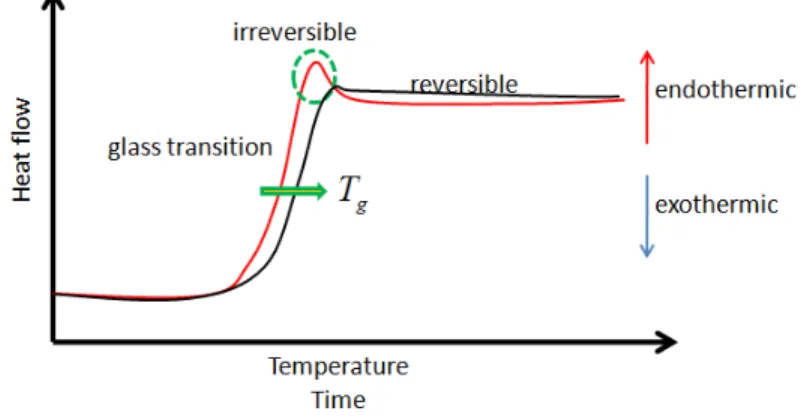
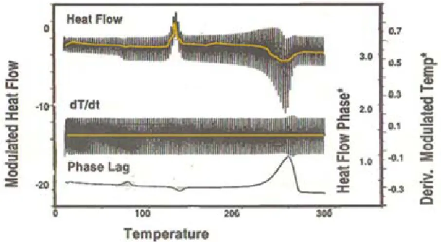
A sample MTDSC curve is given in Figure 2-6 where heat flow, heating rate and the phase between these signals is shown. A peak in the phase is an indication of irreversible processes.

Figure 2-6 Heating rate, heat flow and the phase lag graph of a MTDSC measurement. Average values of modulated heating rate and heat flow are highlighted. After [3].

The irreversible and reversible heat flow signals are deconvoluted by using MTDSC in Figure 2-7. Using the additional phase information obtained from

(27)

13 MTDSC it is possible to differentiate the two heat flow terms in Equation 2-5 as shown in the figure below.

Figure 2-7 The average reversible, irreversible and total heat flow signals of a MTDSC measurement are shown After [13].

2.2 Thermomechanical Analysis

Thermomechanical analysis (TMA) is the measurement of variations in sample dimensions, such as length or volume, as a function of temperature while a mechanical stress is applied. If the applied stress is removed and only effects of temperature are monitored on sample dimensions, the technique is called thermodilatometry. In this way thermal expansion coefficients can be determined and variations with respect to temperature and/or time are monitored. The technique determines the coefficient of thermal expansion coefficient of sample from the relationship [3, 4]

2.6 where is the thermal expansion coefficient, is the initial length, T is the temperature. Many materials deform under applied stress at a particular

(28)

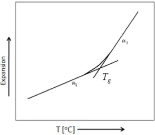
14 temperature which is often connected with the material melting or undergoing a glass-rubber transition [4]. Figure 2.8 shows a generic TMA curve; thermal expansion coefficient of a glassy material is different before and after the glass transition point.

Figure 2-8 A typical TMA curve for a glassy material indicating thermal expansion coefficient change around the Tg, glass transition, point.

2.3 Dynamic Mechanical Thermal Analysis

(DMTA)

DMTA is a method for investigating the morphology of materials which can be particularly sensitive to low energy transitions which are not readily observed by differential scanning calorimetry [9]. Many of these low energy transition processes are time-dependent, and by using a range of mechanical oscillation frequencies the kinetic nature of these processes can be investigated. DMTA can be performed either by applying a force initially and monitoring free oscillations while scanning sample temperature or, more frequently, by continuous application of oscillatory force while monitoring oscillations and scanning the temperature simultaneously [4].

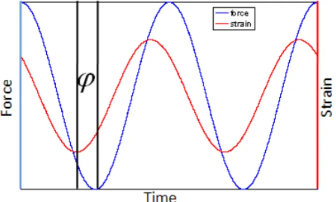
The most common DMTA measurement is simply measuring the Young modulus (E) and damping factor against a stepwise increased temperature while an oscillating force at frequency (ω). When the oscillating force

(29)

15 , 2.7 is applied to a system the strain response is given as

sin 2.8 where is the phase lag between the applied force and the strain response. The complex modulus is given as

2.9 where and are the maximum values of applied force and induced strain, respectively. The real part of corresponding to the storage modulus and the imaginary part of corresponding to the loss modulus are given as

| | , 2.10 | | . 2.11 The loss factor is a function of the phase between the applied force and induced strain as shown in Figure 2-9.

Figure 2-9 The phase relationship between applied force and induced strain for a dynamic mechanical test.

Real viscoelastic materials can be modeled as having the properties both of elasticity and viscosity. For example the Kelvin-Voigt model predicts that the material behavior can be represented by a purely viscous damper and purely elastic spring connected in parallel, whereas for a Maxwell material they are

(30)

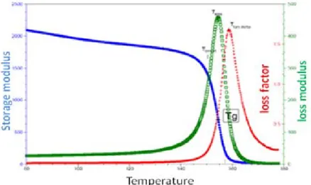
16 connected in series. However Maxwell model does not describe creep, and the Kelvin-Voigt model does not describe stress relaxation so a combination of the both models is developed known as the standard-linear material model [14]. In Figure 2.10 storage modulus, loss modulus and loss factor are drawn against temperature. Around the glass transition region, storage modulus decreases and a dramatic change in loss modulus and loss factor is observed.

Figure 2-10 Storage modulus, loss modulus and loss factor are shown for a glassy material with respect to temperature. Significant changes occur around glass transition temperature.

Gadaud et al determined the Young modulus and the damping factor of bulk glasses versus temperature using dynamical resonant and subresonant techniques [15-18]. The breakpoints of Young modulus (E) and damping factor ( ) versus temperature (T), and resonance frequency of the beam versus temperature (T) curves indicates the glass transition temperature. Figure 2.11 shows the data of the experiment conducted for GeAsSe glass [15].

(31)

17

Figure 2-11 (a) Modulus and damping coefficient of GeAsSe glass; (b) corresponding resonance frequency.

2.4 Micro / Nano Calorimeters

The conventional instrumentation for thermal analysis methods, described in the previous sections, enables the characterization of mainly bulk materials. On the other hand, the recent increasing trend towards micro and nano scale systems has brought about the extensive use of small scale materials whose physical properties differ considerably from bulk ones due to the large surface to volume ratio. These property changes include crystal structure changes [19, 20]; melting temperature decreases with respect to bulk values [21-23]; stress relaxation depends on the material size [24-26]. Therefore, to meet the need for the characterization of nanoscale material properties various micro/nano scale thermal sensors that are based on conventional thermo analytical methods have been developed.

For conventional calorimeters, the energy required to heat the calorimetric cell itself (the addenda) would be large compared to either the energy required to heat the sample or the energy involved in the transformation of the sample for samples of small scale. So, the signal of interest would be masked by the contribution from the addenda [27]. Thus, techniques and sensors that are more

(32)

18 sensitive are required. One of the obvious ways to increase the sensitivity is to make the calorimetric cell as small as possible, thus minimizing the effect of addenda.

The developing field of microelectromechanical systems (MEMS) enables the fabrication of ever-small size cell comparable with the size of the sample. Therefore, creation of new characterization probes for the study of material behavior at small scales becomes possible by MEMS technology. By using this technology, various types of calorimetric probes for materials of small scale have been developed [8, 21, 27-38].

L. H. Allen from the University of Illinois at Urbana-Champaign fabricated nanocalorimeters of scanning and differential scanning types and used them for characterization of various small scale materials. The technique used are same as the conventional calorimetry however, by introducing MEMS technology, they decreased the size of calorimetric cells increasing sensitivity that allows small scale calorimetric measurements such as heat capacity, latent heat, transition temperature determination [21, 27-34].

Various other groups used the same technique and similar instrument designs. Vlassak et al demonstrated parallel nano-DSC for combinatorial analysis of nanoscale materials. In this method signal is simultaneously collected from an array of calorimetric cells which is principally based on Allen’s design [35]. A novel approach by Gimzewski and Güntherodt is to use the deflection of a bimetallic microcantilever upon heating. For example they measured the phase transition temperatures of n-alkanes placed on the cantilever and associated enthalpy changes with a resolution of 10 nJ [36-38].

2.5 Micro-Thermal Analysis

Micro-Thermal Analysis combines the imaging capabilities of atomic force microscopy (AFM) with localized thermal analysis which is able to measure thermal transitions on a small area of a few square microns. The technique has a

(33)

19 variety of measurement modes, enabling two or more simultaneous measurements [39].

For these analyses, a conventional AFM tip is replaced with a cantilever having a miniature heater/thermometer on it. The cantilever, when used in conjunction with a reference probe, can be used as an ultra-miniature differential scanning calorimeter. Although the total sample is large in comparison to the sensor, probe heats and measures a very small area, a few square microns [40]. Thus monitoring the differential DC power that changes the probe temperature; monitoring the differential AC power and phase gives information about thermodynamic properties of sample resembling DSC and MTDSC results. Since the probe is mounted on the microscope stage, its deflection in the z-axis can be monitored during the experiment. This is the microscopic equivalent of the TMA method. Moreover, with this probe DTMA can be conducted if the cantilever is driven by an oscillatory force while the amplitude and phase of the oscillatory movement of the cantilever are monitored [39,40]

Micro/nano calorimeters that have been developed so far are used to determine heat capacity, thermal transitions and associated enthalpies of small scale materials down to picoliter volumes and nanogram mass. There are various types of micro/nanocalorimeters which are available as commercial products [41]. Although available micro/nano calorimeters are reasonably good for measuring thermodynamic properties, they are not integrated with other thermal methods.

Characterization of thermomechanical properties simultaneously with thermodynamical properties is not possible with available micro/nano calorimetry. Separate analysis should be conducted for different properties which is time consuming. In the micro-thermal analysis case, performing various types of measurements simultaneously is possible; however obtaining quantitative information is not possible due to uncertain sample mass. Moreover, heating a very small localized region in a bulk material does not mean nanoscale effects are readily observable.

(34)

20 In the next chapter an analytical model will be developed for a micro thermal analysis probe whose operation principles are based on scanning calorimetry, thermomechanical analysis (TMA), and dynamic mechanical thermal analysis (DMTA).This probe enables thermomechanical and thermodynamical analysis of picoliter volume materials.

(35)

21

Chapter 3 Modeling of System Behavior

The goal of this chapter is to build an analytical model starting from input voltage for obtaining a cantilever deflection formula. The thermal probe described in this thesis is an electrothermally driven bilayer microcantilever which becomes three-layer upon sample placement on it. Applied voltage on the electrical terminals of the cantilever that has finite resistance, reveals power and induces a temperature rise on the cantilever. Induced temperature rise, forces the cantilever to deflect due to thermal expansion coefficient mismatches between constituent layers. This means that energy is converted between three energy domains: (1) electrical domain, (2) thermal domain, and (3) mechanical domain. For the understanding of the cantilever behavior, interaction between these domains should be analyzed. Figure 3.1 shows the system-model-representation that illustrates how energy domains interact.

Figure 3-1 System Model Representation of the Cantilever

As Figure 3-1 reveals, combined electrothermal and thermomechanical analysis is necessary for the characterization of the device behavior. Due to easiness of the analysis, circuit-model of the system for each energy domain will be used throughout this chapter [42]. Section 3.1 develops electro-thermal analysis,

(36)

CHAPTER 3. MODELING OF SYSTEM BEHAVIOR

22 Section 3.2 describes mechanical behavior of the cantilever for AC and DC heat loading cases and lastly Section 3.3 describes the overall electro-thermo-elastic behavior of the device for combined DC and AC voltage application.

3.1 Electro-thermal analysis

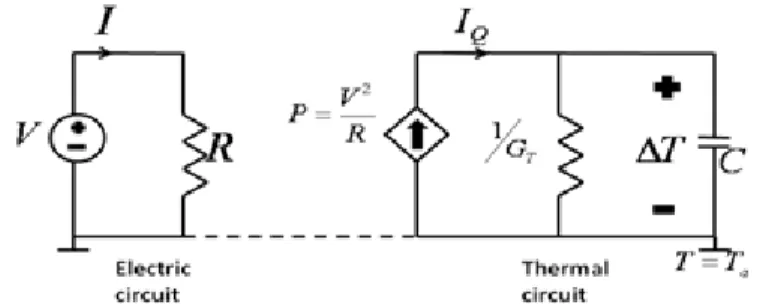
Joule-heating is the process by which the passage of electrical current through a resistive element releases heat inducing temperature rise on the element. This process can be modeled with the aid of the lumped-element thermal circuit of Figure 3.2 [42, 43].

Figure 3-2 Circuit model for the self-heating of a resistor driven from a voltage source.

Consider that the cantilever is initially at ambient temperature Ta, upon heating

of cantilever with the voltage generated power

, 3.1

cantilever temperature T increases. Solution of the electric-circuit representation of the thermal model yields the differential equation below, where ∆T (T-Ta) is

the difference between instantaneous and initial temperature of the cantilever:

Δ 3.2

where C is the total heat capacity and GT is the total thermal conductance of the

cantilever. Heat capacity is material and geometry dependent and given by the formula below for a rectangular m-layer cantilever width of b and length of L where ρi, ci, and hi are density, specific heat and thickness of the ith layer

(37)

23

… 3.3

Three heat exchange mechanism determine the thermal conductance of the cantilever: (1) Heat conduction between the cantilever and substrate which is assumed ideally at ambient temperature through cantilever materials, (2) heat-exchange between the cantilever and environment by thermal radiation, and (3) heat-exchange between the cantilever and environment by convection. Hence, GT is the sum of conductive thermal conductance GC, radiative thermal

conductance GR and conductance due to convection Gcv [45]:

3.4

GC and GR are given as

… , 3.5

4 . 3.6

where ki, εi are thermal conductivity and emissivity of ith layer material and σ is

the Stefan-Boltzman constant (5.67 x 10-8 W/m2K).

For analysis of thermal conductance due to air convection Grashof (GrL) and

Reynold (ReL) are defined as [46]

, 3.7

. 3.8

where g, β, T, Ta, L, ν, ρ, u∞ and μ are the gravitational constant, volumetric

CTE, temperature of the cantilever, temperature of the heat sink (i.e. substrate), length between the membrane and the heat sink, kinematic viscosity, mass density, mass average fluid viscosity and viscosity, respectively. For 1 natural convection may be neglected.

(38)

24 Figure 3.3 illustrates how temperature increases respectively with the driven voltage for specific material properties given in table 3.1 where convection is neglected. Temperature increases quadratically with applied DC voltage.

Material CTE, α (10-6 K-1₎ E(Gpa) k (W/K.m) c (J/kg.K) ρ (Kg/m3₎ Si 2.6 162 149 700 2420 Au 14.3 80 318 130 19400 GAST 14.4 21.9 0.2 130-150 4880

Table 3-1Material Properties

Figure 3-3 Temperature of the Si/Au bilayer cantilever versus applied dc voltage

3.1.1 Thermal Frequency Response upon AC

Heating

If the equation 3.2 is solved in frequency domain:

1 ∆ 3.9

The thermal transfer function can be calculated as ∆ 3.10 0 5 10 15 0 200 400 600 800 1000 Tem p er atur e (C ) Voltage

(39)

25 τ is the thermal time constant of the cantilever and given as . The thermal time constant τ can also be defined as the point where amplitude of the response decreases to 0.707 of its initial value and τ can be obtained from frequency response shown in figure 3.4 experimentally.

Figure 3-4 Thermal frequency response of the cantilever: Amplitude and phase of the thermal transfer function.

3.2 Thermo-elastic Analysis

Thermoelastic analysis describes the relation between the electrothermal power and cantilever deflection.

3.2.1 Thermal Deflection of Multilayer

Structures

A multilayer structure will deflect due to thermal expansion coefficient mismatches of constituent layers when temperature variations occur. In order to obtain a relation between the temperature change and induced deflection, we can decompose the structure to individual layers and apply an effective force Fi and

an effective moment Mi to each layer with the sign convention as illustrated in

Figure 3-5. 102 103 104 105 0 5000 10000 A m pl it ude ( a .u .) Driving Frequency (Hz) 102 103 104 105 250 300 350 400 P h a se (d eg ree) Driving Frequency (Hz)

(40)

26

Figure 3-5 One-end-fixed and one-end-free m-layer structure. All layers have same length, L along.

When the static equilibrium is reached all forces and moments should sum up to zero by conservation laws.

… 0 3.11

∑ 0

3.12 From beam theory,

1 3.13

where Ei, hi are the Young modulus and thickness of ith layer respectively, b is

width, and r is the radius of curvature of the beam. Total strains at layer boundaries should be equal, resulting in a set of (m-1) equations:

∆ ∆ 1 1 3.14

where

(41)

27 is the temperature induced strain;

, 3.16

is the effective force induced strain;

, 3.17

is the moment induced strain and has negative signs at the top and bottom of each layer. The radius of curvature r can be obtained by solving Equation 3.12, Equation 3.13 and m-1 equations obtained in equation 3.14 simultaneously. Assuming the tip deflection at the free-end of the structure (δ) is small compared to its length L, and then it can be expressed in terms of r as

∆ . 3.18

Since the thermal probing cantilever consists of two-layer and upon placing a sample on it, it becomes three-layer structure; bilayer and three-layer cantilever deflection equations are given. The general equations for m-layer are simplified for bilayer case is given as below [46]

∆ 3.19

Urey et al gives the analytical solution for the deflection of a three-layer structure assuming that middle layer is much thicker than the bottom and top

layers( ) as below [47]

3 3 ∆ 3.20

Figure 3.6 shows deflection vs. temperature curves for bilayer and three-layer structures for material properties tabulated in table 3.1.

(42)

28

Figure 3-6 DC deflection vs. Temperature and DC deflection vs. DC voltage.

3.2.2 Cantilever Dynamics

The thermal probe is a bilayer cantilever, its one end is clamped to substrate and other end is free. The electrical circuit equivalent of the mechanical system is shown in Figure 3-7. When it is driven with an external force, it can be simply modeled as a damped driven harmonic oscillator and satisfies the nonhomegenous second order linear differential equation

sin . 3.21

Here, x is the vertical deflection, m is the mass of the cantilever, β is the velocity-dependent damping constant, and k is the spring constant. The solution to Equation 3.21 is

sin . 3.22

where A is the amplitude and φ is the phase of the oscillation. Both of them are frequency-dependent and are given as

0 200 400 600 800 1000 0 2 4x 10 -6 D C de fl e c ti on (m ) Temperature (C) 0 5 10 15 0 2 4x 10 -6 D C de fl e c ti on(m ) Voltage

(43)

29 /

/ , 3.23

. 3.24

Figure 3-7 Electrical Circuit Representation of The Cantilever as damped, driven harmonic oscillator.

Phase has the opposite signs for and cases. Here, is the first harmonic resonance frequency of the cantilever, and is the Q-factor. The maximum amplitude occurs at driving frequency ωmax and

they are given by

/

/ / , 3.25

1 . 3.26

The mechanical transfer function relating x to F is given as /

3.27

Figure 3.8 shows the mechanical frequency response of a cantilever having resonance frequency of 39.4 KHz and quality factor of 40.

(44)

30

Figure 3-8 Mechanical frequency response of the cantilever: amplitude and phase.

3.2.3 Thermomechanical Response upon AC

Heating

If oscillatory heating electrothermal power is applied to the cantilever, the amplitude and phase of the oscillatory deflection of the cantilever can be formalized using the equations

, , , ∆ 3.28

where , is a function of variables relating temperature difference to this difference induced force which drives the cantilever. For bilayer cantilever D is given as

3.29

and for three layer cantilever it is given as

3 3 3.30 101 102 103 104 105 0 100 200 A m p li tude ( m ) Driving Frequency (Hz) 101 102 103 104 105 100 200 300 400 P h as e ( d e g re e) Driving Frequency (Hz)

(45)

31 since interaction relation between thermal and mechanical energy domains is formalized, the circuit model representation of the total thermomechanical behavior of the system is given as in Figure 3-9.

Figure 3-9 The circuit model representation of the thermomechanical system.

Frequency-domain solution of the circuit yields thermomechanical transfer function:

3.31

Figure 3-10 shows the thermomechanical frequency response of the cantilever which is a combination of thermal and mechanical frequency responses.

Figure 3-10 Thermomechanical frequency response of the cantilever: amplitude and phase. 102 103 104 105 0 2 4 6x 10 4 A m pl it ud e ( a .u ) Driving Frequency (Hz) 102 103 104 105 0 200 400 P h a s e ( d eg ree) Driving Frequency (Hz)

(46)

32

3.3 Overall Electro-Thermomechanical Analysis

When combined DC and small signal AC voltage is applied to the cantilever, a small oscillatory deflection superimposed on DC deflection occurs. Application of a voltage

cos 3.32

produces power of

3.33

when, there is no sample placed on the cantilever (in the assumption of constituent materials are stable in the given temperature range), temperature and DC deflection of the cantilever induced by the DC component of the power is shown in Figure 3-11.

Figure 3-11Temperature and Deflection vs. Voltage of bilayer cantilever.

Figure 3.12 shows the amplitude and phase of the oscillation at frequency ω when vs. Vdc when V is applied.

(47)

33

Figure 3-12 Amplitude and Phase of the thermomechanical oscillation at ω vs. Vdc.

If the third layer material placed on the cantilever that has a glass transition (See Figures 3-13a and 3-13b) in the reached temperature range, temperature dependencies of specific heat and Young modulus are formulized by equations below for analytical solutions described in the previous sections. Their variations with temperature are illustrated in Figure 3-15. Figures 3-16 to 3-19 show cantilever response based on this formulization.

Δ . 3.34

Δ . 3.35

E3 , Tg, and c3 are Young modulus, glass transition temperature and specific heat

of the sample respectively, where i and f subscripts stand for initial and final values of E3 and c3 before and after glass transition. ΔE3 and Δc3 are differences

between initial and final values of E3 and c3 respectively and delT defines the

glass transition temperature range.

0 5 10 15 0 0.5 1 1.5x 10 -10 A m p lit u d e ( m ) Voltage 0 5 10 15 -200 -100 0 P h a se ( d eg ree) Voltage

(48)

CHAPTER Fig tem tem Fig tem In Figure change o defined in cantilever of the osc thermal tr shown in factor shi R 3. MODE gure 3-13 a) Yo mperature b) He mperature. gure 3-14 Spec mperature range e 3.15, varia f sample la n Figure 3.1 r is excited t illation incre ransition eve Figure 3-12 ft results in 0 0 200 400 600 c(J/ kg .K ) 0 1 1.5 2 2.5x 10 E( Pa ) ELING OF S oung modulus eat capacity vs

ific heat and Y e modeled by e ation in res ayer during 5 based on thermomech eases linearl ents since m 2. During th n deviation f 200 T 200 010 T YSTEM BE vs. temperatur s. temperature i Young modulus eq. 3.20 and 3. onance freq glass trans measureme hanically at i ly with the in materials visc hermal trans

from this lin

400 60 Temperature 400 60 Temperature EHAVIOR re in the range in the range of s variation in th 21. quency is du sition. Qual nts from lite its resonanc ncreasing vo coelastic pro ition, resona near behavi 00 800 e(C) 00 800 e(C) of glass transit f glass transitio he glass transit due to Youn lity factor v erature [15] e frequency oltage in the operties do ance frequen or and decr 1000 1000 34 tion on tion ng modulus variation is . When the y, amplitude e absence of not alter as ncy and Q-rease in the

(49)

35 amplitude and shift in the phase of cantilever vibration driven at its initial resonance frequency thermomechanically as shown in figure 3-17.

Figure 3-15 Resonance Freq and Quality Factor of Cantilever vs. Temperature.

Figure 3-16 Temperature and DC deflection vs. Vdc.in the presence of glass transition.

If the deflection vs. Vdc graphs in Figures 3-11 and 3-16 are compared,

difference between two graphs is observed. Deflection graph in Figure 3-11

0 200 400 600 800 1000 3.5573 3.5574 3.5575 3.5576x 10 4 R e s ona nc e F re q( H z ) Temperature(C) 0 200 400 600 800 1000 20 30 40 Q u ali ty F acto r Temperature(C) 0 5 10 15 0 500 1000 T e m p er atu re ( C ) Voltage 0 5 10 15 -1 -0.5 0 x 10-6 D e fl ecti o n (m ) Voltage

(50)

36 increases quadratically with Vdc, where the one in Figure 3-16 deviates from this

quadratic behavior due to variation in elastic modulus of the material. There is no obvious difference between two temperature graphs since the addenda (8.65×10-8J/K) of the cantilever is large compared to sample heat capacity (3.96×10-9_J/K).

Figure 3-17 Amplitude and phase of thermomechanical oscillation at ω0 vs. Vdc.

If Figure 3-12 and Figure 3-17 are compared in the same manner the deviation from linear behavior of the amplitude is seen which is due to a variation in elastic modulus of the material. Moreover, in the presenece of glass transition a slight decrease in phase occurs which is not seen in Figure 3-12.

If AC voltage is removed and cantilever is driven at its initial resonance frequency mechanically by oscillatory force of 1nN and heated with application of Vdc simultaneously, the amplitude and phase of the oscillation will be in

Figure 3-18. In the absence of thermal transition, amplitude and phase would be constant since resonance frequency and Q-factor are constant. Variation of frequency and Q results in decrease of phase and amplitude of mechanical oscillation driven at initial resonance frequency of the cantilever.

Amplitude and phase of vibrations at two different frequencies in the range of resonance frequency for the same excitation force yield exact information about variations in resonance frequency and Q-factor of the cantilever with

0 5 10 15 0 2 4 6x 10 -10 A m pl it ude ( m ) Voltage 0 5 10 15 -178.4 -178.2 -178 -177.8 P h a se (d eg re e ) Voltage

(51)

37 temperature. Solution of equations below gives the resonance frequency and quality factor. Ri, φi are amplitude and phase of the vibrations driven at

frequency ωdi respectively. F is the mechanical driving force, k is the spring

contant that varies also with temperature, and ω0 is the resonance frequency.

1 3.36

3.37

Figure 3-18 Amplitude and phase of oscillation at ω0 driven mechanically vs. Vdc

In summary, this chapter presented analytical electrothermomechanical modeling of two/three layer microcantilever. Starting from applied voltage, heating of the cantilever, DC deflection upon heating, thermal, mechanical and thermomechanical responses are analyzed. Effects of variations in material properties namely young modulus, heat capacity and internal loss on the cantilever behavior are analyzed for comparison with the experimental results presented in the following chapter.

0 5 10 15 2 3 4 5x 10 -9 Am p li tu d e ( m ) Voltage 0 5 10 15 -90.2 -90.1 -90 -89.9 P h ase ( d eg ree) Voltage

(52)

38

Chapter 4 Device Fabrication, Measurements

and Results

In this chapter, firstly fabrication steps for two similar bilayer microcantilever thermal probes are presented. Then, these probes were used for the thermal analysis of thin film chalcogenide glasses As2S3 and Ge-As-Se-Te. The thermal

excitation and optical measurement setups to detect mechanical deflection and oscillation of the probes are described. Finally, measured deflection, amplitude and phase of the oscillations are presented. In the light of analytical method developed in the previous chapters the observed thermomechanical events are discussed.

4.1 Device Fabrication

Two analogous bilayer microcantilevers thermal probes are used for the thermomechanical analysis. The first type is the SiNX/Ni bilayer

microcantilevers. Hundreds of these microcantilevers, with various dimensions but same geometry, were fabricated on a single chip at the Advanced Research Laboratory, Bilkent University. With these cantilevers, thermomechanical actuation was demonstrated in principle. Although thermal analysis measurements could not be performed with these cantilevers, they still can be used as thermal actuators. The second type of the microcantilevers used is a commercial resistive AFM cantilever of Park Scientific Instruments. This second type is modified by ion beam milling to be used for thermal sensing purposes at the Institute of Materials Science and Nanotechnology, Bilkent University.

(53)

CHAPTER 4. DEVICE FABRICATION, MEASUREMENTS, AND RESULTS

39

4.1.1 SiN

x

/Ni Cantilever Probe Fabrication

The first type SiNx/ Ni bilayer cantilevers are fabricated using conventional bulk

micromachining technology. SiNx and Ni are selected as device materials since

they are stable for a vast temperature range and are chemically inert. They are well-known materials in micromachining technology and provide fabrication convenience; fabrication of large arrays of devices is straightforward. Moreover, the large thermal resistance coefficient (TCR) of Ni makes it a good candidate for use as resistive layer since large TCR is advantageous for temperature probing by monitoring resistance variation.

The fabrication of the probe involves the steps of conventional bulk micromachining as shown in Figure 4-1 and are briefly described below.

Wafer cleaning is an essential step for removal of dirt and dust on substrates that may decrease the quality of the films deposited on the substrate thus corrupting device operation. Wafer cleaning was performed by rinsing the wafer with acetone then with isopropyl alcohol (IPA).

Next step is the SiNx Growth process. 900 nm SiNx film is deposited on

110-oriented Si substrate by plasma enhanced chemical vapor deposition (PECVD) system at chamber temperature of 250°C. During the film deposition, SiH4 and

NH3 gas flows are stabilized to 180 sccm and 22.5 sccm respectively, resulting

10 nm/min film growth rate. This process induces residual stresses in the SiNx

(54)

CHAPTER 4. DEVICE FABRICATION, MEASUREMENTS, AND RESULTS

40

Figure 4-1 SiNx/Ni bilayer cantilever fabrication steps involves conventional bulk micromachining.

Patterning of SiNx; AZ 5214E positive resist is spin-coated on the SiNx film at

5200 rpm for 40 seconds and soft-baked at 110 °_{C for 60 seconds.}

Photolitography step is performed with Karl SussTM MA-6 mask aligner under 4 mW, 350 nm uv-light illumination for 60 seconds. Mask is turned 45° along the substrate normal for releasing the devices in KOH solution in the following steps of the fabrication process. Illuminated areas of the photoresist are removed by 4:1 DI water/AZ® 400K developer solution. Photoresist is hard-baked at 110

°_{C for 2 minutes for a better adhesion during etching process. Then, unmasked}

regions of SiNx are removed by wet etching by keeping the sample in 1:50

HF/DI water solution for 90 seconds. The resulting patterned SiNx film is shown

in Figure 4-2. After the etching process masking photoresist layer is removed by rinsing with acetone.

Micro and nanostructured devices for thermal analysis

MICRO AND NANOSTRUCTURED DEVICES

FOR THERMAL ANALYSIS

A THESIS

SUBMITTED TO THE PROGRAM OF MATERIALS SCIENCE AND

NANOTECHNOLOGY

AND THE INSTITUTE OF ENGINEERING AND SCIENCES

OF BILKENT UNIVERSITY

IN PARTIAL FULLFILMENT OF THE REQUIREMENTS

FOR THE DEGREE OF

MASTER OF SCIENCE

By

Özlem Şenlik

September, 2008

ABSTRACT

MICRO AND NANOSTRUCTURED DEVICES FOR

THERMAL ANALYSIS

ÖZET

TERMAL ANALİZLER İÇİN MİKRO VE NANO YAPILI

AYGITLAR

Acknowledgements

Table of Contents

List of Figures

List of Tables

Chapter 1

Introduction

Chapter 2

Theoretical Background

2.1 Calorimetry

2.1.1 Differential Scanning Calorimetry (DSC)

2.1.2 Temperature Modulated DSC

2.2 Thermomechanical Analysis

2.3 Dynamic Mechanical Thermal Analysis

(DMTA)

2.4 Micro / Nano Calorimeters

2.5 Micro-Thermal Analysis

Chapter 3

Modeling of System Behavior

3.1 Electro-thermal analysis

3.1.1 Thermal Frequency Response upon AC

Heating

3.2 Thermo-elastic Analysis

3.2.1 Thermal Deflection of Multilayer

Structures

3.2.2 Cantilever Dynamics

3.2.3 Thermomechanical Response upon AC

Heating

3.3 Overall Electro-Thermomechanical Analysis

Chapter 4

Device Fabrication, Measurements

and Results

4.1 Device Fabrication

4.1.1 SiN

/Ni Cantilever Probe Fabrication