A dynamic system approach for solving nonlinear programming problems with exact penalty function

(1)

See discussions, stats, and author profiles for this publication at: https://www.researchgate.net/publication/228654944

A dynamic system approach for solving nonlinear programming problems

with exact penalty function

Conference Paper · January 2008

CITATION

1

READS

95

2 authors:

Some of the authors of this publication are also working on these related projects:

Special Issue - New Methods and Techniques to Describe the Dynamics of Biological ApplicationsView project

ICAME’18: International Conference on Applied Mathematics in EngineeringView project Fırat Evirgen Balikesir University 31PUBLICATIONS 82CITATIONS SEE PROFILE Necati Ozdemir Balikesir University 75PUBLICATIONS 643CITATIONS SEE PROFILE

(2)

20th EURO Mini Conference

“Continuous Optimization and Knowledge-Based Technologies” (EurOPT-2008)

May 20–23, 2008, Neringa, LITHUANIA

L. Sakalauskas, G.W. Weber and E. K. Zavadskas (Eds.): EUROPT-2008 Selected papers. Vilnius, 2008, pp. 82–86

A DYNAMIC SYSTEM APPROACH FOR SOLVING NONLINEAR PROGRAMMING PROBLEMS WITH EXACT PENALTY FUNCTION

Necati Özdemir1_{and Fırat Evirgen}

Department of Mathematics, Faculty of Science and Art, Balıkesir University, Cagis Campus, Balıkesir 10145, Turkey

E-mail: nozdemir@balikesir.edu.tr, fevirgen@balikesir.edu.tr

Abstract: The Dynamic system has attracted increasing attention in recent years. In this paper, a dynamic system approach for solving Nonlinear Programming (NLP) problems with inequality constrained is pre-sented. First, the system of differential equations based on exact penalty function is constructed. Further-more, it is found that the equilibrium point of the dynamic system is converge to an optimal solution of the original optimization problem and is asymptotically stable in the sense of Lyapunov. Moreover, the Euler scheme is used for solving differential equations system. Finally, two practical examples are illust-rated the effectiveness of the proposed dynamic system formulation.

Keywords: nonlinear programming, exact penalty function, dynamic system, lyapunov function. 1. Introduction

Nonlinear Programming (NLP) problems are commonly encountered in modern science and technol-ogy. Most of efficient methods have been developed for solving NLP problems. The method of penalty function has the attractive tool to solve the problems of NLP for many years. More extensive knowledge about them can be found in (Luenberger, 1973) and (Sun, 2006). Also differential equation methods are an alternative approach to solution of these problems. In this type of methods an optimization problem is formulated as a system of ordinary differential equations (ODEs) so that the equilibrium point of this sys-tem converges to the local minimum of the original problem.

The methods based on ODE for solving optimization problems have been proposed by Arrow and Hurwicz (Arrow, 1956), Fiacco and Mccormick (Fiacco, 1968) and Evtushenko (Evtushenko, 1994). However, Brown and Biggs (Brown, 1989) and Schropp (Schropp, 2000) were shown that ODE based methods for constrained optimization can be perform better than some conventional methods. Recently, Wang (Wang et al., 2003) and Jin (Jin, 2007) have prepared a differential equation approach for solving NLP problems.

In this paper, we presented a differential equation approach for solving inequality-constrained opti-mization problems. This approach shows that the stable equilibrium point of the dynamic system is also an optimal solution of the corresponding optimization problem.

The rest of paper is organized as follow three sections. In Section 2, we will construct a dynamic sys-tem model based on exact penalty function (Meng et al., 2004b). Moreover, we will prove that the syssys-tem can converge to the optimal solution of the constrained optimization problem and discuss the stability of equilibrium point. A Lyapunov function is set up during the procedure. In Section 3, two illustrative ex-amples will be given to emphasize the effectiveness of the proposed system. In Section 4, conclusions will be given.

2. A New Dynamic System Approach

Let us consider the following nonlinear programming problem m i x gfi(x) 0 ,12,3,..., subject tominimize ( )≤ = (1) 1_{Corresponding Author}

(3)

A DYNAMIC SYSTEM APPROACH FOR SOLVING NONLINEAR PROGRAMMING PROBLEMS WITH EXACT PENALTY FUNCTION

where x=

(

x1,x2,...,xn

)

T∈Rn, f R R

n_→

: _and_g =

(

_g₁_,_g₂_,...,_g_m

)

T_:_Rn→_Rm

(

_m≤_n

)

_{. The functions}

f and g are assumed to be convex and twice continuously differentiable. The objective penalty function

of (1) is defined as

(

)

∑

= + + − = m i gi x M x f M x F 1 2 2 ₍ ₎ ) ( ) , ( (2) whereF_:Rn_×R_→R

, M ∈R and gi+(x)=max

{

0,gi(x)

}

, i= ,12,...,m. Therefore, the unconstrained

optimization problem is define as follows

). , ( minimize_n R x M x F ∈ (3)

The objective penalty function has been investigated by Meng in the reference (Meng et al., 2004b). The

authors proved that the objective penalty function F( Mx, ) _{is exact if there is some}_M*_{such that an}

op-timal solution of (3) is also an opop-timal solution of (1) for any given M ≥M*. Furthermore, they

intro-duced a neural network for solving NLP problems based on exact penalty function, see Liu and Meng (Liu, 2003a).

By straightforward calculation, the gradient and Hessian matrix of exact penalty function are given as, respectively

(

)

(

)

(

( )

)

( ) 2 ( ) ( ) 2 ( ) ( .) 2 ) ( ) ( 2 ) , ( ) ( 2 ) , ( ) ( ) ( 2 ) ( ) ( 2 ) , ( 1 2 1 2 2 1

∑

= + = = + ∇ + ∇ ∇ + ∇ − + ∇ ∇ = ∇ − − = ∇ ∇ + ∇ − = ∇ m i i xx i m i T i x i x xx T x x xx M m i i x i x x x g x g x g x g x f M x f x f x f M x F M x f M x F x g x g x f M x f M x F

In order to solve the unconstrained optimization problem (3), the new dynamic system is defined by the following system of differential equations

(

)

∑

= + _∇ − ∇ − − = m i i x i xf x g x g x M x f dt dx 1 ( ) ( ) 2 ) ( ) ( 2 (4a)

(

( )

)

. 2 f x M dt dM ₌ ₋ _(4b)

Definition 1 A point (x*,M*)_{is called an equilibrium point of (4) if it satisfies the right hand side of the}

equations (4a) and (4b).

In here, we are going to prove that the equilibrium point of the corresponding dynamic system (4) is equivalent to the optimal solution of the problem (3) and vice versa.

Theorem 1 If (x*,M*)_{is the equilibrium point of the dynamic system (4), then}x*_{is an optimal solution}

to the unconstrained optimization problem (3).

Proof Since (x*,M*)_{is the equilibrium point of the dynamic system (4), we have}

(

( )

)

( ) 2 ( ) ( ) 0 2 1 * * * * * * = ∇ − ∇ − − =

_∑

= + m i i x i xf x g x g x M x f dt dx ₍₅₎

(

( )

)

0. 2 * * * = − = f x M dt dM ₍₆₎

So clearly first order necessary condition is satisfied. To obtain the second order sufficient optimality condition we have to show that the Hessian matrix of the exact penalty function is positive definite. From the equations (5) and (6), we get

0 ) ( ) ( 1 * * _∇ ₌

∑

= + m i gi x xgi x and ( ) . * * _M x f = (7)

Consequently, using the equations (7) the Hessian matrix is positive definite and so x*_{is the optimal}

(4)

Theorem 2 If x* is the optimal solution to the unconstrained optimization problem (3) for the penalty

parameter M*, then (x*,M*)_{is the equilibrium point of the dynamic system (4).}

Proof According to the assumption, first order necessary condition is hold. That is 0 ) , ( * * = ∇_xF x M _or * ₌0. dt dx (8)

Furthermore, in (Meng et al., 2004b), it is shown that x* is also a feasible solution for the problem (1). It

means gi+(x)=max

{

0,gi(x)

}

=0. From the equation (8) and the feasibility of x*, we can say that

0 *

= dt dM

. Thus (x*,M*)_{is the equilibrium point of the dynamic system (4).}

2.1. Stability Analysis

Now, it will be discussed the stability of the dynamic system (4). Necessary definitions and theorems for the Lyapunov stability theorem can be found in the references (La Salle, 1961) and (Curtain, 1977).

Definition 2 Let Ω be an neighbourhood of (x*,M*)_{. A continuously differentiable function V is said}

to be a Lyapunov function at the state (x*,M*)_{for dynamic system (4) if satisfy the following}

condi-tions:

a) V( Mx, )_{is equal to zero for the equilibrium point}₍x*_,M*₎_,

b) V( Mx, )_{is positive definite over Ω some neighbourhood of}₍x*_,M*₎_,

c) dV_dt is semi-negative definite over Ω some neighbourhood of (x*,M*)_.

It is well known that the equilibrium point (x*,M*)_{is not only stable for a Lyapunov function which is}

satisfies above conditions, but also it is asymptotically stable if there exists a Lyapunov function V

satis-fies _<0

dt dV

in some neighbourhood Ω .

Now we define a suitable Lyapunov function for dynamic system (4) corresponding to the exact pen-alty function as follows

(

( )

)

( ) . ) , ( ) , ( 1 2 2

_∑

= + + − = = m i gi x M x f M x F M x V

Theorem 3 If (x*,M*)_{is an equilibrium point of the dynamic system (4), then}₍x*_,M*₎_is

asymptoti-cally stable for (4).

Proof It is clear that from assumption and optimality conditions, first two conditions are provided.

More-over, by the derivative of V( Mx, )_{with respect to t , we have}

T T M V x V M V x V dt dM dt dx M V x V dt dM M V dt dx x V dt dV     ∂ ∂ − ∂ ∂ −     ∂ ∂ ∂ ∂ =         ∂ ∂ ∂ ∂ = ∂ ∂ + ∂ ∂ = 2 2_<0.             ∂ ∂ +       ∂ ∂ − = M V x V

As a result, (x*,M*)_{is asymptotically stable for the dynamic system (4).}

3. Illustrative Examples

(5)

A DYNAMIC SYSTEM APPROACH FOR SOLVING NONLINEAR PROGRAMMING PROBLEMS WITH EXACT PENALTY FUNCTION . 0 25 4 ) ( subject to 7 7 5 . 0 ) ( minimize 2 2 2 1 2 1 2 1 2 2 2 1 ≤ − + = − − − + = x x x g x x x x x x x f

The optimal solution is x* ₌

( )

2,3T and the optimal value of the objective function f(x*)₌₋30. For

solving above problem, we convert it to an unconstrained optimization problem with exact penalty func-tion (2)

(

0.5 7 7

)

max

{

0 ,4 25

}

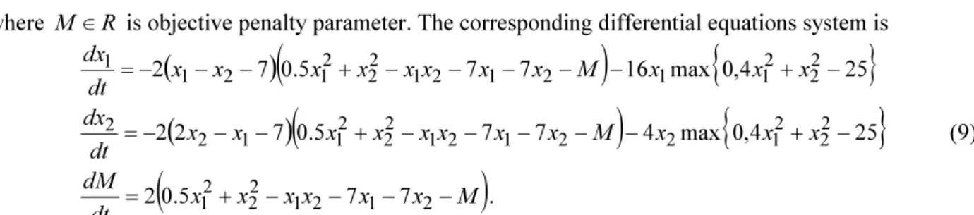
, ) , (x M = x12+x22−x1x2− x1− x2−M 2+ x12+x22− 2 F

where M ∈R is objective penalty parameter. The corresponding differential equations system is

(

)

(

)

{

}

(

)

(

)

{

}

(

0.5 7 7

)

. 2 25 4 , 0 max 4 7 7 5 . 0 7 2 2 25 4 , 0 max 16 7 7 5 . 0 7 2 2 1 2 1 2 2 2 1 2 2 2 1 2 2 1 2 1 2 2 2 1 1 2 2 2 2 2 1 1 2 1 2 1 2 2 2 1 2 1 1 M x x x x x x dt dM x x x M x x x x x x x x dt dx x x x M x x x x x x x x dt dx − − − − + = − + − − − − − + − − − = − + − − − − − + − − − = (9)

The Euler method is used to solve the differential equations system (9) with initial points

( )

,1−1 ,

( )

−11, ,

( )

2 −, 2 ,

(

−2,2

)

and M0=−100 with step size ∇t =0.0001, simulation result shows the trajectory of

dy-namic system converges to its optimal solution in the Fig. 1.

-2 -1 0 1 2 3 4 -2 -1 0 1 2 3 4 x1 x2 0 2 4 6 1 2 3 4 t x1 0 2 4 6 -1 0 1 2 3 4 t x2

Fig. 1. Optimal solution for Example 1 with different initial points Example 2 Consider the following nonlinear programming problem (Schittkowski, 1987)

( )

(

)

. 0 25 . 0 ) ( subject to 1 100 ) ( minimize 2 2 2 1 2 1 2 2 1 2 ≤ − − = − + − = x x x g x x x x f

The optimal solution of this problem is x* ₌

( )

11,T and the optimal value of the objective function

0 )

(x* =

f . Similar calculation as in Example 1, we have below objective penalty function (2) with

objec-tive penalty parameter M ∈R,

( )

(

1

)

max

{

0 ,0.25

}

. 100 ) , ( 12 22 2 2 2 1 2 2 1 2 x x M x x x M x F  + − −      ₋ ₊ ₋ ₋ =

The corresponding differential equations system is

( )

(

)

(

) ( )

( )

{

}

( ) ( )

( )

{

}

( )

1 . 100 2 25 . 0 , 0 max 4 1 100 400 25 . 0 , 0 max 4 1 100 1 4 800 2 2 2 1 2 2 2 2 1 2 2 2 2 1 2 2 1 2 2 2 2 2 1 1 2 2 2 1 2 1 2 1 2 1 1       ₋ ₊ ₋ ₋ = − − +       ₋ ₊ ₋ ₋ − − = − − +       ₋ ₊ ₋ ₋ − + − = M x x x dt dM x x x M x x x x x dt dx x x x M x x x x x x x dt dx (10)

(6)

86

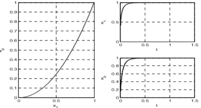
The differential equations system (10) is solved by using the Euler method. If we choose the initial values

for x1(0)=0, x₂(0)=0 and M0=−20 with step size ∇t =0.00005, simulation result gives the

trajec-tory of dynamic system converges to its optimal solution in the Fig. 2.

0 0.5 1 0 0.1 0.2 0.3 0.4 0.5 0.6 0.7 0.8 0.9 1 x₁ x 2 0 0.5 1 1.5 0 0.5 1 t x 1 0 0.5 1 1.5 0 0.2 0.4 0.6 0.8 1 t x 2

Fig. 2. Optimal solution for Example 2 with _M₀₌₋20 4. Conclusions

We have considered a dynamic system approach for solving NLP problems (1) with inequality con-strained in this work. Dynamic system model (4) has been constructed based on exact penalty function method (Meng et al., 2004). Through theoretical analysis and example computations, it has been shown that the equilibrium point of the dynamic system (4) can reach to the optimal solution of the NLP problem (1). In addition, the equilibrium point of the system was proved to be asymptotically stable in the sense of Lyapunov stability theorem. Hence, the simulation result illustrate that this approach is applicable.

References

Arrow, K. J. and Hurwicz, L. 1956. Reduction of constrained maxima to saddle point problems, in J. Neyman (ed.), Proceedings of the 3rd_{Berkeley Symposium on Mathematical Statistics and Probability, University of} Califor-nia Press, Berkeley, 1–26.

Brown, A. A. and Bartholomew-Biggs, M. C. 1989. ODE versus SQP methods for constrained optimization, Jour-nal of Optimization Theory and Applications 62(3): 371–385.

Curtain, R. F. and Pritchard, A. J. 1977. Functional Analysis in Modern Applied Mathematics. Academic Press, London.

Evtushenko, Yu. G and Zhadan, V. G. 1994. Stable barrier-projection and barrier-newton methods in nonlinear pro-gramming, Optimization Methods and Software 3(1–3): 237–256.

Fiacco, A. V and Mccormick, G. P. 1968. Nonlinear Programming: Sequential Unconstrained Minimization Tech-niques. John Wiley, New York.

Hock, W. and Schittkowski, K. 1981. Test Examples for Nonlinear Programming Codes. Springer, Berlin.

Jin, L.; Zhang, L-W. and Xiao, X. T. 2007. Two differential equation systems for inequality constrained optimiza-tion, Applied Mathematics and Computation 188(2): 1334–1343.

La Salle, J. and Lefschetz, S. 1961. Stability by Liapunov’s Direct Method with Application. Academic Press, Lon-don.

Liu, S. and Meng, Z. 2003a. A new nonlinear neural networks based on exact penalty function with two-parameter, in Proceeding of the Second International Conference on Machine Learning and Cybernetics 2(2–5): 1249– 1254.

Luenberger, D. G. 1973. Introduction to Linear and Nonlinear Programming. Addison Wesley, Reading, Massa-chusetts.

Meng, Z., et al. 2004b. An objective penalty function method for nonlinear programming, Applied Mathematics Letters 17(6): 683–689.

Schittkowski, K. 1987. More Test Examples For Nonlinear Programming Codes. Springer, Berlin.

Schropp, J. 2000. A dynamical systems approach to constrained minimization, Numerical Functional Analysis and Optimization 21(3–4): 537–551.

Sun, W. and Yuan, Y.-X. 2006. Optimization Theory and Methods: Nonlinear Programming. Springer, New York. Wang, S.; Yang, X. Q. and Teo, K. L. 2003. A unified gradient flow approach to constrained nonlinear optimization