Experiments with two-stage iterative solvers and preconditioned Krylov subspace methods on nearly completely decomposable Markov chains

EXPERIM EN TS W ITH TWG-STVVGE ITE R A TIV E

SOIA/HERS AND P R E eb N P IT IO N E ^

SUBSPAGE M ETH OD S ON NEARLY COM PLETELY

DECOM POSABLE M ARK O V CHAINS

A THESIS

SUBMITTED TO THE DEPARTMENT OF COMPUTER

ENGINEERING AND INFORMATION SCIENCE

AND THE INSTITUTE OF ENGINEERING AND SCIENCE

OF BILKENT UNIVERSITY

IN PARTIAL FULFILLMENT OF THE REQUIREMENTS

FOR THE DEGREE OF

MASTER OF SCIENCE

By

W ail

G ueaieb

Ju n e , 1997

SUBSPACE METHODS ON NEARLY COMPLETELY

DECOMPOSABLE MARKOV CHAINS

A THESIS

SUBMITTED TO THE DEPARTMENT OF COMPUTER ENGINEERING AND INFORMATION SCIENCE

a n d t h e INSTITUTE OF ENGINEERING AND SCIENCE OF BILKENT UNIVERSITY

IN PARTIAL FULFILLMENT OF THE REQUIREMENTS FOR THE DEGREE OF

MASTER OF SCIENCE

By

Wail Gueaieb

June, 1997

I certify that I have read this thesis and that in my opin­ ion it is fully adequate, in scope and in quality, as a thesis for the degree of Master of Science.

' -wx!

I----Asst. Prof. Dr. Tuğrul Dayar(Principal Advisor)

I certify that I have read this thesis and that in my opin­ ion it is fully adequate, in scope and in quality, as a thesis for the degree of Master of Science.

Assoc. Profi Dr. Cevdet Aykanat

I certify that I have read this thesis and that in my opin­ ion it is fully adequate, in scope and in quality, cis a thesis for the degree of Master of Science.

yJ u\

\jj''---Asst. PiW. tor) Mustafa Ç. Pınar

Approved for the Institute of Engineering and Science:

ABSTRACT

EXPERIMENTS WITH TWO-STAGE ITERATIVE SOLVERS AND PRECONDITIONED KRYLOV SUBSPACE METHODS ON NEARLY

COMPLETELY DECOMPOSABLE M ARKOV CHAINS

Wail Gueaieb

M.S. in Computer Engineering and Information Science Supervisor: Assistant Professor Dr. Tuğrul Dayar

.June, 1997

Preconditioned Krylov subspace methods are state-of-the-art iterative solvers developed mostly in the last fifteen years that may be used, among other things, to solve for the stationary distribution of Markov chains. Assuming Markov chains of interest are irreducible, the ¡problem amounts to computing a pos­ itive solution vector to a homogeneous system of linear algebraic equations with a singular coefficient matrix under a normalization constraint. That is, the (n X 1) unknown stationary vector x in

A x = 0, ||a:||^ = 1 (0.1)

is sought. Here A = I — , an n x n singular M-matrix, and P is the one-step stochastic transition probability matrix.

Albeit the recent advances, practicing performance analysts still widely pre­ fer iterative methods based on splittings when they want to compare the per­ formance of newly devised algorithms against existing ones, or when they need candidate solvers to evaluate the performance of a system model at hand. In fact, experimental results with Krylov subspace methods on Markov chains, especially the ill-conditioned nearly completely decomposable (NCD) ones, are few. We believe there is room for research in this area siDecifically to help us understand the effect of the degree of coupling of NCD Markov chains and their nonzero structure on the convergence characteristics and space requirements of preconditioned Krylov subspace methods.

The work of several researchers have raised important and interesting ques­ tions that led to research in another, yet related direction. These questions are the following: “How must one go about partitioning the global coefficient matrix A in equation (0.1) into blocks if the system is NCD and a two-stage iterative solver (such as block successive overrelaxation— SOR) is to be em­ ployed? Are block partitionings dictated by the NCD normal form of F neces­ sarily superior to others? Is it worth investing alternative partitionings? Better yet, for a fixed labelling and partitioning of the states, how does the perfor­ mance of block SOR (or even that of point SOR) compare to the performance of the iterative aggregation-disaggregation (lA D ) algorithm? Finally, is there any merit in using two-stage iterative solvers when preconditioned Krylov subspace methods are available?”

Experimental results show that in most of the test cases two-stage iterative solvers are superior to Krylov subspace methods with the chosen precondition­ ers, on NCD Markov chains. For two-stage iterative solvers, there are cases in which a straightforward partitioning of the coefficient matrix gives a faster solution than can be obtained using the NCD normal form.

Key words: Markov chains, near complete decomposability, stationary iter­ ative methods, projection methods, block iterative methods, preconditioning, ill-conditioning.

İKİ SEVİYELİ DOLAYLI ÇÖZÜCÜLER VE İYİLEŞTİRİLMİŞ KRYLOV ALTUZAY YÖNTEMLERİ İLE NEREDEYSE BÖLÜNEBİLİR MARKOV

ZİNCİRLERİ ÜZERİNDE DENEYLER

Wail Gueaieb

Bilgisayar ve Enformcitik Mühendisliği, Yüksek Lisans Tez Yöneticisi: Yrd. Doç. Dr. Tuğrul Dayar

Haziran, 1997

İyileştirilmiş Krylov altuzay yöntemleri çoğunlukla son onbeş yılda geliş­ tirilmiş, başka şeyler yanında, Markov zincirlerinin durağan dağılımlarını elde etmede kullanman en son dolaylı çözücülerdir. İlgilenilen Markov zincirlerinin indirgenemez olduğu varsayılırsa, problem tekil bir katsayı matrisine sahip bir türdeş lineer cebirsel denklemler takımına bir normalleştirme şartı altında po­ zitif bir çözüm vektörü hesaplamaktan ibarettir. Yani,

A x = 0, ||.t||i = 1 (0.1) deki (n X l ) ’lik bilinmeyen durağan vektör x aranmaktadır. Burada A - I - P '^

n X n tekil bir M-matrisi ve P bir-adımhk rassal geçiş olasılık matrisidir.

Son gelişmelere rağmen, mesleklerini icra eden başarım çözümleyicileri, yeni tasarlanmış algoritmaların başarımını var olanlarla kıyaslamak istediklerinde, veya eldeki bir sistem modelinin başarımını değerlendirmek için aday çözücülere gerek duyduklarında, hala çoğunlukla bölmeye dayanan dolaylı yöntemleri ter­ cih etmektedirler. Esasında, Markov zincirleri, özellikle de hastalıklı neredeyse bölünebilir olanları üzerinde Krylov altuzay yöntemleri ile deneysel sonuçlar pek azdır. Biz bu alanda, özellikle de neredeyse bölünebilir Markov zincir­ lerinin bağlanma derecelerinin ve sıfırdan farklı yapılarının iyileştirilmiş Krylov altuzay yöntemlerinin yakınsama özellikleri ve yer gerekleri üzerindeki etkilerini anlamamıza yardım edecek araştırmalar için yer olduğuna inanıyoruz.

Bazı araştırmacıların çalışmaları başka fakat ilintili yönde araştırmaları ne­ den olan önemli ve ilginç sorular ortaya çıkardı. Bu sorular şunlardır: “Eğer

sistem neredeyse bölünebilirse ve (blok ardcırda üst yumuşatma— SOR gibi) iki seviyeli bir dolaylı çözücü kullanılacaksa, (0.1) denklemindeki global kat­ sayı matrisi A ’yı nasıl parçalara ayırmalı? P ’nin neredeyse bölünebilir normal yapısının zorunlu kıldığı blok ayrıştırmalar diğerlerine oranla mutlaka daha mı üstündür? Alternatif ayrıştırmalara yatırım yapmaya değer mi? Hatta, durum­ lar sabit adlandırılıp ayrıştırıldığında blok ardarda üst yumuşatmanın (hatta nokta ardarda üst yumuşatmanın) başarımı dolaylı birleştirme-ayrıştırma al­ goritmasının başarımı ile nasıl kıyaslar? Son olarak, iyileştirilmiş Krylov al- tuzay yöntemleri varken iki seviyeli dolaylı çözücüleri kullanmanın bir değeri var mıdır?”

Deneysel sonuçlar pek çok test vakasında iki seviyeli dolaylı çözücülerin seçilmiş iyileştiriciler için Krylov altuzay yöntemlerine göre neredeyse bölünebi­ lir Markov zincirlerinden daha üstün olduklarını göstermektedir. İki seviyeli dolaylı çözücüler için, katsayı matrisinin basit bir ayrıştırılmasının neredeyse bölünebilir yapısının kullanılarak bulunacak bir tcineden daha hızlı çözüm ver­ diği vakalar vardır.

Anahtar kelimeler. Markov zincirleri, neredeyse bölünebilirlik, durağan do­ laylı yöntemler, projeksiyon yöntemleri, blok dolaylı yöntemler, iyileştirme, hastalıklılık.

A C K N O W L E D G M E N T S

I would like to thank Dr. Tuğrul Dayar for his invaluable help, time, persistent encouragement, advice, ideas and suggestions throughout this study. He was the one to introduce me to the area, and he not only has been a role model but also more than a friend. Without his continuing support and supervision, this work would not have been possible. Special thanks cire due to Dr. Aykanat and Dr. Pınar for the time they provided to read and review this thesis and for their keen acceptance to be in my committee. I also would like to extend my gratitude to the professors I have taken courses with and I have got to know during the past six years. I especially would like to acknowledge Dr. Ulusoy, Dr. Flenner, Dr. Güvenir, Dr. Kerimov cind Dr. Dikovsky from whom I have learned a lot. They will greatly influence my future work.

I am grateful to the graduate administration of the Department of Com­ puter Engineering and Information Science for the financial support provided throughout my graduate studies at Bilkent University and to the faculty and staff of the same department for creating a pleasant environment for learning and research.

I also would like to thank all my friends here for their friendship and con­ tinuous support.

Lastly, I am forever grateful to my parents, brothers and sister for their unwavering support throughout my student life.

1 Introduction and Overview

1.1 Markov Chains

1.1.1 Definitions

1.1.2 Discrete and Continuous Time Markov C h a in s... 2

1.1.3 Probability Distributions

1.1.4 Numerical P rop erties... 7

1.2 State Classification

1.2.1 Definitions 10

1.2.2 Following P r o p e r t ie s ... 11

1.3 Decomposable Probability M citrices... 14

1.4 NCD Markov C h a in s ... 16

2 Numerical Solution Methods 18

2.1 Direct Methods 19

2.2 Iterative M e th o d s... 21

2.2.1 SOR: A Stationary Iterative M e t h o d ... 22

2.2.2 Block Iterative M e t h o d s ... 26

2.2.3 Projection M eth od s... 34

2.2.4 Stopping C r ite r ia ... 47

2.2.5 P recon dition ers... 49

2.3 ImiDlementation Considerations 53 3 M odels Used 57 3.1 Complete Buffer Sharing With Pushout Thresholds in ATM Net­ works ... 57

3.2 A Two-Dimensional Markov Clnun Model 61 3.3 An NCD Queueing Network of the Central Server T y p e ... 62

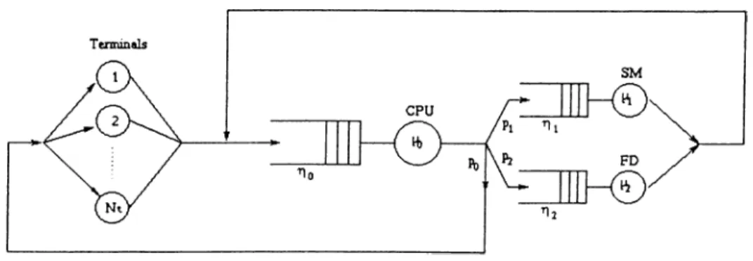
3.4 A Telecommunication M o d e l... 66

3.5 A Queueing Network with Blocking find Priority Service Model 69 3.6 A Multiplexing Model of a Leaky Bucket in Tandem ... 71

3.7 Mutex— A Resource Sharing M o d e l ... 72

4 Numerical Results 76 4.1 The Effect of Ill-C on d ition in g ... 82

4.2 The Effect of R eord erin g... 84

5 Conclusion and Future Work 86

A Tables of Results 88

3.1 A Two-Dimensional Markov Chain Model Model...62

3.2 An NCD Queueing Network of the Central Server Type Model. . 64

3.3 Telecommunication Model... 67

3.4 An ATM Queueing Network Model... 70

3.5 A Resource Sharing Model (Mutex). 74

2.1 Summary of Operations and Storage Requirements for SOR. . . 25

2.2 Summary of Operations and Storage Requirements for Block SOR at iteration k... 29

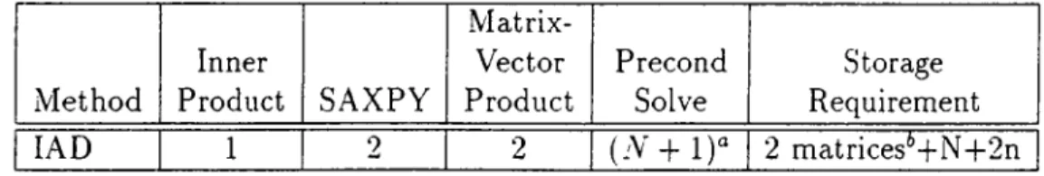
2.3 Summary of Operations and Storage Requirements for lAD at

iteration k. 33

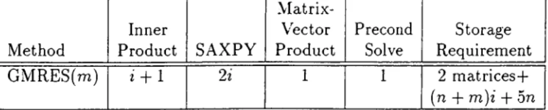
2.4 Summary of Operations and Storage Requirements for GMRES(?n) at iteration i ... 38

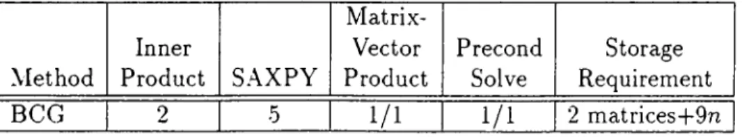
2.5 Summary of Operations and Storage Requirements for BCG at iteration i. “a/6 ” means “a” operations with the rncitrix and “ 6”

with its transpose. 41

2.6 Summary of Operations and Storage Requirements for CGS at

iteration i ... 43

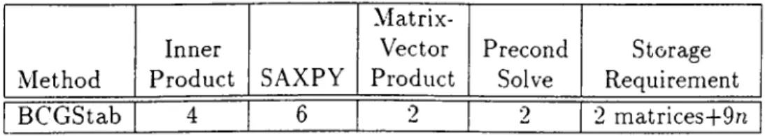
2.7 Summary of Operations and Stoi'cige Requirements for BCGStab

cit iteration i ... 43

2.8 Preconditioners used in the QM R versions... 45

2.9 Summary of Operations and Storage Requirements lor QMR at

iteration i ... 45

3.1 Characteristics of the Pushout Threshold Problem. 60

3.2 Partitioning Results for the easy Test Case. 60

3.3 Partitioning Results for the medium Test Case. 60

3.4 Partitioning Results for the hard Test Case. 61

3.5 Lower and Higher Bandwidths of the Pushout Threshold Test Matrices... 61

3.6 Characteristics of the Two-Dimensional Markov Chain Problem. 62

3.7 Partitioning Results for the Two-Dimensional Markov Chain Problem... 63

3.8 Lower and Higher Bandwidths of the Two-Dimensional Markov Chain Test Matrices... 63

3.9 Characteristics of the NCD Queueing Network Problem. 65

3.10 Partitioning Results for the ncd Test Case... 65

3.11 Partitioning Results for the ncd.altl Test Case. 66

3.12 Partitioning Results for the ncd^alt2Tesi Case. 66

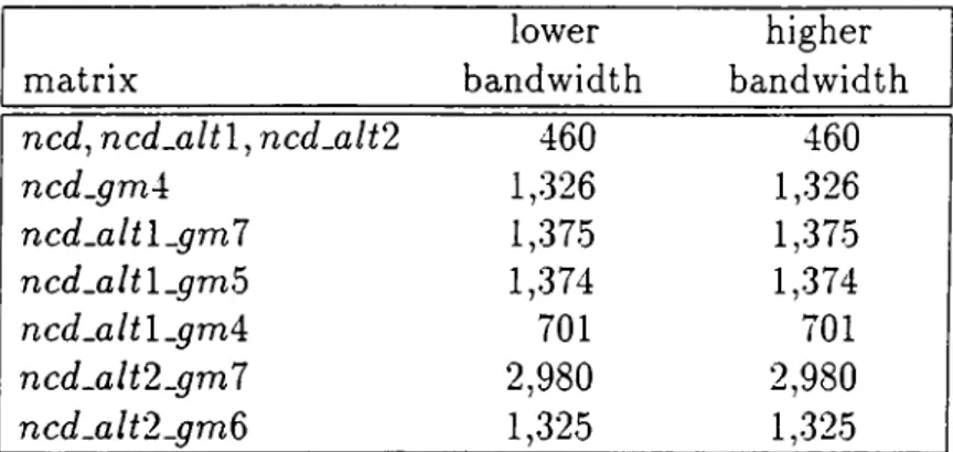
3.13 Lower and Higher Bandwidths of the NCD Queueing Network Test Matrices... 67

3.14 Characteristics of the telecom Problem... 68

3.15 Partitioning Results for the telecom Problem. 69

3.16 Lower and Higher Bandwidths of the Telecom Test Matrices. . . 69

3.17 Chax'acteristics of the ATM Queueing Network Problem. 71

3.18 Partitioning Results for the ATM Queueing Network Problem. . 71

3.19 Lower and Higher Bandwidths of the ATM Queueing Network Test Matrices... 71

3.21 Partitioning Results for the Leaky-Bucket Problem... 73

3.22 Lower and Higher Bandwidths of the leaky Test Matrix... 73

3.23 Characteristics of the Mutex Problem. 74

3.24 Partitioning Results for the mutex Test Matrix... 75

3.25 Partitioning Results for the mutex^altl Test Matrix... 75

3.26 Partitioning Results for the mutex_alt2 Test Matrix... 75

3.27 Lower and Higher Bandwidths of the Mutex Problem Test Ma­

trices. 75

Introduction and Overview

1.1

Markov Chains

1.1.1 Definitions

Understanding the behavior of physical systems is often achieved by modeling the system as a set of states which it can occupy and determining how it moves from one state to another in time. If the future evolution of the system does not depend on the past history but only on the current state, the system may be represented by a stochastic process. Stochastic processes arise extensively throughout queueing network analysis, computer systems performance evalu­ ation, large scale economic modeling, biological, physical, and social sciences, engineering, and other areas.

A stochastic process is a family of random variables { X { t ) , t € T } defined on a given probability space and indexed by the parameter i, where t varies over some index set (parameter space) T [36]. T is a subset of { —oo, + o o ) and is usually thought of as the time parameter set. X ( t ) denotes the observation at time t. If the index set is discrete, e.g., T = { 0 , 1 , . . . } , then we have a discrete (-time) stochastic process; otherwise, if T is continuous, e.g., T = {t : 0 < if < d-oo}, we call the process a continuous (-time) stochastic process. The values assumed by the random variable X { t ) are called states. The set of all

possible states represent the state space S of the process. This state space may be discrete or continuous.

A Markov process is a stochastic process whose next state depends on the current state only, and not on the previous states. By this, it is said to satisfy the “Markov property.” When the transitions out of state X { t ) depend on the time i, the Markov process is said to be nonhomogeneous. However, if the state transitions are independent of time, the Markov process is said to be homogeneous. If the state space of a Markov process is discrete, the Markov process is referred to cis a Markov chain. Throughout this work, we concentrate on discrete-time Markov chains (DTMCs) and continuous-time Markov chains (CTMCs) with finite state space.

To satisfy the Markov property, the time spent in a state of a Markov chain must satisfy the memoryless property: At any time i, the remaining time the chain will spend in its current state must be independent of the time already spent in that state. This means that this time must be exponentially distributed for CTMCs and geometrically distributed for DTMCs. These are the only distributions that possess the memoryless property.

1.1.2

Discrete and Continuous Time Markov Chains

In this section, we will provide formal definitions of DTMCs and CTMCs.

For a DTM C, is usually represented by Xn (n =; 0 ,1 ,. ..) as we observe the system at a discrete set of times. {X „ , n = 0 , 1 , . . . } is called a stochastic sequence. A DTMC satisfies the following relationship for all natural numbers n and all states x„.

Prob{Xn+i = Xn+ilXo = = x i , . . . , = x „ }

= Prob{X„.^i = x„+i|.Y„ = x „ }, n > 0. (1.1)

The conditional probabilities Prob{Xn+i = Xn+ilA"« = 3r„} are called the single-step transition probabilities, or just the transition probabilities, of the Markov chain.

For a time homogeneous DTMC, transition probabilities are independent of n, and hence may be written as

Pij = Prob{Xn+i = j\Xn = Vn = 0 ,1 --- and i j e S. (1.2) The matrix P whose i,;th element is given by p,j, for all i and j , is called the transition probability matrix, or the chain matrix [36]. P is a stochastic matrix, i.e., its elements pij satisfy the following two properties

0 ^ Pij ^ Ij V i , j 6 <5, (1-3)

= (1.4)

j

Let Xj(n) = Prob{Xn = i ) , Vj G S. Note that X)jg5 7rj(n) = 1. Then 7r(n) = (7Ti(n), 7T2(^)) · · · ? ^«(^)i · · ·) denotes the state probability vector at step n. Note that we shall adopt the convention that all probability vectors are row vectors. All other vectors will be considered to be column vectors unless specifically stated otherwise. The probability of being at a particular state j just after the nth transition may be expressed as

~ 1) PiA > 1· i'€5

Equation (1.5) can be rewritten in matrix form as

7r(n) = 7r(n — 1) P, n > 1.

(1.5)

(1.6)

Analogously, a CTMC may be described as

Prob{X{tn+i) = a:n+i|X(io) = ^OiNi{ti) = Xi, . . . , X{ t n) = Xn}

= Prob{X{tn+i) = Xn+i\X{trx) = Xn},

n >

0

.

(1.7)

For the transition probabilities, we write

Pij(sJ) = P r o b { X { t ) = j\X{s) = i}, t , s > 0 , i , j e S . (1.8) When the CTMC is homogeneous— and that is what we are interested in— these transition probabilities depend only on the difference A t = t ~ s , and not on s and t. So we can rewrite equation (1.8) as

For a better understanding of the relationship between CTMCs and DTMCs, consider the time axis as a sequence of mutually disjoint sufficiently small in­ tervals so that there is at most one transition in each subinterval. At the end of each A t time interval, there is exactly one transition, and hence the system behaves like a DTM C.

Let 'Kj{t -f- A t ) = P r o b { X { t -f- A t) = ji}, Vj G S. Note that + A t ) = 1. Then 7r(i -f A t ) denotes the state probability vector at time t A At.

We determine the probability of being in state j at time i -|- A i by

7Tj(i A t ) = ^ ^ ^ 0 ) Vj ^ S .

ies

This can be written in matrix form as

7r(i -I- A t ) = Tc{t) P { A t ) , t, A t > 0.

Here P { A t ) is the one-step transition probability matrix fo r the interval At whose ¿jth entry is given by p ,j(A i).

Let qij{t) be the rate at which transitions occur from state i to state j at time t. The transition rate is an instantaneous quantity that denotes the number of transitions that occur per unit time.

Um f o r . # j .

This leads to the following transition probability

Pij{t + A t ) = qij{t)At + o{At), for i ф j ,

where o (A i) is the '‘little oh” notation such that o{At) tends to 0 faster than A i.

,. o(At)

hm = 0.

д<—0 A i

Starting from the concept of probability conservation, we can write

1 - P i i { t , t + A t) = X ; p o ( i , i + A i)

Dividing by A t and taking the limit as At 0, we obtain quit) = lim ^ ^ ^ Ai '■ Hence, im < i—0 I pii{t,t + A t ) - 1 A t = limAi—0 A i / 9.-.(0 = - J 2 qij{t)· (1.9)

The matrix Q{t) whose ¿jth element is qij{t) is called the infinitesimal gen­ erator matrix, or transition rate matrix, for the CTMC. In matrix form, it

IS

where P { t , t + A i) is the transition probability matrix whose ijith element is

P i j { t , t + A t ) and I is the identity matrix. When the CTM C is homogeneous,

the transition rates qij are independent of time, and the transition matrix is simply written as Q.

The matrix Q has row sums of 0 as each of its diagonal elements is the negated sum of the corresponding off-diagonal elements (of that row). From equation (1.9) we get

qu — ~^^^qij· (1.10)

1.1.3

Probability Distributions

Determining the stationary distribution of a Markov chain is the core of this study. As defined in the previous section, for a DTMC, 7r,(n) denotes the probability that a Markov chain is in state i at step n, i.e.,

7T,(n) = Prob{Xn = *}, n > 0, i € <S.

D efin ition 1.1 (S ta tio n a ry d istrib u tion ) [36] Let P be the transition prob­ ability matrix o f a DTAIC, and let the vector z whose elements zj denote the probability o f being in state j be a probability distribution; i.e.,

Zj € IR, 0 < Zj < 1, and ^ zj = 1. j

D e fin itio n 1.2 (L im itin g d is trib u tio n ) [36] Given an initial probability dis­ tribution 7t(0), if the limit

lim ^(n), n—*-oo

exists, then the limit is called the limiting distribution, and we write 7T = lim 7r(n).

n—►OO ^

The limiting distribution is also known as the steady-state, or equilibrium, dis­ tribution. Informally speaking, the steady-state distribution is the probability distribution which, if it exists, the process will reach after sufficiently many transitions, independently of the initial probability distribution, and will re­ main in that distribution for all further transition steps. We will come back to this in later sections.

Now, taking the limit as n oo of both sides of equation (1.6), we obtain

7T = ttP, = IIttIIi = 1. (1.11)

i€S

Analogously to DTMCs, a stationary probability vector for a CTMC can be defined as any vector z such that zQ = 0, ||z||i = 1. The steady-state distribution of a CTMC, if it exists, is written as

7T = lim 7r(i)

and is independent of the initial probability distribution 7t(0). Recall that 7r,(i)

is the probability that a CTM C is in state i at time t, i.e..

x .(i) = P r o b { x { t ) = i}, Vi e <s.

Then,

7T,(i d- A f) = 7r,(i) f 1 - X ] <7.j(0^M + [ Y . 3ki

Since qa{t) = - 9>i(0j we have

{t)-Kk(t) A f A o{At).

and [ TTi{t + A t ) - o { At ) i ™ [ ---X t--- j = i n + A t / ’ i.e., d-iriit) dt = Y^<lki{,t)Trk{t). In matrix notation, this gives

dTr{t) dt

When the Markov chain is homogeneous, we may drop the time parameter t from the transition matrix Q and simply write

diT{t)

dt = Tr(i)Q.

If the limiting distribution tt exists, then after sufficiently long time t, 7r(t) w'ill converge to tt and dTr[t)/dt will be equal to 0. Hence, for a homogeneous CTM C,

^Q = 0, ^TT,· = ||7t||i = 1. ies

(1.1 2)

1.1.4

Numerical Properties

As we discussed in section (1.1.2), the transition matrix P is a stochastic matrix (see equations (1.3) and (1.4)). Besides, P is singular, and its order is equal to the cardinality of S. Note that equation (1.11) is an eigensystem in which the unit left-hand eigenvector of P , corresponding to the unit eigenvalue (= 1), is sought.

To proceed further, we need to introduce the definitions of the spectrum and the spectral radius of a matrix.

The spectrum of a matrix A is the set of all eigenvalues of A, and it is denoted by cr{A). In mathematical notation,

It is worth mentioning that the spectrum of a matrix A is equal to the spectrum of the transpose of A. In other words, cr(/l) = a{A^).

The spectral radius oi a matrix A is the largest eigenvalue of A, in magnitude, and it is denoted by p{A). In mathematical notation,

p{A) = rnax{|A|,A G cr(A)}.

One way of solving equation (1-11) is to transform it to a homogeneous linear system

x ( P - / ) = 0, ||7 r||i = l,

where tt is the unknown vector.

Unlike P , the infinitesimal generator matrix Q has row sums of 0 (see equa­ tion (1.10)). Equation (1-12) represents a homogeneous system of linear equa­ tions with Q as the coefficient matrix and tt as the unknown vector.

D e fin itio n 1.3 (M -m a tr ix ) [10] Tn ATmatrix A is any finite square ma­ trix with nonpositive off-diagonal elements and nonnegative diagonal elements which may be written in the form

A = r l - G , G > 0, r > p{G),

where r is a real scalar (r G IR), G is a square matrix, and I is the identity matrix.

The matrix —Q heis nonpositive off-diagonal elements. Let’s illustrate how —Q can be written in the form —Q = r l — G. Let G = r l A Q, where r = rnax,g5 |çü| > 0. The matrix ( l / r ) G is a stochastic matrix, hence p{G) < r. So all the conditions are satisfied and —Q is verified to be an M-matrix.

For determining the stationary distribution vector of a Markov chain, a DTM C formulation may be transformed to a CTMC formulation and vice versa.

D T M C = » C T M C : tt = ttP = > 0 = ttQ, where Q ^ P - I,

C T M C D T M C : 0 = kQ r = ttP, where P = {l/fi)Q + I and H =

1.2

State Classification

In order to be able to classify the states of a Markov chain, we need to introduce some new definitions. Without loss of generality, the following definitions will be valid for DTMCs only. However, it is easy to figure out the corresponding homogeneous CTMC definitions since we remarked the relationship between the two types.

Let be the probability of going from state i to state j in n steps. Then

= Prob{Xm+n = j

I Xm

I U = J

\ 0, if i ^ j

Now we are ready to introduce the Chapman-Kolrnogovov equation for Markov chains:

pS? = H p\k PkT‘^ for 0 < / < n. kes

In matri.x notation, it may be written as p(n) _ p(i)p{n-i)^

where is the matrix of n-step transition probabilities with entries p\j^ for all i i j G S. pVI is obtained by raising P to the nth power. In other words, p{n) _ pn

If the steady-state distribution tt of a DTMC exists, then

and hence

\imp\f=^TTj, V i J e S .

1.2.1

Definitions

Classifying states of Markov chains requires some definitions to be made, and we mainly follow [10] in that respect.

> State j is said to be accessible from state i if 3n > 0 for which > 0. > two states i and j are said to communicate if state i is accessible from

state j and state j is accessible from state i.

> A nonempty set C C is said to be closed if and only if Vi € C and Vj 0 C, j is not accessible from i.

> A Markov chain is said to be irreducible if all states communicate with each other.

> A state is said to be recurrent if the process, once in that state, returns to that state with probability 1. If the probability of returning to that state is strictly less than 1, then the state is said to be transient. Mathematically speaking, we can write

E p!.” = oo n = l oo E p! n = l

(n)

> A recurrent state i for which p„ = 1 is said to be an absorbing state. c> If the mean time to return to a state is finite, the state is said to be

positive recurrent, or recurrent nonnull. Otherwise, if the mean time to return to a state is infinite, given that the state is recurrent, then the state is said to be null recurrent.

> If all states of a Markov chain are positive recurrent, null recurrent, or transient, then we respectively have a positive recurrent, null re­ current, or transient Markov chain.

t> The period of state i, written d(i), is the greatest common divisor of all integers n > 1 for which > 0. If = 0 for all n > 1, then we define d{i) = 0.

> A Markov chain in which each state has period 1 is said to be aperiodic^ or acyclic; whereas, a Markov chain in which each state has the same periodicity and this period is greater than 1, is said to be periodic^ or cyclic.

> A positive recurrent, aperiodic state is said to be ergodic.

> If a Markov chain is irreducible, positive recurrent, and aperiodic, then it is said to be an ergodic Markov chain.

> A Markov chain with a finite state space S is said to be regular if

lim > 0.

n — ►CO

Hence, a steady-state distribution exists for a regular Markov chain. > A Markov chain with a finite state space is said to be doubly stochastic

Z] Pik = '^Pkj = V

yi,j e s.

kES k£S

1.2.2

Following Properties

In this section we will derive some important properties as a consequence of the definitions provided in the previous section.

• If two states communicate, then they are of the same type. That is, they are both either positive recurrent, null recurrent, or transient.

• States that communicate have the same periodicity.

• If the state space S is finite, then at least one of the states is positive recurrent.

• If the state space S is finite and the Markov chain is irreducible, then every state in S is positive recurrent.

• No state of a Markov chain with a finite state space can be null recurrent.

• If 7T is the stationary distribution for a Markov chain, then itj = 0 if state j is transient or null recurrent.

• If a Markov chain does not have any positive recurrent states, then the Markov chain does not have any stationary distribution. Besides, the state space of such a chain has to be infinite.

• Suppose 7T and ir' are two diiferent stationary distribution vectors for a Markov chain. Then there exists infinitely many stationary distribution vectors for the chain. In essence, any convex combination of tt and x' is also a stationary distribution for the Markov chain.

• Let C be any irreducible closed set of positive recurrent states in a Markov chain. Then there exists a unique stationary distribution tt for the chain that is concentrated on C. Stationary distribution probabilities for states outside C are all 0.

• Let S = St U Snr U Spr, be the state space of a Markov chain, where St is the set of transient states, S„r is the set of null recurrent states, and Spr is the set of positive recurrent states. The following is a summary regarding the stationary distributions of the chain:

> If Spr = 0, then there is no stationary distribution.

> If Spr ^ 0, then there is at least one stationary distribution.

> If Spr ^ 0, and Spr is irreducible and closed, then there is a unique stationary distribution concentrated on Spr·

> If Spr — OiCi and Cif)Cj = 0 for all i , j , then there is a unique station­ ary distribution vector tt,· concentrated on C, for all i. Furthermore,

7T= 5 ] Of,’Ti,

where a, > 0 for all i and X], a, = Í, is also a stationary distribution vector.

• Any irreducible, positive recurrent Markov chain ha^ a unique stationary distribution.

• If 7Г is a steady-state distribution for a Markov chain, then тг is the only stationary distribution.

• A regular Markov chain is irreducible, positive recurrent, and aperiodic.

• A steady-state distribution exists for an ergodic Markov chain.

One of the most important theorems in the domain of Markov chains is the Perron-Frobenius theorem. This theorem is very helpful because of its strong application to stochastic matrices (see [-36, 17]).

Theorem 1.4 (Perron-Frobenius) [36] Let .4 > 0 6e an irreducible square

matrix o f order n. Then,

1. » A has a positive real eigenvalue, Ax, such that Ax = p{A). • To p{A) there corresponds an eigenvector x > 0, i.e..

Ax = Axx and X > 0.

• p{A) increases when any entry o f A increases.

• p{A) is a simple eigenvalue o f A, i.e.. Ax is a simple root o f det{XI — Л) = 0.

2. Let S be a matrix o f complexed-valued elements and S* obtained from S by replacing each element by its modulus. If S* < A, then any eigenvalue p o f S satisfies

\p\ < Ax.

Furthermore, if for some p, j^ij = A x , then S*

p = A x e ' ^ , then

S = é^DAD~\

= A. More precisely, if

3, if A has exactly p eigenvalues equal in modulus to Ai^ then these numbers are all different mid are the roots of the equation

=

0

When plotted as points in the complex plane, this set o f eigenvalues is invariant under a rotation o f the plane through the angle 2Tr/p but not through smaller angles. When p > I then A can be symmetrically permuted

A = form 0 Ai2 0 0 ^ 0 0 A23 0 0 0 0 ·· Ap-i,p Ap\ 0 0 _{0 /}

in which the diagonal submatrices are square and the only nonzero submatrices are A 12, A 23, · · ·, Ap-\^p, Ap\.

1.3

Decomposable Probability Matrices

A special case of particular interest in Markov chains is when the chain is reducible. In such a case, the probability matrix may be transformed to a particular nonzero structure and is said to be decomposable [36].

D e fin itio n 1.5 (D e c o m p o s a b le M a trix ) A square matrix A is said to be decomposable if it can be brought by symmetric permutations o f its rows and columns to the form

A = U 0

W V

( U 3 )

where U and V are square nonzero matrices and W is, in general, rectangular.

If a Markov chain is reducible then there exists at least one ordering of the state space such that the probability matrix is in the form of (1.13). If U and

V are of orders nj and U2, respectively, where n { — rii + « 2) is the total number of states, then the state space may be decomposed to two disjoint sets

Hi = { s i , S2, . . . , i ! ni } , and H2 = {-Sni+l) · · · .-Sn})

where Sj’s {i = 1,2, . . . , n ) are the states of the Markov chain. For the time being, let’s suppose that VF ^ 0, i.e., there exists at least one nonzero entry in W . Observing the nonzero structure in (1.13), we can see that once the process is in one of the states of Bi, it can never pass to a state in B2· Consequently, Bi is known to be an isolated, or an essential set. On the other hand, being in one of the states of the set B2 guarantees staying in that set until the first transition to one of the states of Bi. Then set B2 is said to be transient, or nonessential. In the particular case where W = 0, the matrix is said to be completely decomposable. In this case, both Bi and B2 are isolated.

The matrix U may be decomposable, and hence can be permuted to the form in (1.13). If we continue in this pattern, the matrix A may be brought to a special form called the normal form of a decomposable nonnegative matrix, given by

A =

A l l 0 0 0 0 0

0 _A

22

0 0 0 Akk 0 0

Afc+l,! Afc+1,2 ... .■ · Ak+i,k 0

Am,l Arn,2 Am,k Am.k+l

\

/

. (1.14)

The diagonal blocks An (z = 1, . . . , m) are square nondecomposable matri­ ces. All the blocks to the left of the first k diagonal blocks (i.e.. An for i = 1 . 2 . . . . , k), and to the right of all diagonal blocks, are 0. For the submatrices to the left of the last m — k diagonal blocks (i.e., A.y for i = A: - ) - 1, . . . , m, j = 1 . . . . . 1 — 1), there exits at least one nonzero submatrix per row of blocks. Therefore, the diagonal blocks possess the following characteristics:

• An, i = k + I , . .. , m : transient, and again, nondecomposable.

This is quite logical and easy to figure out bearing in mind the nonzero structure of (1.14).

A probability matrix having the form in (1.14) according to the Perron- Frobenius theorem has a unique eigenvalue of multiplicity k. Besides, there exist k linearly independent left-hand eigenvectors corresponding to this unit eigenvalue. The last m — k entries of all these eigenvectors are all O’s as they correspond to transient states. Further details and proofs may be found in [36].

1.4

N C D Markov Chains

Consider a probability matrix having the form in (1-14). If we introduce “small” perturbations on some of the zero off-diagonal blocks to make them nonzeros (still conserving its stochastic properties (1.3) and (1.4)), the matrix is no longer decomposable and the Markov chain becomes irreducible. How­ ever, since the perturbations are small, meaning that the introduced nonzero entries have small values compared to those within the diagonal blocks, the matrix is said to be nearly decomposable. If, now, the nonzero elements in all the off-diagonal submatrices are small in magnitude compared with those in the diagonal blocks, then the matrix is said to be nearly completely decompos­ able (NCD). In NCD Markov chains, the interactions between the blocks is weak, whereas interactions among the states of each block are strong.

For an example, consider the following simple completely decomposable probability matrix:

P = 1.0 0.0 0.0 1.0

If we introduce small perturbations to the elements of P giving it the form

1.0 — Cl Cl P =

such that 1.0 — €i ^ and 1.0 — C2 >· C2, then the system becomes nearly completely decomposable.

Interestingly, NCD Markov chains arise frequently in many applications. It was noticed that a small perturbation in the matrix leads to a larger per­ turbation in the stationary distribution causing the computation of the sta­ tionary vector to be usually not as accurate as it is for ordinary irreducible Markov chains. Hence, NCD Markov chains are known to be ill-conditioned. Throughout this work, we are mainly concerned with NCD systems. We will come back to this in later chapters where we present different iterative solu­ tion techniques and compare and contrast their cornpetitivity in computing the stationary probability vector of finite NCD Markov chains.

Numerical Solution Methods

Many advanced scientific problems are practically impossible to solve analyti­ cally. As an alternative, numerical methods were introduced and they showed to be very efficient in solving a wide range of problems. We are interested in using numerical techniques to compute the stationary distribution vector of a finite irreducible Markov chain [2.3, 18, 9, 27, 21]. Our aim is to solve the homogeneous system of linear algebraic equations

A x = 0, ||i||, = 1, (

2

1

where A is a (n x n) singular, irreducible M-matrix [7] and x is the unknown (n X 1) positive vector to be determined. Since our problems stem from Markov

chain applications, the coefficient matrix A is taken as A = I — in case the one-step transition probability matrix is provided, or as A = —Q^ if we are supplied with the infinitesimal generator matrix. The solution vector x corresponds to (the transpose of the stationary distribution vector of the Markov chain). This explains the normalization constraint in equation (2.1) which also guarantees the uniqueness of the solution. The Perron-Frobenious theorem guarantees the existence of the solution since A is an M-matrix [7]. In the rest of this chapter we discuss the numerical techniques used to solve equation (2.1).

2.1

Direct Methods

Numerical methods that compute solutions of mathematical problems in a fixed number of floating-point operations are known as direct methods. The classical Gaussian elimination (GE) is a typical example of direct methods and it is suitable for irreducible Markov chains [36]. For a full (n x n) system of linear equations, the total number of operations required by GE is O(n^). The space complexity is O(n^). As it can be seen, these complexities grow rapidly with the problem size making GE (and direct methods in general) not suitable for large sparse matrices. Another problem with direct-solving methods is that the elimination of nonzero elements of the matrix during the reduction phase often results in the creation of several nonzero elements in positions that previously contained zero. This is called fill-in, and in addition to making the organization of a compact storage scheme more difficult (since provision must be made for the deletion and insertion of elements), the amount of fill-in can often be so extensive that available memory is quickly exhausted. Moreover, altering the form of the matrix may cause buildup of rounding errors [10].

It is known that if the coefficient matrix A is irreducible, there exist [24] lower and upper triangular matrices L and U such that

A = LU.

This LU decomposition is not unique. It is called the Doolittle decomposition if the diagonal elements of L are set to 1, and the Grout decomposition if the diagonal elements of U are set to 1. Usually, Gaussian elimination refers to the Doolittle decomposition.

Once an LU decomposition has been determined, a forward substitution step followed by a backward substitution is usually sufficient to determine the solution of the linear system. For example, suppose that we are required to solve A x = b where A is nonsingular, b ^ 0, and the decomposition of A = LU is available so that LU x = b. The idea is to set Ux = z, then the vector z may be obtained by forward substitution on Lz — b. Note that both L and 6 are known. The solution x may subsequently be obtained from Ux = z by backward substitution since by this time both U and 2 are known.

However, for homogeneous system of equations (i.e., 6 = 0) with a singular coefficient matrix, the last row of U (supposing that the Doolittle decompo­ sition is performed) is equal to zero. Proceeding as indicated above for the nonhomogeneous case, we get

Ax = LU X = 0.

If now we set Ux = z and attempt to solve Lz = 0. we end-up finding that 2 = 0 since L is nonsingular (d e t(i) = 1). Proceeding to the backward substitution on = 2 = 0 when = 0, we find that it is evident that may assume any nonzero value, say x„ = r¡. Hence, the remaining elements of x can be determined in terms of tj. The solution vector is then normalized if required. Note that for homogeneous linear systems the elimination is only needed to be carried out for the first n — 1 steps.

In the Doolittle decomposition L~^ exists and is called the multiplier matrix. L~^ is lower triangular and its ¿th column is composed of the multipliers that reduce the ith column below the main diagonal of .4 to zero to form the matrix U [36]. This phase is called the reduction phase.

Assume that U and L overwrite the upper triangular (including the diag­ onal) and the strictly lower triangular (excluding the diagonal) parts of A. Let A^^^ represent the altered coefficient matrix at the kth. step of the forward elimination. Then

W

a - — _o Hj ) i < k , Wj al; ' + P i k 0^kj i > k , ' i j where the multipliers are given by

(fc-l), (t-l) = -a ]k ¡H k ■ (k)

The elements are called the pivots and must be nonzero if the reduction is to terminate satisfactorily. For purposes of stability, it is generally necessary to interchange the rows of the matrix so that the pivotal element is the largest in modulus in its column in the unreduced portion of the matrix (called partial pivoting). This ensures that the absolute values of the multipliers do not exceed 1. For some cases, it is necessary to interchange both rows and columns so that the pivotal element is the largest among all elements in the unreduced part of

the matrix {full pivoting). However, for irreducible Markov chains no pivoting is necessary.

2.2

Iterative Methods

The term iterative methods refers to a wide range of techniques that use suc­ cessive approximations to obtain more accurate solutions to a linear system at each step. Iterative methods of one type or another are tire most com­ monly used methods for obtaining the stationary probability from either the stochastic transition probability matrix or from the infinitesimal generator. This choice is due to several reasons. First, in iterative methods, the only operations in which the matrices are involved are multiplications with one or more vectors. These operations conserve the form of the matrix. This may lead to considerable savings in memory required to solve the system especially when dealing with large sparse matrices. Besides, an iterative process may be terminated once a prespecified tolerance criterion has been satisfied, and this may be relatively lax. For instance, it may be wasteful to compute the solution of a mathematical model correct to full machine precision when the model itself contains error. However, a direct method is obligated to continue until the final operation has been carried out.

In this chapter we discuss three types of iterative methods: stationary iter­ ative methods, block iterative methods, and projection methods. Throughout our work we experimented with the (point) successive overrelaxation (SOR) method [.36, 4] as a stationary technique. Two types of block iterative methods were considered: block SOR and iterative aggregation-disaggregation (lA D ) [22, 33, 12]. As for projection techniques, we chose to implement and experiment with the methods of Generalized Minimum Residual (GMRES) [25, 30, 31], Bi­ conjugate Gradient (BCG) [15, 4], Conjugate Gradient Squared (CGS) [32, 37], Biconjugate Gradient Stabilized (BCGStab) [37], and Quasi-Minimal Residual (Q M R ) [13, 14]. SOR and the two block iterative methods we used are part of the Markov Chain Analyzer (MARC.A) [35] software package version 3.0.

2.2.1

S O R : A Stationary Iterative Method

Stationary iterative methods are iterative methods that can be expressed in the simple form [4]

or(^+i) = r:c(^) + c, k = 0 A , . . . (2.2) where neither T nor c depend upon the iteration count k. Equation (2.1) can be written in the form above by splitting the coefficient matrix A. Given a splitting

A = M - N with nonsingular AI, we have

{ M - N ) x = 0, or

Mx = /Vx, which leads to the iterative procedure

A· = 0 , 1 , . . . , (2.3)

where x^^^ is the initial guess. Note that in our case the vector c appearing in equation (2.2) is just the zero vector. The matrix T = ,M~^N is called the iteration matrix.

For convergence of equation (2.3) it is required that lim^._oo T'^ exists (since j.(k) _ rpk \ necessary, but not sufficient, condition for this to be satisfied is that all the eigenvalues of T must be less than or equal to 1 in modulus, i.e., p{T) < 1, where p{T) is the spectral radius o f T. When p{T) = 1, the unit eigenvalue of T must be the only eigenvalue with modulus 1 for convergence.

In order to have a better understanding of the convergence properties^ of stationary iterative methods, we adopt the following definitions and theorems (from [36], pp. 169-173).

Definition 2.1 (Semiconvergent Matrices) A matrix T is said to he

semi-convergent whenever limjt-.oo exists. This limit need not be zero.

^Readers interested in learning more about the convergence behavior of stationary itera­ tive methods are advised to see [36].

D e fin itio n 2.2 (R e g u la r and W e a k R e g u la r S plittings) A splitting A = M — N is called a regular splitting, if M~^ > 0 and yV > 0. It is called a weak regular splitting if A I > 0 and AI~^N > 0.

D e fin itio n 2.3 (C o n v e rg e n t Ite ra tiv e M e th o d s ) An iterative method is said to converge to the solution o f a given linear system if the iteration

associated with that method converges to the solution for every starting vector arW.

Let 'y{A) denotes the maximum magnitude over all elements in cr(A )\ {l}, where cr{A) stands for the set of eigenvalues of / 1, i.e.,

7 (A) = max{|A|, A € <r(A), A 1}.

Note that 7 (A ) = p{A) i f f 1 ^ c’-(A).

T h e o r e m 2.4 T is semiconvergent iff all o f the following conditions hold

L p { T ) < l .

2. If p{T) = 1, then all the elementary divisors associated with the unit eigenvalue o f T are linear.

3. If p[T) = 1, then A G cr(T) with |A| = 1 implies that A = 1.

In general, stationary iterative methods differ in the way the coefhcient matrix is split. This splitting uniquely defines the iteration matrix and hence determines the convergence rate of the method. For the SOR method with relaxation parameter u, the splitting is

A = { - D - L) - d— ^ D + U),

LÜ UJ (2.4)

where D, —L, — U ^ represent respectively diagonal, strictly lower triangular, strictly upper triangular parts of A. The method is said to be one of overre­ laxation if tu > 1, and one of underrelaxation if tu < 1. For tu = 1, the method

~L and U should not be confused with the lower and the upper triangular matrices o f the LU decomposition.

reduces to another stationary iterative method called Gauss-Seidel (discussed in [11]). In our case, it is clear that {^ D — L) is nonsingular. Since A is an M- matrix, i^ D — L)~^ > 0 regardless of the value of u;. However, { ^ ^ D + U) > 0 is true only for 0 < u; < 1 which makes (2.4) a regular splitting. The iteration matrix for {forward) SOR is then given by

TsoR = i - D - L ) ~ H ^ - ^ D + U).

U> U)

The iteration may be expressed as

[ \j=i J=.+1

I = 1,2, . . . , n .

or in matrix form as

a;(*'+i) = (1 - + u . (2.5)

A backward SOR rela.xation may also be obtained by rewriting equation (2.5) as

,(fc+i) ^ ( n -_{{D - ioL)-^[{l - u ) D + uU]x^D_}

₍

2

_.

6

₎

It can be verified for equation (2.6) that the solution vector x (which is the transpose of the stationary probability vector) is the eigenvector corresponding to a unit eigenvalue o f the SOR iteration matrix. It is worth stressing that for the SOR method, it is not necessarily true that the unit eigenvalue is the dominant eigenvalue, because the magnitude of the subdominant eigenvalue depends on the choice of the relaxation parameter (see [36] p. 131).

The SOR method converges only if 0 < u; < 2. The optimal value of u is that which maximizes the difference between the unit eigenvalue and the subdominant eigenvalue of TsoR- Therefore, the convergence rate of SOR is highly dependent on u. In general, it is not possible to compute in advance the optimal value of u>. Even when this is possible, the cost of such computation is usually prohibitive.

Table 2.1 shows a summary of the operations per iteration and the storage requirement for the SOR method. Only the space required to store the matrices

Algorithm: SO R

1. Choose an initial guess to the solution x. 2. for A: = 1 ,2 ,... for i = 1 ,2 ,. .., n cr = 0 for j = 1 ,2 ,... , i - 1 a = a + OijXj 3. 4. 5. 6. 7. 8. 9. 1 0.

11

14. check convergence; continue if necessary 15. end end for = 2 + 1 , . . . , n a = a + aijXj ' end <7 = ( 6 ; - c r ) / a , i (A:) ( A -1) , / ( i t - l) x Method Inner Product SAXPY Matrix-Vector Product Precond Solve Storage Requirement SOR 0 1 1 “ 0 matrix+n

Table 2.1: Summary of Operations and Storage Requirements for SOR. “ The method performs no real matrix-vector product or preconditioner solve, but the number o f operations is equivalent to a matrix-vector multiply.

and vectors that appear in the outermost loop of the algorithm is considered. The S A X P Y column gives the number of vector operations (excluding inner products) per iteration, n denotes the order of the coefficient matrix. Step 12 o f the algorithm contains 1 vector addition. Steps 6, 9, and 12 compute together one component of the corresponding matrix vector product.

2.2.2

Block Iterative Methods

The second type of iterative methods we experimented with is block iterative methods. Block iterative methods follow a decompositional approach to solving systems of linear equations. If the model is too large or complex to analyze as an entity, it is divided into subsystems, each of which is analyzed separately, and a global solution is then constructed from the partial solutions. Ideally, the problem is broken into subproblems that can be solved independently, and the global solution is obtained by concatenating the subproblem solutions. When applied to NCD Markov chains, the state space may be ordered and partitioned so that the stochastic matrix of transition probabilities has the form

P n y 71 --ni Pll P21 n-2 Pl2 P22 n,v Pin P2N Pnn Til ri2 (2.7)

i^vi

■

■

■

y

«iV

in which the nonzero elements of the off-diagonal blocks are small compared to those of the diagonal blocks. The subblocks Pa are square and of order n,·, for i = 1,2, . . . , A f and n = E Hi Let P = diag(Pn, ^¿2, · · ·, ^/V/v) + E. The quantity ||P||c>o is called the degree o f coupling and it is taken to be the measure of the decomposability of the matrix [12]. Obviously a zero degree of coupling (i.e., ||P||.x, = 0) implies a completely decomposable matrix. We can also partition the coefficient matrix A (whether it is taken as —Q^ or / — P^) to have a form as in (2.7).

Let the coefficient matrix A be partitioned as

/ _{^11 Ai2 ^1/V}

A 21 A 22 A 2N

An2 · · • A^'^\ \

(2.8)

To study the convergence of block iterative methods consider the splitting A = M — A^, where A has the form in (2.8) and M is a nonsingular block diagonal matrix such that

T h e o r e m 2.5 [22] Let B be a transition matrix o f a finite homogeneous Markov chain. Consider A = I — partitioned as in (2.8) and the split­ ting A = M — N defined in (2.9). If each matrix An. I < I < N, is either strictly or irreducibly column diagonally dominant, then p{M~^N) = 1.

In nearly completely decomposable systems there are eigenvalues close to 1. The poor separation of the unit eigenvalue results in slow rate of con­ vergence for standard matrix iterative methods. Block iterative methods in general do not suffer from this limitation which makes them suitable for such systems. In general block iterative methods require more computation per it­ eration than stationary iterative methods, but this is usually offset by a faster rate of convergence. In the following subsection we will discuss the two block iterative methods we experimented with: block SOR and iterative aggregation- disaggregation (lAD).

B lo c k S O R

Let us partition the defining homogeneous system of equations .4x = 0 as

= 0.

( A n Ai2 A i y ^ XlT \

A 2I A 22 A 2N X2

^ Ayi A y 2 A y y y

We now introduce the block splitting:

A = D y — { Ly -h Uy),

where Di^ is a block diagonal matrix and L.v and Uy are respectively strictly lower and upper block triangular matrices. VVe then have

D y = D n 0 0 D22 0 0

0

\

0 0 · ·· 0 ^ ^ 0 f 12 Lu = L21 0 · ·■ 0 , Un = 0 0 · ■ · U2N Lni Ln2 ■..

oj

₀

X<‘ «> = (1 - U.)x<‘ · + U, + t/„x<‘ > ) } .

If we write this out in full, we get

J*+i) _ n _{■ r " = (1 - - ) x i ‘ >+ u, I A 7 ' ( i ; £ „ x ; ‘ * ·' + E t / , - “ ’}, aJ D

l \j=i ;=i+i

'tj^j

where the subvectors x, are partitioned conformally with Da for i = 1 ,2 ,. .., N. This implies that at each iteration we must solve N systems of linear equations

¿ =

1

2

1—1 iV

x, = ( l - u , ) D „ x W + u , E . = = 1 . 2 , . . . ,/V. \ j = l j = > + l /

The right-hand side Zi may always be computed before the ¿th system has to be solved.

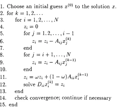
The pseudocode of block SOR is given by the following algorithm. Table 2.2 provides the number of operations per iteration in addition to the storage requirement of the method. Operations in steps 6, 9, and 11 are equivalent to 1 S A X P Y and 1 matrix vector multiplication, where each of the vector length and matrix order is n. Step 12 solves a preconditioned system and is considered as 1 Precond Solve. The two vectors that we need to store are x and 2.

If the matrix A is irreducible (which is the case in our experiments) then it is clear from (2.10) that at each iteration we are going to solve N nonhomo- geneous systems of equations with nonsingular coefficient matrices. This can be achieved by employing either direct or iterative methods. Different criteria may affect the choice of the method to be used for solving a diagonal block as there is no requirement to stick to the same method to solve all diagonal

Algorithm: Block SOR

1. Choose an initial guess to the solution x. 2. for A: = 1 ,2 .... 3. 4. 5. 6. 7. 8. 9. 10.

11

14. check convergence; continue if necessary 15. end for i = 1 ,2 , . . . , iV ^. = 0 for j = 1 .2 ,... — 1 __________________A..AD r-Lijdyj end for j = i + I , . . . , N ________ end z,· = uJZi + (1 - u)Aiixf~'·'' solve Dux^l"^ = Zi

blocks; we will come to the implementation details later in this chapter. In general, for a given coefficient matrix A, the larger the block sizes (and hence the smaller the number of blocks), the fewer the (outer) iterations needed to achieve convergence [36]. The reduction in the number of iterations is usually offset to a certain degree by an increase in the number of operations that are to be performed at each iteration. However, this is not always true as it is highly dependent on the matrix structure.

Method Inner Product SAXPY Matrix-Vector Product Precond Solve Storage Requirement

Block SOR 0 1 1 ,ya matrix+2n

Table 2.2: Summary of Operations and Storage Requirements for Block SOR at iteration k.

“ Since blocks in the partition are not necessarily o f the same size, the size of the operands in the given counts are most likely different.