Novel implantable distributively loaded flexible resonators for MRI

NOVEL IMPLANTABLE DISTRIBUTIVELY

LOADED FLEXIBLE RESONATORS FOR

MRI

A THESIS

SUBMITTED TO THE DEPARTMENT OF ELECTRICAL AND ELECTRONICS ENGINEERING

AND THE GRADUATE SCHOOL OF ENGINEERING AND SCIENCES OF BILKENT UNIVERSITY

IN PARTIAL FULLFILMENT OF THE REQUIREMENTS FOR THE DEGREE OF

MASTER OF SCIENCE

By

Sayım Gökyar

ii

I certify that I have read this thesis and that in my opinion it is fully adequate, in scope and in quality, as a thesis for the degree of Master of Science.

Assoc. Prof. Dr. Hilmi Volkan Demir (Supervisor)

I certify that I have read this thesis and that in my opinion it is fully adequate, in scope and in quality, as a thesis for the degree of Master of Science.

Prof. Dr. Ergin Atalar

I certify that I have read this thesis and that in my opinion it is fully adequate, in scope and in quality, as a thesis for the degree of Master of Science.

Prof. Dr. Üstün Aydıngöz

Approved for the Graduate School of Engineering and Sciences:

Prof. Dr. Levent Onural

iii

ABSTRACT

NOVEL IMPLANTABLE DISTRIBUTIVELY LOADED

FLEXIBLE RESONATORS FOR MRI

Sayım Gökyar

M.S. in Electrical and Electronics Engineering

Supervisor: Assoc. Prof. Dr. Hilmi Volkan Demir August 2011

Magnetic resonance imaging (MRI) is an enabling technology platform for imaging applications. In MRI, the imaging frequency falls within the radio frequency (RF) range where the tissue absorption of electromagnetic power is conveniently very low (e.g., compared to X-ray imaging), making MRI medically safe. As a result, MRI has evolved into a major imaging tool in medicine. However, in MRI, it is typically difficult to receive a magnetic resonance signal from tissue near a metallic implant, which hinders imaging of the implant device neighborhood to observe, monitor, and make assessment of the recovery and tissue compatibility. This can be accomplished by using locally resonating implants, but such implantable local resonators compatible with MRI that simultaneously feature reasonable chip size are currently not available (although there are some MRI-guided catheter applications). In this thesis, we proposed and developed a new class of implantable chip-scale local resonators that operate at radio frequencies of MRI, despite their small size, for the purposes of enhancing the signal-to-noise ratio (SNR) and thus the resolution in their vicinity. Here we addressed the scientific challenge of achieving low resonance frequency while maintaining chip-scale size suitable for potential MR-compatible implants. Using only biocompatible materials (gold, nitrides, and silicon or polyimide) within a substantially reduced footprint (miniaturized by 2 orders of magnitude), we demonstrated novel chip-scale designs based on the basic concept of split ring resonators (SRRs). Different than classical SRRs

iv

or those loaded with lumped elements (e.g., thin-film lumped loading), however, in our designs we loaded the SRR geometry in a distributive manner with a micro-fabricated dielectric thin-film layer to increase effective capacitance. For a proof-of-concept demonstration, we fabricated 20 mm × 20 mm resonators that operate at the resonance frequency of 130 MHz (compatible with 3 T MRI system) when distributively loaded with the capacitive film, which would otherwise operate around 1.2 GHz as a classical SRR of the same size if not loaded. It is worth noting that this resonance frequency of 130 MHz would normally require a classical SRR of 20 cm × 20 cm, a chip size 100-fold larger than ours. Designing and fabricating flexible thin-film resonators, we also showed that this architecture can be tuned by bending and is appropriate for non-planar surfaces, which is often the case for in vivo imaging. The phantom images indicated that, depending on the resonator configuration, these novel self-resonating structures increase SNR of the received signal by a maximum factor of 4 to 150 and over an enhancement penetration up to 10 mm into the phantom. This corresponds to a resolution enhancement in the 2D image by a factor of 2 to 12, respectively, under the same RF power. These in vitro experiments prove that it is possible to operate our local resonators at reduced frequencies via the help of distributive loading on the same chip. These findings suggest that proposed implantable resonator chips make promising candidates for self-resonating MR-compatible implants.

Key Words: Magnetic resonance imaging (MRI), thin film loading, MR-compatible implants, wearable MRI coils, inductively coupled radio frequency coils (ICRF).

v

ÖZET

MANYETİK REZONANS GÖRÜNTÜLEME İÇİN

DAĞILIMSAL YÜKLENMİŞ İMPLANT EDİLEBİLİR

ÖZGÜN ESNEK REZONATÖRLER

Sayim Gökyar

Elektrik ve Elektronik Mühendisliği Bölümü Yüksek Lisans Tez Yöneticisi: Doç. Dr. Hilmi Volkan Demir

Ağustos 2011

Manyetik rezonans görüntüleme (MRG), görüntüleme uygulamalarına imkan tanıyan bir teknoloji platformudur. MRG’nin görüntüleme frekanslarının dokuların elektromanyetik gücün emiciliğinin oldukça az olduğu radyo frekansı (RF) aralığında olması, MRG’yi diğer birçok yönteme göre (örneğin :x-ray) sağlık açısından oldukça güvenli yapmaktadır. Bunun sonucu olarak da, MRG, yaygın bir tıbbi görüntüleme yöntemi haline gelmiştir. Ancak, MRG’de, canlı içindeki metalik implantların yakınlarından genellikle görüntü sinyalinin alınamıyor olması, bu yapıların çevresinin gözlenip, izlenmesine, iyileşmenin analizine ve yapıların doku uyumluluklarına bakılmasına engel olmaktadir. Bu durum, bölgesel olarak rezone eden yapıların kullanılması ile çözülebilir, ama (her ne kadar MRG reheberli bazı girişimsel kateter uygulamaları varsa da) hem MR uyumlu hem de yeterince küçük boyutlarda bölgesel rezonatörler günümüzde mevcut değildir. Bu tezde, vücut içi implantların yakınında sinyal-gürültü oranını, dolayısıyla çözünürlüğü, artıracak küçük boyutlarına rağmen MRG frekanslarında çalışan yeni bir bölgesel rezonatör türünü önerip geliştirdik. Bununla, MR uyumlu olası implantlara uygun, yonga ebatlarında kalarak düşük rezonans frekansını elde edebilme problemini bilimsel olarak ele aldık. Yarıklı halka rezonatörlerin (YHR) temel mantığından hareketle, oldukça küçük bir baskı alanında (100 kat küçültülmüş alanda) yalnızca biyo-uyumlu malzemeler kullanarak (altın, nitrürler, ve silisyum veya polimit), yonga

vi

ebatlarında özgün tasarımları gerçekleştirdik. Klasik YHR’lerden ya da bir noktadan elemanlarla yüklenmiş (örneğin, ince film noktasal yükleme) rezonatörlerden farklı olmanın yanında, tasarımlarımızda etkin kapasitif etkiyi artırmak için YHR geometrisini dağılımsal tarzda mikro-üretimle yapılmış yalıtkan ince-filmler ile yükledik. Kavramın kanıtının gösterimi için, standart YHR olması durumunda 1.2 GHz frekansında rezone edecek, ancak dağılımsal olarak ince film ile yüklendiğinde (3T MRG sistemine uygun) 130 MHz’de rezone eden, 20 mm × 20 mm ebatlarında, yapılar ürettik. Bu ebatların, standart YHR mimarisi kullanılması durumunda, 130 MHz’de rezone edebilmesi için tasarımımızdan 100 kat daha büyük, 20 cm × 20 cm, olması gerekir. Ayrıca esnek ince-film yüklü rezonatörler tasarlayıp ve üretip, aynı zamanda bu yapının bükerek akortlanabildiğini ve düzlemsel olmayan vücut içi yüzeylerin görüntülenmesi için uygun olduğunu gösterdik. Kendi kendine rezone edebilen özgün yapılarımızın uzaydaki durumuna göre, fantom görüntüleri alınan sinyallerin şiddetlerini en fazla 4 ile 150 kata kadar ve etki derinliğini de 10 mm’ye kadar artırılabildiğini gösteriyor. Bu durum, aynı RF gücünü kullanarak, 2 boyutlu görüntülerde çözünürlüğü yaklaşık 2 ile 12 kat artırabilmeye karşılık geliyor. Bu test ortamındaki deneyler, bölgesel rezonatörlerin aynı yonga üstünde dağılımsal yüklenmeleri sayesinde çok daha düşük frekanslarda çalışmalarının mümkün olduğunu ispatlıyor. Bu bulgular, vücut içine uygulanabilir rezonatör çiplerimizin MR uyumlu kendi kendine rezone edebilen implantlar için kullanımını vaadediyor.

Anahtar Kelimeler: Manyetik resonans görüntüleme (MRG), ince film yükleme, MR uyumlu implantlar, giyilebilir MRG bobinleri, indüklenerek eşlenmiş radyo frekans (İERF).

vii

Acknowledgements

I would like to express my deepest appreciation to my supervisor Professor Hilmi Volkan Demir for his brilliant and wise comments on my research during this thesis. Not only his comments but also his endless energy and motivating personality propel me to work in a more disciplined way. He guided me through this blessed way that is long, tough and very difficult to finish without his help. I believe that the words are not enough to define his contributions to this thesis but in short, he is certainly one of the masters in his fields.

Human being crawled before he stands and walked before he runs. It is great pleasure for me to state my kind regards to Professor Ergin Atalar since he helped me to learn how to stand without crawling. He opened the doors of MRI to my life and helped us to use UMRAM (National MR Research Center) for our experiments. His invaluable discussions determined the milestones of this research work.

I would like to express my gratitude to Professor Üstün Aydıngöz for his interest and spending his valuable times to evaluate this thesis and give precious comments about it.

Although the way is long, it starts with a first step and it is important to have kind colleagues traveling with you. I would like to thank to each and every member of Devices and Sensors Group for their kind and eternal friendship. They are the indispensable part of this thesis.

I cannot forget thanking Biomedical Engineering Group members at UMRAM. They have trained me on how to use the scanner and allowed me to use their experimental workbenches.

I would like to express my special thanks to Dr. Rohat Melik for his help and synergy during my first steps in this way. His broad perspective on academic issues and sincere personality in nonacademic environment attracts me to imitate

viii

him. Together with Dr. Melik, Emre Ünal is one of my heroes in this research work. His experience on microfabrication and talent on experimental work has allowed me to make an accelerated progress in my research work.

The most exciting part of the life is the present time, which shows the continuity of the research. Actually, I think it is the most exciting instant if the scientific research is making progress. We are not searching for ordinary reasons; we are researching for the wisdom of the matter, which I think triggers the astonishment of human being.

This is the right time for me to declare my appreciation to my family. We always need reasons to do things and all of my appreciation during this thesis work has valid and valuable reasons. However, there is no reason to thank my family, because they love me without any reason. Simply, Thank YOU.

ix

Table of Contents

1. INTRODUCTION... 1

1.1HISTORY AND BACKGROUND INFORMATION OF MRI... 1

1.2MOTIVATION AND THE SCOPE OF THE THESIS... 1

2. FUNDAMENTALS OF MRI... 4

2.1BASIC CONCEPTS OF MRI... 4

2.1.1 Physics of Spin... 4

2.1.2 Frequency Characteristics of Different Nuclei ... 6

2.2FIELDS OF MRI ... 7

2.2.1 Main Magnetic Field ... 7

2.2.2 Radio Frequency Magnetic Field ... 7

2.2.3 Gradient Fields... 12

2.3HARDWARE... 13

2.3.1 Main Field Magnet ... 13

2.3.2 Gradient Field Electromagnets ... 14

2.3.3 RF Field Electromagnets ... 15

2.3.3.1 Magneto Static Field Solutions for Birdcage Coil ... 16

2.3.3.2 Equivalent Circuit Analysis of High Pass Birdcage Coil... 20

3. RESONATORS ... 23

3.1LCRESONATORS... 23

3.2RING RESONATOR ANALYSIS... 24

3.2.1 Electromagnetic Analysis ... 24

3.2.2 Resonance Frequency Analysis ... 31

3.3RECTANGULAR SRRCHARACTERISTIC... 33

4. LOADING OF RESONATORS ... 36

4.1LUMPED ELEMENT LOADING... 36

4.2THIN FILM LOADING... 39

x

4.4CIRCUIT EQUIVALENT ANALYSIS OF DISTRIBUTIVE LOADING... 50

4.4.1 Lumped model ... 51

4.5PHANTOM SIMULATIONS FOR LOSS TERM EFFECTS... 58

5. MRI OF DISTRIBUTIVELY LOADED RESONATORS ... 64

5.1MICRO-FABRICATION OF RESONATORS... 64

5.1.1 Micro-fabrication of Resonators on a Rigid Substrate... 65

5.1.2 Micro-fabrication of Resonators on a Flexible Substrate... 70

5.2RESONATORS EMPLOYED AS EXTERNAL DEVICES... 73

5.3RESONATORS EMPLOYED AS INTERNAL DEVICES... 84

5.3.1 Phantom Imaging Using Classical Resonator... 84

5.3.2 Phantom Imaging Using Novel Rigid Resonators ... 85

5.3.3 Phantom Imaging Using Novel Flexible Resonators ... 89

5.3.3.1 Planar Imaging with the Flexible Resonators ... 89

5.3.3.2 Nonplanar Imaging with the Flexible Resonators Having Different Curvatures... 94

6. CONCLUSIONS AND FUTURE WORK... 108

xi

List of Figures

Figure 2.1 Definition of spin from a) quantum mechanical and b)

classical mechanics perspectives, with c) excited spin, rotating

along B axis... 5

Figure 2.2 Excited spin with transverse magnetization and receiving

coils. ... 8

Figure 2.3 Longitudinal and transverse magnetization of fat after RF

excitation. ... 11

Figure 2.4 Transverse magnetizations of fat and muscle after

excitation. ... 11

Figure 2.5 Effect of the gradient field on emitted signal to extract

spatial point of sources. ... 13

Figure 2.6 A single excitation spin echo imaging sequence. ... 14

Figure 2.7 Coil placements of an MRI Scanner. ... 16

Figure 2.8 Example of a low pass birdcage coil... 16

Figure 2.9 B field distributions for different dimensions of square

loops... 18

Figure 2.10 Circuit equivalent of high pass birdcage coil. ... 20

Figure 3.1 Series RLC circuit. ... 23

Figure 3.2 Structure of a circular resonator a) a closed ring resonator

and b) a split ring resonator. ... 24

Figure 3.3 Field maxima of ring resonators for their first two modes:

a) for n=1, b) for n=2, c) for n=1.5, and d) for n=2. ... 26

Figure 3.4 Footprint of a) circular b) rectangular SRRs. ... 27

xii

Figure 3.6 Current distribution of the circular SRR at different

frequencies: a) at 100 MHz, b) at 500 MHz, c) at 900 MHz, d) at

1.1 GHz, e) at 1.5 GHz (on resonance), and f) 2.0 GHz. ... 29

Figure 3.7 Electric field distributions of the circular SRR at different

frequencies: a) at 100 MHz, b) at 500 MHz, c) at 900 MHz, d) at

1.1 GHz, e) at 1.5 GHz, f) at 2.0 GHz,... 30

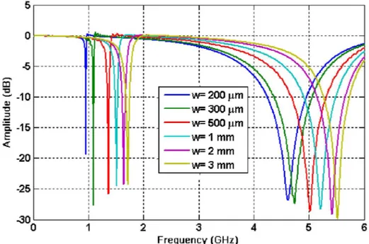
Figure 3.8 First two modes of circular SRR for different gap widths.

... 31

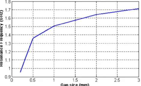
Figure 3.9 Resonance frequency as a function of the gap size for the

circular SRR. ... 32

Figure 3.10 Effective capacitance due to gap size... 33

Figure 3.11 Transmission characteristics of the circular and

rectangular SRRs. ... 34

Figure 3.12 Complete field comparisons of the circular and

rectangular resonators on resonance: E field of a) the rectangular

SRR and b) the circular SRR, and... 35

Figure 4.1 Normalized transmission of the rectangular SRR with a

footprint of 20 cm by 20 cm. ... 36

Figure 4.2 a) E-field and b) current distribution of the rectangular

SRR at resonance frequency. ... 37

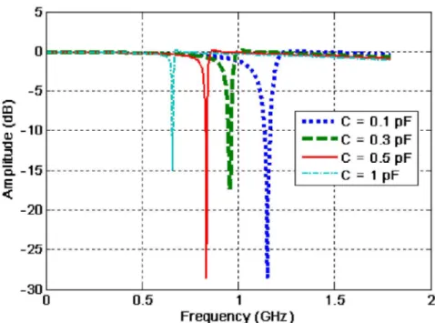
Figure 4.3 Transmission spectrum of the rectangular SRR for

different lumped capacitances... 38

Figure 4.4 Cross-section view of metal-tissue boundary... 40

Figure 4.5 Our rectangular SRR with distributively thin film loading.

... 42

xiii

Figure 4.6 Cross section view of SRR with thin film loaded region.

... 43

Figure 4.7 Normalized transmission of SRR for a dielectric film

thickness of 500 µm... 44

Figure 4.8 Amplitude of E-field distribution: a) on the lower ring and

b) on the upper overlay at the resonance frequency. ... 45

Figure 4.9 Current distribution of SRR at the resonance frequency.45

Figure 4.10 Normalized transmission of the partially loaded SRR for

various dielectric film thicknesses. ... 46

Figure 4.11 Layout of a fully distributively loaded resonator (almost

one full turn)... 47

Figure 4.12 E-field and current distribution for the novel structure

for a) E-field amplitudes on the lower ring at resonance

frequency, b) current distribution on resonance, c) E-field

distribution on the dielectric region, d) a closer look at the

current directions on resonance, e) E-field distribution on the

upper ring, and f) current distribution of the second mode. ... 49

Figure 4.13 Transmission of fully distributively loaded SRR for

various dielectric film thicknesses. ... 50

Figure 4.14 Proposed unit cell configuration for distributive loading.

... 52

Figure 4.15 Circuit equivalent of structure for n=1... 52

Figure 4.16 Circuit response for n=1. ... 53

Figure 4.17 Unit cell representation for n=2. ... 53

Figure 4.18 Circuit response for n=2. ... 54

Figure 4.19 Circuit equivalent for n=4... 54

xiv

Figure 4.21 Frequency response of the modified circuit for n=4... 55

Figure 4.22 Circuit equivalent for n=16... 56

Figure 4.23 Frequency response of the equivalent circuit for n=16. 57

Figure 4.24 Sample unit cell including the loss parameters. ... 58

Figure 4.25 Simulation layout for lossy environment. ... 59

Figure 4.26 Cross section of the simulation environment (not drawn

to on scale). ... 59

Figure 4.27 Transmission of a distributive loaded resonator inside

the phantom. ... 60

Figure 4.28 Electric field distribution of the structure for different

planes: a) 1 mm inside the phantom on the back, b) at the bottom

ring, c) in the middle of the plates, and d) at the top ring ... 62

Figure 4.29 Current distribution of the structure... 62

Figure 5.1 Layout of our chrome coated quartz mask for the lower

ring (the first metal layer). ... 66

Figure 5.2 Layout of the chrome coated quartz mask for the upper

ring (the second metal layer)... 68

Figure 5.3 Process flow for fabrication on a rigid substrate. ... 69

Figure 5.4 Process flow for fabrication on a flexible substrate... 72

Figure 5.5 MRI of the resonators with a flip angle of 5º. ... 75

Figure 5.6 Intensity level distribution along the horizontal axes of the

resonators. ... 75

Figure 5.7 MRI of the resonators with a flip angle of 10º. ... 76

Figure 5.8 Intensity level distribution along the horizontal axes of the

resonators. ... 76

xv

Figure 5.10 Intensity level distribution along the horizontal axes of

the resonators... 77

Figure 5.11 MRI of the resonators with a flip angle of 20º. ... 78

Figure 5.12 Intensity level distribution along the horizontal axes of

the resonators... 78

Figure 5.13 MRI of the resonators with a flip angle of 25º. ... 79

Figure 5.14 Intensity level distribution along the horizontal axes of

the resonators... 79

Figure 5.15 MRI of the resonators with a flip angle of 50º. ... 80

Figure 5.16 Intensity level distribution along the horizontal axes of

resonators. ... 80

Figure 5.17 Intensity amplification of the resonators for different flip

angles. ... 81

Figure 5.18 Enhancement factor due to flip angle excitation. ... 83

Figure 5.19 Enhancement limit for external imaging due to different

flip angles. ... 83

Figure 5.20 A sample image of an SRR inside the phantom. ... 84

Figure 5.21 MRI of the novel resonating structure on a rigid

substrate for a flip angle of 5°... 85

Figure 5.22 MRI of the novel resonator structure on a rigid substrate

for 10° flip angle... 86

Figure 5.23 MRI of the novel resonator structure on a rigid substrate

for 15° flip angle... 86

Figure 5.24 MRI of the novel resonator structure on a rigid substrate

for a flip angle of 20°... 87

Figure 5.25 MRI of the novel resonator structure on a rigid substrate

for a flip angle of 45°... 87

xvi

Figure 5.26 Characteristic of rigid resonator due to different flip

angles. ... 88

Figure 5.27 MRI of the novel resonator structure on a flexible

substrate for 5° flip angle (planar configuration)... 89

Figure 5.28 MRI of the novel resonator structure on a flexible

substrate for 10° flip angle (in planar configuration)... 90

Figure 5.29 MRI of the novel resonator structure on a flexible

substrate for 15° flip angle (in planar configuration)... 90

Figure 5.30 MRI of the novel resonator structure on a flexible

substrate for 20° flip angle (in planar configuration)... 91

Figure 5.31 MRI of the novel resonator structure on a flexible

substrate for 45° flip angle (in planar configuration)... 91

Figure 5.32 Comparison of the flexible and rigid resonators for

different flip angles... 92

Figure 5.33 Enhancement factor of the resonators for different flip

angles. ... 93

Figure 5.34 Enhancement limit for internal planar imaging due to

different flip angles... 93

Figure 5.35 Sketch of the flexible resonator. ... 95

Figure 5.36 Side view of the bent resonator... 95

Figure 5.37 MRI of the bent resonator for 5° flip angle (in nonplanar

configuration). ... 96

Figure 5.38 MRI of the bent resonator for 10° flip angle (in

nonplanar configuration)... 96

Figure 5.39 MRI of the bent resonator for 15° flip angle (in

xvii

Figure 5.40 MRI of the bent resonator for 20° flip angle (in

nonplanar configuration)... 97

Figure 5.41 MRI of the bent resonator for 45° flip angle (in

nonplanar configuration)... 98

Figure 5.42 Maximum intensity characteristics of the bent resonator

for different flip angles (in nonplanar configuration). ... 99

Figure 5.43 Enhancement factor of the bent structure with a

curvature of 83.3 m

(in nonplanar configuration). ... 99

Figure 5. 44 Enhancement limit of the bent structure with a curvature

of 83.3 m

(in nonplanar configuration). ... 100

Figure 5.45 Side view of the flipped and bent resonator. ... 100

Figure 5.46 MRI of the flipped and bent resonator for 1° flip angle

(in nonplanar flipped configuration). ... 101

Figure 5.47 MRI of the flipped and bent resonator for 2° flip angle

(in nonplanar flipped configuration). ... 101

Figure 5.48 MRI of the flipped and bent resonator for 3° flip angle

(in nonplanar flipped configuration). ... 102

Figure 5.49 MRI of the flipped and bent resonator for 4° flip angle

(in nonplanar flipped configuration). ... 102

Figure 5.50 MRI of the flipped and bent resonator for 5° flip angle

(in nonplanar flipped configuration). ... 103

Figure 5.51 MRI of the flipped and bent resonator for 10° flip angle

(in nonplanar flipped configuration). ... 103

Figure 5.52 MRI of the flipped and bent resonator for 15° flip angle

(in nonplanar flipped configuration). ... 104

Figure 5.53 MRI of the flipped and bent resonator for 20° flip angle

xviii

Figure 5.54 MRI of the flipped and bent resonator for 25° flip angle

(in nonplanar flipped configuration). ... 105

Figure 5.55 MRI of the flipped and bent resonator for 45° flip angle

(in nonplanar flipped configuration). ... 105

Figure 5.56 Characteristic of bent resonator due to different flip

angles. ... 106

Figure 5.57 Enhancement factor of the bent structure with a

curvature of 166.7 m

(in nonplanar configuration)... 107

Figure 5. 58 Enhancement limit of the bent structure with a curvature

of 166.7 m

(in nonplanar configuration). ... 107

Figure 6.1 A novel flexible resonator designed in the shape of a

crescent moon for MR imaging. ... 110

xix

List of Tables

Table 2.1 Gyromagnetic ratios and sensitivities of H, C, F, N and P

atoms. ... 6

Table 2.2 Relaxation time values for some of the tissues at 1.5 and

3.0 T. ... 10

Table 4.1 Comparisons of computed resonance frequencies L is

calculated as 60 nH [14]. ... 39

Table 4.2 Resonance frequencies changing due to the different

1

Chapter 1

INTRODUCTION

1.1 History and Background Information of MRI

The short story of magnetic resonance imaging (MRI) started early 1970s, with the seminal work of Paul Lauterbur, which was later awarded a Nobel Prize in 2003. This late payback was due to the great contribution of Lauterbur to the nuclear magnetic resonance (NMR) instead of MRI. Relatively long story of NMR started at the beginning of this century. Upon discovery of spins, the relationship between the magnetic field and the resonance frequency of these spins was first explained by the Irish physician, Joseph Larmor. (His governing equation will be given and explained in the second chapter of this thesis.)

However, the real inventors of NMR were different; it took almost 50 years to propose the idea that this property can be used to identify different materials. In 1946, two genius researchers, Felix Bloch from Stanford University [1] and Edward Mills Purcell from Harvard University [2], independently achieved the first NMR identification of materials for liquids and solids. They shared the Nobel Prize in physics in 1952 [3]. This is the starting point of NMR for chemical identification and new concepts have been investigated to understand material behavior under magnetic field since then.

Humanity would have to wait until 1973 to see the first MRI of medical tissues

[8]. The name of the hero, who has realized this dream, was Paul Lauterbur. His inventions of magic fields, called gradient fields, are still one of the greatest research topics of MRI community [4].

1.2 Motivation and the Scope of the Thesis

This thesis aims to design and demonstrate a new class of self-resonating chip-scale structures that operate at the predetermined frequency of MRI and the characterization of these resonators both for in-phantom and ex-phantom cases.

2

Analysis under both conditions is necessary to foresee potential applications of these novel structures. The external case can be a starting point for wearable antennas while the internal case can be a milestone for self-resonating MRI compatible implants, where the latter has never been investigated in the literature to date.

Obtaining MRIs with high resolution without increasing the acquisition time and decreasing its SNR is a challenging task in most of the cases. For the treatment of epilepsy diseases, it is a common method to use subdural electrodes to image defected parts of the brain, where the positioning of the electrodes has crucial importance for the surgery [5]. The correct positioning of subdural electrodes, which cannot be seen in MRI without MR visible coatings, determines the success of the surgery.

Classical solution to this problem requires two steps to estimate the position of the subdural electrodes correctly. The first step requires the MRI, which shows the details of the brain clearly, of the environment for the mapping of soft tissues. The second step includes the computerized tomography (CT) of the metallic electrodes with the skull to map their positions on the brain. By using both of the images, approximate places of the electrodes obtained and the surgery area is determined due to these observations.

To determine the positions of subdural electrodes using only MRI, we propose the distributively loaded thin film resonating structures that can be implanted to the body with the subdural electrodes during the pre-surgical evaluation period. This method allows one to evaluate the positions of the electrodes without using CT images and with a great correctness. To achieve this, we designed, fabricated and characterized a chip-scale resonating structure, which can be further used for implantable devices for other surgical procedures.

This thesis starts with a short introduction to MRI presenting its fundamental principles and imaging methods (Chapter 2). This brief introduction prepares readers to be familiar with the relationship between the material types and their MRIs. It continues with the magnetic fields of MRI and their coils for imaging.

3

A relatively detailed analysis of RF coils stresses the importance of resonance and reviews the main properties of an antenna for MRI.

In the following chapter, Chapter 3, the classical resonance characteristics of conventional resonators are investigated and their complete electromagnetic analysis with simulations is provided. The circuit equivalent model and the current distributions together with the electric field confinement properties of split ring resonators (SRRs) are also presented here.

Chapter 4 introduces the new method of thin film distributive loading for local resonators to achieve lower resonance frequencies. It further continues with the detailed electromagnetic and circuit equivalent analysis of these self-resonating structures, called distributively loaded resonators. A unit cell approach and cascaded system models are given for and the characteristic analysis based on the given circuit models are performed using circuit theory simulation tools. Finally, Chapter 5 deals with the explanation of microfabrication processes for different designs and their characterization using MRI. Tuning of these structures to 123 MHz for 2.89 T MRI system at UMRAM [6] and their mechanical properties are discussed and then the detailed analysis of these resonators explained. Experimental work is presented in this chapter for resonators serving as external and internal devices. Phantom images for different flip angles and different device configurations are analyzed and the most striking images are included. The thesis is completed with concluding remarks and outlook in Chapter 6.

4

Chapter 2

FUNDAMENTALS of MRI

Before the seminal work of Lauterbur in 1973, NMR was a powerful method to understand the content of gaseous mixtures that can only achieve material identification. A clear understanding of NMR was necessary to figure out the basic principles of MRI that is described as the behavior of a nucleus under a certain magnetic field. The details of NMR can be accurately explained by quantum mechanics. Here, we will explain NMR using the principles of classical mechanical model with the contribution of quantum mechanics.

2.1 Basic Concepts of MRI

2.1.1 Physics of Spin

Quantum mechanics defines a fundamental property of nucleus called spin, which is due to the rotation of protons along their axis. From a classical mechanics perspective, this rotating positively charged small object with a mass exhibits angular momentum in the direction of rotation axis, and its net charge movement will result in current, which in turn, produces a magnetic field. Therefore, if we apply an external magnetic field to the proton, its angular momentum will be aligned along the direction of the applied field. Quantum mechanics explains the magnetic resonance by using the notion of energy quantization. It states that, when an external magnetic field is applied to a system, the energy levels of this system will be divided into two distinct energy levels. These defined levels are -1/2 (the highest energy state, against magnetic

field direction) and +1/2 (the lowest energy state, through magnetic field

direction). The energy difference between these two states is given by Equation (2.1).

5 ω π 2 h E = ∆ (2.1)

where h is the Planck’s constant and ω is the angular frequency (in rad/s) corresponding to the spinning frequency of the proton. For a nucleus with an even number of spins, each of every two protons has opposite energy level that cancels each other and results in zero net magnetic moment (mr_s). Such nuclei do not interact with the external magnetic field; thus, we are not interested in these atoms. On the other hand, atoms with odd number of protons exhibit good NMR characteristics and it is impossible to obtain zero net magnetic moment for any configuration of their spins. To visualize these, let us have a look at Figure 2.1

Figure 2.1 Definition of spin from a) quantum mechanical and b) classical mechanics perspectives, with c) excited spin, rotating along B axis.

Here, Br represents the magnetic field vector and Mr is the total magnetization vector of nuclei with amplitude of M0. If it is a single 1H, then it is the

magnetization of a single proton and can be represented byms

r

. Total net magnetization (M0) is the macroscopic parameter, as opposed to the

6

2.1.2 Frequency Characteristics of Different Nuclei

At the beginning of the 20th century, Joseph Larmor (1857), an Irish physician, proposed a formula that defines the relationship between the external magnetic field and the angular frequency of the spins as given in Equation (2.2).

B γ

ω = (2.2) Here, B is the magnetic field intensity (tesla) and ω is the angular frequency (rad/s) of the nuclei. This expression emphasizes the linear relationship between the rotational frequency and the external magnetic field with a characteristic coefficient known as gyromagnetic ratio (γ). The gyromagnetic ratios and sensitivities of some atoms are given in Table 2.1 [7]. Sensitivity of an atom is defined as the MRI signal emission ratio of an atom after excitation.

Atom 1H 13C 19F 23N 31P

γ/2π (MHz/T) 42.575 10.705 40.054 11.262 17.235

Relative Sensitivity 1.000 0.016 0.830 0.093 0.066

Table 2.1 Gyromagnetic ratios and sensitivities of H, C, F, N and P atoms.

After these explanations, we now explain medical imaging frequencies. Hydrogen atom (1H), which is abundant in all organic tissues, has the key role in determining the operating MR frequency. Commercially available MRI scanners with B of 1.5 T and 3 T are commonly used at the corresponding hydrogen resonance frequencies of 63.8 and 127.7 MHz, respectively. Depending on typical B values adapted in the MRI, the imaging frequency falls within the radio frequency (RF) range where the tissue absorption of electromagnetic (EM) power is conveniently very low (e.g., compared to X-ray imaging).

7

2.2 Fields of MRI

2.2.1 Main Magnetic Field

As we mentioned in the previous section, the direction of magnetic moment of the spins will be parallel to the direction of the magnetic field, thus having non-zero net magnetization. Since the net macroscopic magnetic moment (M0) is the summation of microscopic magnetic moments, which are randomly oriented in the absence of external magnetic field with zero net magnetization, it will be an obligation to apply a unidirectional, time independent (DC), homogeneous magnetic field. Nuclei under such a homogeneous field will exhibit uniform magnetization vector pointed in the magnetic field (B) direction called the longitudinal direction, which is commonly taken as the z-direction. It should be noted that DC magnetic field, which is used to obtain a total net nonzero magnetization, does not excite the spins to transmit magnetic energy to the environment. To sum up, we only have magnetized spins resonating at a Larmor frequency inside the given DC field (Figure 1.b), but not rotating along any axis or emitting any signal to capture for imaging.

As mentioned earlier, commercially available MRI scanners for medical imaging with magnetic flux densities (B) from 0.1T to 3 T are commonly used at the corresponding hydrogen resonance frequencies from 4.26 MHz to 127.7 MHz, respectively. There are also high field NMR scanners with the B field strength of up to 25 T for material identification.

2.2.2 Radio Frequency Magnetic Field

As we see in Figure 1.b, DC magnetic field causes nucleus to spin along its direction. The excitation of spins, in other words their rotation along longitudinal direction, should be achieved to allow them to transmit their magnetization as illustrated in Figure 1.c. Since nuclei are spinning at the given Larmor frequency, the excitation signal should also be have the same frequency to rotate spins coherently. Now we have the combination of two motions,

8

rotation along the longitudinal axis and spinning along this rotating axis at the same frequency. Flip angle, the angle between the magnetization vector (M0)

and the longitudinal direction, will determine the amount of signal that will be transmitted to the receiver antennas, located at the transverse plane, as sketched in Figure 2.2.

Figure 2.2 Excited spin with transverse magnetization and receiving coils.

In three-dimensional space, the excited magnetization vector will have components not only in z-direction, but also on x-y plane. If the value of flip angle is 90º then the magnetization vector will completely lie on the transverse plane. The net magnetization can now be implemented by two components, Mz

and Mxy. The rotating nature of magnetization, not the spinning, will result in net

current, thus an electromagnetic radiation emitted from the nuclei at the Larmor frequency can be detected by the receiver antennas. In MRI systems, the excitation typically takes place in the first few milliseconds and the rest of the duration before the next excitation is reserved for signal reception, which can last for several seconds.

After the excitation of nuclei, rotation of spins along longitudinal axis will continue only for a certain amount of time. Since there is a time invariant magnetic field in the z-direction, the net magnetization will tend to be aligned

9

along the z-direction, which is known as recession. We can infer that the transverse magnetization will decrease as the time elapses, resulting in decreased in signal reception over time. On the other hand, longitudinal magnetization will increase to its initial value, M0. The nature of recession is

identified by two specific coefficients, T1 and T2, called longitudinal and transverse relaxation constants, respectively. At this point, we should have a short look at the Bloch equation.

Assume Mr(t) is defined with its scalar components Mx, My and Mz in the

directions of x, y and z, respectively. For the sake of simplicity, we will be using i, j and k for the directions of x, y and z; then, the popular Bloch equation can be written as in Equation (2.3): 1 ˆ ) ( 2 ˆ ˆ 0 T k M M T j M i M B M dt M d x y _z − − + − × = r r r γ (2. 3)

When we analyze this differential equation separately, we can express the longitudinal relaxation as in Equation (2.4).

1 0 T M M dt dM_{z z} − − = (2. 4)

This has the solution in the form of exponential function as follows:

) 1 ( ) ( 0 / 1 T t z t M e M = − − (2. 5) The transverse relaxation equation becomes as in Equation (2.6).

2 T Mxy dt dMxy − = (2. 6)

with a solution given as:

2 / 0 ) ( t T xy t M e M = − (2. 7) where Mxy is the vector summation of Mx and My and given in Equation (2.8)

y x xy ıM jM

10

Equation 2.8 states that the vectorial summation of transverse magnetization decays exponentially. From previous explanations, we already know that it is also a rotating field due to the left hand rule, which means that another time dependent parameter should be added. Mathematical expressions for a complete solution are given as follows [7].

t f i T t xy

M

e

e

M

=

1.5 T 3.0 T Tissue T2 (ms) T1 (ms) T2 (ms) T1 (ms) Gray matter 100 900 100 1820 White matter 92 780 70 1084 Muscle 47 870 45 1480 Fat 85 260 83 490 Liver 43 500 42 812

Table 2.2 Relaxation time values for some of the tissues at 1.5 and 3.0 T.

By Equations 2.5 and 2.7, we can calculate the longitudinal and transverse components of magnetization for fat with unity initial magnetization (M0) at 1.5 T as shown in Figure 2.3.

11

Figure 2.3 Longitudinal and transverse magnetization of fat after RF excitation. As clearly seen from Figure 2.3, the transverse magnetization decays very fast, which means its imaging signal should be recorded at the beginning of the excitation. To understand the importance of relaxation parameters, let us have a look at the Figure 2.4 for contrast between different tissues.

12

Figure 2.4 states that, under the same imaging conditions, the decay of transverse magnetization of fat is slower than the decay of transverse magnetization of muscle. We can roughly claim that, with the same amount of nuclei, fat will emit more signal than muscle at any instant of imaging due to its slowly decaying transverse magnetization thus can be seen brighter than muscle in the received image. However, we have to remember that it is too early to speak about the contrast between tissues since the opposite can also happen due to the other imaging parameters.

2.2.3 Gradient Fields

It is clear that the material identification can be achieved by using static and RF magnetic fields due to the characteristic coefficients of materials such as: γ, T1 and T2,. However, mapping the spatial distribution of materials, locating the signal sources in three-dimensional spaces, is not possible with only these two fields. Since the signal coming from all of 1H nuclei in any substance has the same frequency, the receiver coils will detect a signal that has a single frequency and amplitude. By using amplitude data, it will be possible to obtain, which substances are being imaged, but their physical coordinates cannot be determined.

Paul Christian Lauterbur, an American chemist, proposed that introducing gradient fields into the imaged medium would make it possible to map the sources of emitted signals. It was the beginning of 70’s when he first obtained the first medical MRI images [9]. Later on his awesome work was awarded with a Nobel Prize in Physiology or Medicine in 2003, shared with Peter Mansfield [10].

Introducing gradient fields to the imaging medium will change the spinning frequency of nuclei that results in a bandwidth of absorbed/emitted signal. The detected signal now has different frequencies associated with their physical coordinates and amplitudes related to their material types.

13

Figure 2.5 Effect of the gradient field on emitted signal to extract spatial point of sources. Figure 2.5a, shows an exponentially decaying signal with a single frequency, whereas the Figure 2.5b shows another decaying signal, which seems to be a modulated by another frequency. Due to the bandwidth of the emitted fields from nuclei, Fourier transform of this modulated signal will be in rectangular, with each of its frequencies corresponding to a spatial point in space. The detailed mathematical expressions related to the gradient fields and RF excitation can be found in Ref 7.

2.3 Hardware

2.3.1 Main Field Magnet

Since the main magnetic field determines the resonance frequency, this magnet can be renamed as the identity of the system. Although permanent magnets can be used as the open coils for the patients with claustrophobia, this is mostly an electromagnet constructed as a solenoid to produce uniform magnetic field

14

inside it. To eliminate non-uniformities due to other equipment, shimming coils are also included inside [11].

2.3.2 Gradient Field Electromagnets

As we mentioned in the previous section, gradient fields are responsible for image construction. They are effective at slice selection, determination of phase and frequency distribution. Their dimensions are comparable with the scanner’s, and thus they have very high inductance that can create high voltages in the case of instant current deviations. Since they are working only at the specific instances of imaging, they should easily be turned on and turned off. For a typical imaging sequence as shown in Figure 2.6, gradient fields are generally activated in the range of T2 duration, which is too short to switch on and off such a high inductance. There are sophisticated circuitry and physical designs such as including shielding of coils that overcome such problems [12].

15

In Figure 2.6, slice selection should be performed simultaneously with the RF excitation. Direction of the applied gradient field determines the orientation of the imaging plane and the rest of two gradient fields will be responsible from frequency and phase distributions. Free induction decay (FID) is the NMR signal that is emitted from the imaged object to be used for imaging. TE is the instant at which the signal emitted from the nuclei becomes the maximum and the hardware of the scanner is adjusted to receive and store the data.

2.3.3 RF Field Electromagnets

This is the most interesting topic about the electromagnetic of MRI. This topic is much more complicated than we are interested; we will only introduce the necessary information and focus on the current distribution of electrically resonating structures. Since nuclei are spinning at Larmor frequency along magnetic field, to achieve the resonance condition, it should be excited at the same frequency to rotate along the same axis. We already mentioned that the angular momentum, in other words the magnetization vector, of the spin would be directed toward the magnetic field direction. If we apply a transverse magnetic field to the system, the resultant field will make an angle, called the flip angle, with the longitudinal direction. If the amplitude of transverse magnetic field is rotating in x-y plane, then the tip of the magnetization vector will also follow that resultant field at the frequency of rotation. If these rotational and spinning frequencies are the same, then the magnetic resonance condition will occur. To achieve this condition, several coils will be placed perpendicular to the radial direction of the imaging space and will be turned on and off sequentially. There are fantastic RF designs, for example, called birdcage coils that have uniform field distribution in the region of interest. Birdcage coils also combine the coils by proper electrical connection, leading to a single structure that resonates at the necessary frequency band. The principle MRI magnet configuration can be seen in Figure 2.7 and a low pass birdcage coil is shown in Figure 2.8.

16

Figure 2.7 Coil placements of an MRI Scanner.

Figure 2.8 Example of a low pass birdcage coil.

2.3.3.1 Magneto Static Field Solutions for Birdcage Coil

Before going into details of birdcage coil, we must review the effect of current distribution on magnetic field pattern. Time independent electric current produces a steady magnetic field and the differential equations regarding this is given in Equation (2.10) and Equation (2.11):

0 = Β • ∇r r (2.10) Jr r r 0 µ = Β × ∇ (2.11)

17

where, J is the electrical current density (A/m) and μ0 is the magnetic

permeability of free space (4 π ×10−7 H·m−1). By applying the vector identity in Equation (2.12) to the Equation (2.11) we can derive the Equation (2.13) also called continuity equation.

0 ) (∇×Α = • ∇r r r (2.12) 0 = • ∇r Jr (2.13) To solve the Equation (2.10), called Gauss’ magnetic law, we introduce a fictitious field quantity called magnetic vector potential Ar as given in Equation (2.14):

A

Br=∇r× r (2.14) When we substitute Equation (2.14) into Equation (2.11), we can get Equation (2.15): J Ar r r r 0 µ = × ∇ × ∇ (2.15) This can be simplified to Equation (2.16):

J A Ar r r r r 0 2 ₌µ ∇ − • ∇ ∇ (2.16) According to the vector theorems, both divergence and curl of a vector should be defined for a solution with an additive constant. Therefore, we need to define the divergence of the vector magnetic field. To simplify the previous equations, we defined divergence as in Equation (2.17):

0

= •

∇r Ar (2.17) Thus the Equation (2.16) can be rewritten as in Equation (2.18):

J

Ar ₀ r

2 ₌₋µ

∇ (2.18) This is the well-known Poisson’s vector equation and has the solution in the form of Equation (2.19).

18 ' ) ' ( 4 ) ( ' 0 ν π µ d R r J r A V

∫∫∫

where the parameter R is given in Equation (2.20):

|' |r r

R= v−r (2.20) Substituting Equation (2.19) into Equation (2.14) yields the necessary formula for the magnetic calculations. For a line current with constant amplitude I0, the

magnetic field is given as in Equation (2.21):

∫

Equation 2.21 states that calculation of magnetic field from induced current is straightforward given the current. As an example, let us have a look at the Figure 2.9, which gives the magnetic field pattern of a square loop along its central direction with a side length of w and a current level of 1 A. This trend is also similar to the circular loop with a small intensity enhancement at the center [12].

19

By using the Biot-Savart’s formula, given in Equation 2.18, we can derive the transmission pattern of any coil with a given current distribution. Reception and transmission pattern will be the same due to the reciprocity.

At this point, we have to derive another relation to understand the effect of cylindrical and spherical surface currents on source free regions. Maxwell’s equations can be rewritten as in Equations (2.22) and (2.23):

0 = Β • ∇r r (2.22) 0 = Β × ∇r r (2.23) We now define a fictitious field ψ called the scalar magnetic potential with the property given in Equation (2.24):

Ψ ∇ − = r r B (2.24) By substituting into Equation (2.22), we obtain Equation (2.25):

(

)

ρ

φ

ρ

φ

φ

∑

Here Am and Bm are the constants computed using the boundary and source

conditions. By applying (2.24), Br can be rewritten as in Equation (2.27):

∑

∑

+

+

+

−

=

m

B

m

A

m

m

B

m

A

m

B

)

cos

sin

(

ˆ

)

sin

cos

(

ˆ

)

,

(

φ

φ

ρ

φ

φ

φ

ρ

ρ

φ

ρ

r

As an important example, surface current distribution given in Equation (2.28) φ sin ˆJ₀ z Js = r (2.28)

20

has a Br field distribution given in Equation (2.29) [12]. 2 ˆ ) , ( _x 0J0 Br ρ φ = µ (2.29) The field distribution inside a cylinder with a sinusoidal surface current distribution on z direction is a constant. This is the starting point of a birdcage design.

2.3.3.2 Equivalent Circuit Analysis of High Pass Birdcage Coil

High pass birdcage coil, given in Figure 2.8, is a circular loop, with longitudinal and circular conducting lines, called legs and rungs, respectively. Rungs also include lumped capacitors to control the current distribution and let the circuit resonate at the predetermined frequency. If capacitors were placed only at the legs, then the coil will be named low pass birdcage coil. If both legs and rungs have lumped capacitors, then the coil will be named hybrid birdcage coil. In either type of the coil, the analysis will be the same in terms of circuit equivalent parameters. Here we will only concentrate on the high pass birdcage coil. The circuit equivalent of the coil is given in Figure 2.10.

Figure 2.10 Circuit equivalent of high pass birdcage coil.

To simplify the circuit equations, let’s choose all the capacitor values (C), inductor values (L), and self inductor terms (M) equal to each other. For the sake

21

of simplicity, ignore the mutual inductances, which affect the overall resonance solution less than 10%.

By using Kirchhoff’s voltage law for the loop consisting of j and j+1th legs and jth rungs, we can write Equation (2.30).

N j I C i LI i I I M i I I M i ( _j − _{j 1})− ( _j− _{j 1})−2 _j + 2 _j =0, =1,2,..., − ω − ω + ω _ω (2.30) Here Ij is the mesh current for the jth loop. Further simplifications lead to

Equation (2.31). N j I M L C I I M( _j+1+ _j−1)+2( 1₂ − − ) _j =0, =1,2,..., ω (2.31)

Since the birdcage coils are cylindrically symmetric with N legs, the solutions of Ij must satisfy Equation (2.32)

j N j I

I ₊ = (2.32)

which leads to N linearly independent solutions, modes, as in Equation (2.33).

      − = = = 1 2 ,... 3 , 2 , 1 2 sin 2 ,..., 2 , 1 , 0 2 cos ) ( N m N mj N m N mj I_{j m} M π π (2.33)

(Ij)m denotes the current of Ij in the mth solution. To find the total current on the

jth leg, we need to subtract Ij-1 from Ij thus results in Equation (2.31).

        − = − = − − = − − 1 2 ,..., 2 , 1 ) 2 1 ( 2 cos sin 2 2 ,..., 1 , 0 ) 2 1 ( 2 sin sin 2 ) ( ) ( ₁ N m N j m N m N m N j m N m I I_{j m j m} π π π π (2.34)

It is clear that the solution for m=1 is very similar to sin(φ) or cos(φ), which produces a very uniform transverse magnetic field distribution inside the coil.

22

From the principles of MRI and derived equations, we concluded that the current distribution and amplitude determines the magnetic field pattern of a coil. Uniformity of RF field pattern and high field intensity are required for better imaging. All of the previous equations were dependent on current, which should be optimized to have better patterns. Since we are using LC type circuits to control current distribution on an RF coil, it is crucial to maximize current amplitude at the same time. Maximization of current amplitude simply depends on minimization of impedance of the circuit. From basic circuit theory, we know that the total impedance of an LC circuit at the resonance frequency is zero. This opens a new perspective to us to design new resonant structures with a desired current distribution. After a brief description of ring resonators in the following chapter, we will investigate the characteristics of a new design in the upcoming chapters.

23

Chapter 3

RESONATORS

3.1 LC Resonators

In RLC circuits, the frequency where the inductive and capacitive characteristics neutralize each other called the resonance. At the resonance, large oscillations occur. To further study RLC circuits, lets’ have a look at the following circuit and analysis.

Figure 3.1 Series RLC circuit.

Zin is the input impedance seen by the left port of the circuit and formulated by

Equation (3.1). C j L j R Z_in ω ω + 1 + = (3.1) Here ω is the angular frequency, R is the resistance, L is the inductance and C is the capacitance of the system, respectively. One can easily conclude that the resonance frequency can be written as in Equation (3.2).

LC

r

1

=

ω (3.2)

The input impedance of the circuit at the resonance frequency is computed by substituting Equation (3.2) into Equation (3.1) as in Equation (3.3)

R

24

The quality factor of a circuit, is the ratio of stored energy to the dissipated energy per cycle, is given by Equation (3.4).

C L R R L cycle one in disspiated Energy cycle one in stored Energy f Q=2π =ω = 1 (3.4)

Since the impedance of a system is the minimum at the resonance frequency, the current running in the system becomes the maximum on resonance, which is the desired case for RF coil design in MRI. Next section will help us to visualize current distribution on a ring resonator for different frequencies and their analytical solutions for field patterns.

3.2 Ring Resonator Analysis

3.2.1 Electromagnetic Analysis

Ring resonators are an example of transmission lines designed as closed loops in a certain shape such as circular and rectangular (or any other geometrical structure). The most basic one is of course a circular ring resonator, given in Figure 3.2.

Figure 3.2 Structure of a circular resonator a) a closed ring resonator and b) a split ring resonator.

25

These resonators can be fabricated on a substrate with a ground plane coated on the backside, and excited by using micro-strip transmission lines from desired points. For double micro-strip feed lines, the wavelength of a guided wave in a micro-strip ring resonator is given by Equation (3.5)

n r

g

π

λ = 2 (3.5)

Where r is the diameter of the ring and n is an integer, which represents the mode number. For a single feed line, this is given by Equation (3.6).

n r

g

π

λ = 4 (3.6) So, a single feed line structure supports longer wavelengths, (or equivalently smaller frequencies). Details of feeding and coupled line analysis can also be found at Ref.13.

Solving Maxwell’s equations in circular coordinates for this resonator system with TM excitation

(

)

{

}

φ

{

}

{

}

with the boundary condition of

0

=

φ

H at r=ri and r0 (3.10)

where A and B are constants and k is the wave number, ω is the angular frequency, Jn is the Bessel function of the first kind with an order of n and Nn is

the second kind Bessel function with an order of n. Jn' and Nn' are the derivatives

of their original functions. Applying boundary conditions leads to an eigenvalue equation, which includes the solutions of resonance frequencies [13].

26

As seen in this example, analytical solutions to the modes of a resonator, even in a single and fixed excitation point, are laborious and make the design of practical applications cumbersome. Instead, we can check the field distribution of ring resonators for different modes calculated by the help of computational tools. For example for a double port-excited system, the field maximums are depicted as in Figure 3.3 for the first two modes [13]:

Figure 3.3 Field maxima of ring resonators for their first two modes: a) for n=1, b) for n=2, c) for n=1.5, and d) for n=2.

As seen from the Figure 3.3, modes with integer multiples have field maximum near the port coupling gaps. This was expected and theoretically shown in literature [13].

Since split ring resonators (SRR) offer more flexible resonant characteristics than closed ring resonators, we will concentrate on the field and current distribution of SRRs from now on. To find the resonance frequency of a SRR,

27

we performed EM simulations by using a finite integral method (FIM) solver of CST Microwave Studio®. For these simulations, a circular ring was placed on a 380 µm thick silicon wafer that has the dimensions of 30 mm by 30 mm and the ring was set to have a diameter of 20 mm with 1 mm wide gold lines and has the thickness of 20 µm. the gap size set to 1 mm to keep aspect ratio reasonable. The structure of this SRR is shown in Figure 3.4(a).

Figure 3.4 Footprint of a) circular b) rectangular SRRs.

28

Figure 3.5 Transmission of a circular SRR.

The first two modes can be seen in Figure 3.5. Since we will be interested in lower order modes, we investigate the current distribution of the structure for several frequencies lower than the first mode as in Figure 3.6.

29

Figure 3.6 Current distribution of the circular SRR at different frequencies: a) at 100 MHz, b) at 500 MHz, c) at 900 MHz, d) at 1.1 GHz, e) at 1.5 GHz (on resonance), and f) 2.0

GHz.

It is evident that the current amplitude is at the peak level when the frequency is at the resonance value of 1.5 GHz. Only the current amplitude is not enough to justify our claims that the resonance is the best case for a coil to improve its MRI performance. We should check the E-field distribution of the resonator.

30

This will give idea us an idea about where the electromagnetic field is confined and at what frequency is the volume of the field amplification is maximized. Let us have a look at the E field patterns at different frequencies in Figure 3.7.

Figure 3.7 Electric field distributions of the circular SRR at different frequencies: a) at 100 MHz, b) at 500 MHz, c) at 900 MHz, d) at 1.1 GHz, e) at 1.5 GHz, f) at 2.0 GHz, It is clear that the E-field intensity is higher for 1.5 GHz and the field is confined at the resonator gap location, which can be controlled, and specific absorption

31

ratio (SAR) of the body can be minimized by isolating this part from the living tissue.

After this brief analysis of a circular ring resonator, it is time to understand the relationship between its resonance frequency and physical dimensions. The most effective parameter, as can be seen from the previous discussion, is the gap size. The capacitive region confines the E-field and thus controls the resonance frequency. Next section discusses this issue in detail.

3.2.2 Resonance Frequency Analysis

For a plane wave excitation, which means no coupling to the source or any other measurement equipment, SRRs have the equivalent circuit given in Figure 3.1. For an SRR, inductance is due to its conducting lines and geometry, whereas capacitance is due to its gap and self-capacitance of the metallic lines. To analyze the effect of gap capacitance on the resonance frequency, we performed the electromagnetic simulations. Transmission of the SRR structure is analyzed for each gap size and their magnitudes (in dB scale) are depicted in Figure 3.8.

32

As seen from Figure 3.8, decreasing the gap size increases the gap capacitance, to decreases the resonance frequency. To understand the model better, let us analyze the first mode resonance frequency and the corresponding effective capacitance of the gap.

Figure 3.9 Resonance frequency as a function of the gap size for the circular SRR. Figure 3.9 is derived from the Figure 3.8 that shows the relationship between the gap size and the resonance frequency. Inductance, which is only dependent on the size of conducting lines, does not change significantly with such gap size change, and thus, allow us to conclude that the frequency change is due to the variations in the gap capacitance. The inductance of the circular ring is calculated to be 60 nH [14]. Given resonance frequency, we can extract the effective capacitance for each frequency as in Figure 3.10.