Robust adaptive algorithms for underwater acoustic channel estimation and their performance analysis

ROBUST ADAPTIVE ALGORITHMS FOR

UNDERWATER ACOUSTIC CHANNEL

ESTIMATION AND THEIR PERFORMANCE

ANALYSIS

a thesis submitted to

the graduate school of engineering and science

of bilkent university

in partial fulfillment of the requirements for

the degree of

master of science

in

electrical and electronics engineering

By

Iman Marivani

September 2017

Robust Adaptive Algorithms for Underwater Acoustic Channel Esti-mation and Their Performance Analysis

By Iman Marivani September 2017

We certify that we have read this thesis and that in our opinion it is fully adequate, in scope and in quality, as a thesis for the degree of Master of Science.

S¨uleyman Serdar Kozat(Advisor)

Tolga Mete Duman

C¸ a˘gatay Candan

Approved for the Graduate School of Engineering and Science:

Ezhan Kara¸san

ABSTRACT

ROBUST ADAPTIVE ALGORITHMS FOR

UNDERWATER ACOUSTIC CHANNEL ESTIMATION

AND THEIR PERFORMANCE ANALYSIS

Iman Marivani

M.Sc. in Electrical and Electronics Engineering Advisor: S¨uleyman Serdar Kozat

September 2017

We introduce a novel family of adaptive robust channel estimators for highly chal-lenging underwater acoustic (UWA) channels. Since the underwater environment is highly non-stationary and subjected to impulsive noise, we use adaptive filtering techniques based on minimization of a logarithmic cost function, which results in a better trade-off between the convergence rate and the steady state performance of the algorithm. To improve the convergence performance of the conventional first and second order linear estimation methods while mitigating the stability issues related to impulsive noise, we intrinsically combine different norms of the error in the cost function using a logarithmic term. Hence, we achieve a com-parable convergence rate to the faster algorithms, while significantly enhancing the stability against impulsive noise in such an adverse communication medium. Furthermore, we provide a thorough analysis for the tracking and steady-state performances of our proposed methods in the presence of impulsive noise. In our analysis, we not only consider the impulsive noise, but also take into account the frequency and phase offsets commonly experienced in real life experiments. We demonstrate the performance of our algorithms through highly realistic experi-ments performed on accurately simulated underwater acoustic channels.

Keywords: Underwater communications, robust channel estimation, logarithmic cost function, impulsive noise, performance analysis, carrier offsets.

¨

OZET

SUALT˙I AKUSTIK KANAL KESTIRIMINDE SA ˘

GLAM

ADAPTIF ALGORITMALAR VE PERFORMANS

ANALIZI

Iman Marivani

Elektrik ve Elektronik M¨uhendisli˘gi, y¨uksek lisans Tez Danı¸smanı: S¨uleyman Serdar Kozat

Eyl¨ul 2017

Son derece zorlu sualtı akustik kanalları i¸cin yeni bir adaptif sa˘glam kanal tahmincileri ailesini sunuyoruz. Sualtı ortamı olduk¸ca hareketli oldu˘gundan ve d¨urt¨usel g¨ur¨ult¨uye maruz kaldı˘gından, logaritmik bir maliyet fonksiyonunun k¨u¸c¨ult¨ulmesine dayanan adaptif tekrarlamalı teknikler kullanırız ki, yakınsama oranı ile algoritmanın kararlı durum performansı arasında daha iyi bir denge olu¸sur. D¨urt¨usel g¨ur¨ult¨uye ili¸skin istikrar sorunlarını hafifletirken geleneksel birinci ve ikinci dereceden do˘grusal tahmin y¨ontemlerinin yakınsama perfor-mansını arttırmak i¸cin, logaritmik bir terim kullanarak maliyet fonksiyonundaki hatanın farklı normlarını ¨oz¨unde birle¸stirdik. Bu nedenle, olumsuz bir ileti¸sim ortamında d¨urt¨usel g¨ur¨ult¨uye kar¸sı istikrarı olumlu bir ¸sekilde artırırken, daha hızlı algoritmalara kıyaslanabilir yakınsama oranı elde ediyoruz. Ayrıca, d¨urt¨usel g¨ur¨ult¨u varlı˘gında ¨onerilen y¨ontemlerin izlenmesi ve sabit durum performansları i¸cin kapsamlı bir analiz yapıyoruz. Analizlerimizde, sadece d¨urt¨usel g¨ur¨ult¨uy¨u de¨uil, aynı zamanda ger¸cek ya¸sam deneylerinde sık¸ca kar¸sılaılan frekans ve faz uzantılarını da dikkate alıyoruz. Do˘gru ¸sekilde sim¨ule edilmi¸s sualtı akustik kanal-ları ¨uzerinde ger¸cekle¸stirilen olduk¸ca ger¸cek¸ci deneyler yoluyla algoritmalarımızın performansını sergiliyoruz.

Anahtar s¨ozc¨ukler : Sualtı ileti¸simi, sa˘glam kanal tahmini, logaritmik maliyet fonksiyonu, d¨urt¨usel ses, performans analizi, ta¸sıyıcı uzantılar..

Acknowledgement

I would like to thank Assoc. Prof. Suleyman Serdar Kozat for his great super-vision, encouragement and huge support. I have learned so many things from him during my M.S. studies. I would like to state my deep gratitude to Prof. Tolga Mete Duman and Prof. C¸ a˘gatay Candan for allocating their time to inves-tigate my work and providing me with invaluable comments to make this thesis stronger. Also, I would like to thank all of my mentors in Bilkent University, especially, Assoc. Prof. Sinan Gezici, and Prof. ¨Omer Morg¨ul, for their invalu-able guidance and support during my master studies. Last but not least, I would like to dedicate this thesis to the enormous love and support of my family, my mother, father, and sisters, who had to stand my rare visits. They were always there for me and I would like to express my love and appreciation for them.

Contents

1 Introduction 1

2 Problem description 6

2.1 Notations . . . 6

2.2 Setup . . . 6

2.3 Channel Estimation and Causal ISI Removal . . . 9

2.4 Channel Equalization . . . 11

3 Logarithmic Cost Functions 12 3.1 First Order Methods . . . 13

3.2 Second Order Methods . . . 15

4 Performance Analysis 18 4.1 MSE Analysis of the First Order Methods . . . 19

CONTENTS vii

4.3 Verification of the analytical results . . . 25

5 Simulations and Conclusion 27

5.1 Setup . . . 27 5.2 Results and Discussion . . . 30 5.3 Conclusion . . . 36

List of Figures

2.1 The block diagram of the model we use for the transmitted and received signals. The transmitted data {sm}_m≥1 are modulated,

and after pulse shaping with a raised cosine filter g(t) and up-conversion to the carrier frequency fc, pass through a time varying

intersymbol interference (ISI) channel h(t, τ ). The received signal is the output of the ISI channel contaminated with the ambient noise n(t). The equalizer is fed with rm and generates the soft

output ˆsm. Q(ˆsm) is the hard estmation for the mth transmitted

symbol. We use the hard estimates Q(ˆsm) for adapting the channel

estimator, and use the channel estimation to reduce the ISI. . . . 7 2.2 The block diagram of our adaptive channel estimator and

equal-izer. We present new algorithms for the channel estimation block (which determines how should ˆhm be updated based on the error

amount em), which yields improved performance over the

conven-tional methods in the impulsive noise environments. . . 9

4.1 The comparison between the simulation results and theoretical re-sults for the MSE of LCLMS algorithm. . . 26 4.2 The comparison between the simulation results and theoretical

LIST OF FIGURES ix

5.1 Time evolution of the magnitude baseband impulse response of the generated channel [1] . . . 29 5.2 BER vs SNR of the first order algorithms, in a 5% impulsive

noise environment. This figure shows the superior performance of LCLMS and LCLMA algorithms. . . 32 5.3 BER vs SNR of the second order algorithms, in a 5% impulsive

noise environment. This figure shows the superior performance of LCRLS algorithm. . . 32 5.4 MSE of the first order algorithms, in 5% impulsive noise

environ-ment. This figure shows the superior convergence performance of the LCLMS and LCLMA methods at SNR = 20 dB. . . 33 5.5 MSE of the second order algorithms, in 5% impulsive noise

envi-ronment. This figure shows the superior convergence performance of the LCRLS method at SNR = 20 dB. . . 33 5.6 MSE comparison for different first order methods. . . 34 5.7 MSE comparison for different second order methods. . . 34 5.8 BER at different impulse probabilities for the first order

algo-rithms. The experiments are done at SNR= 20 dB. . . 35 5.9 BER at different impulse probabilities for the second order

List of Tables

5.1 The simulated channel configurations. . . 29

5.2 Cost functions of the competing algorithms. . . 31

5.3 Computational complexity comparison of different algorithms. Number of each operation (on real numbers) needed by different algorithms per one sample processing is provided in the table. We have assumed that the exponentiating to a non-integer number needs M multiplication and N additions. As we see in this table without any significant increase in the computational complexity, compared to the traditional methods we obtain a superior performance. . . . 31

Chapter 1

Introduction

Underwater acoustic (UWA) communication has attracted much attention in re-cent years due to proliferation of new and exciting applications such as marine environmental monitoring and sea bottom resource exploitation [2, 3, 4]. How-ever, due to the constant movement of waves, multi-path propagation, large delay spreads, Doppler effects, and frequency dependent propagation loss [4, 5], the underwater acoustic channel is considered as one of the most detrimental com-munication mediums in use today [6, 5]. In these mediums, channel equalization [7, 8] plays a key role in providing reliable high data rate communication [4]. One reason of signal filtering is that we need to restrict the bandwidth of the signal, therefore, we can attain an efficient division of existing resources. Moreover, a high number of practical channels that we are dealing with in real life are band-pass, meaning that they usually have different responses to inputs with various frequencies, and UWA is an example of real life channels which we discuss here. The impulse response of a simple bandlimited channel is an ideal lowpass filter which cuases the sequential symbols intersect with neighboring symbols. Hence, there will be an intersymbol interference (ISI) decreasing the performance of the system. Equalization is a method that filters the received signal in order to elim-inate the effect of ISI caused by channel impulse response (CIR) [9]. Note that, in order to combat the effects of long and time varying channel impulse response,

orthogonal frequency division multiplexing (OFDM) seems to be an elegant solu-tion [10]. However, one needs an accurate estimate of the time varying channel to be used for OFDM as well as equalization. Furthermore, due to rapidly changing and unpredictable nature of underwater environment, such processing should be adaptive [4]. Nevertheless, the impulsive nature of the ambient noise in UWA channels introduces stability issues for adaptive channel estimation [11, 12]. To this end, we propose and analyze the performance of a family of new adaptive linear channel estimators, which provides a relatively fast convergence rate as well as strong stability against the ambient noise in the UWA channels.

Although the additive white Gaussian noise (AWGN) model is widely used in digital and wireless communication contexts, this model is insufficient to appro-priately address the ambient noise in UWA channels [13, 14, 15]. For example, in warm shallow waters, the high frequency noise component is dominated by the “impulsive noise” [16, 17, 18, 19] resulted from numerous noise sources such as marine life, shipping traffic, underwater explosives, and offshore oil exploration-production [20]. The impulsive noise consists of relatively short duration, in-frequent, high amplitude noise pulses. Here, in order to rectify the undesirable effects of UWA channels, especially to mitigate the effects of the impulsive noise, we introduce a radical approach to adaptive channel estimation.

In [21], the authors propose a low-complexity decision feedback equalizer, which employs a sphere detection-Viterbi algorithm (SDVA) with two radii in a decision feedback equalization (DFE). [21] provides a simple operating condi-tion for the SDVA, under which the algorithm only searches a small fraccondi-tion of the lattice points lying between two radii, hence, provides a lower complexity. How-ever, the impulsive noise in underwater channels degenerates the performance of the SDVA-algorithm. Thus, some preprocessing steps can reduce the impulsive noise effect and improve the performance. Also, in [22], for localization of mul-tiple acoustic sources in an impulsive-noise environment, the authors employ a data-adaptive zero-memory nonlinear preprocessor to process each sample of the contaminated data to obtain less-noisy data. Specifically, if the sample’s value is less than a threshold, they assume it is not affected by the impulsive noise, hence, its value does not change during the process. However, samples above

the threshold are assumed to be corrupted by a large noise impulse and are sup-pressed. Note that the threshold is determined based on the noise statistics, hence, one has to estimate the noise statistics.

Linear adaptive channel estimation methods (e.g., sign algorithm (SA), least mean squares (LMS) or least mean fourth (LMF) algorithms [23, 24]) are the simplest as well as low complexity methods. However, the conventional linear estimators either have a slow convergence speed (e.g., sign algorithm (SA)) or suffer from stability issues (e.g., LMF) in impulsive noise environments, hence, cannot fully address the problem [25]. These methods are commonly based on minimization of a cost function of the form C(em) , E

[

|em|k

]

(where E [.] in-dicates the expectation), using the stochastic gradient descent method [26, 27]. However, there is always a trade-off between the “robustness” of such algorithms against impulsive noise and their convergence speed [25]. In this sense, the al-gorithms that use lower powers of the error as the cost function (e.g., SA [27]) provide a better robustness, while, the algorithms based on higher powers of the error, usually exhibit faster convergence [25].

The mixed norm algorithms, combining different norms of the error in the cost function, are used to achieve a better trade-off between robustness and conver-gence speed [28, 29]. Nevertheless, optimization of the combination parameters in such algorithms needs “a priori” knowledge of the noise and input signal statistics [25]. On the contrary, the mixture of experts algorithms [30, 31, 32], adaptively learn the best combination parameters. However, such algorithms are infeasi-ble in UWA scenarios due to the high computational complexity resulted from running several different algorithms in parallel [25, 33].

Recently, in [34] and [35], the authors proposed recursive least squares (RLS)-type robust adaptive estimation and equalization methods, which leverage the sparsity of the underwater channels by adding an l0-norm to the cost function.

However, the methods in [34] and [35] are not completely adaptive in the sense that they need a few threshold values to be determined in advance, and the values of these thresholds are highly dependent on the transmitted data statistics. In [36], a hyperbolic function, e.g., C(em) = cosh(em), is used as the cost function

to inherently combine different powers of the error. Moreover, [37] uses a sparse least mean p-power (LMP) algorithm to adaptively provide a robust estimate of the underwater channel.

In this thesis, in order to obtain a comparable performance to the robust algo-rithms, while retaining the fast convergence of conventional least square methods, we use a logarithmic function as a regularization term in the cost function of the well-known adaptive methods. In this sense, we choose a conventional method that uses a power of the error as the cost, e.g, least mean squares (LMS), and improve that method through adding a logarithmic term to its cost function. Due to the characteristics of the logarithmic functions, when the error is high, e.g., when there is an impulse, the cost function resembles the cost function of the original method, while for the small errors a correction term is added. The correction term includes the higher powers of the error, which yields a faster con-vergence. Hence, we intrinsically mitigate the effect of the impulsive noise pulses and provide an improved robustness, while increase the convergence speed when there is no impulsive noise.

Specifically, we present first and second order channel estimation algorithms using the logarithmic cost. The first order methods, logarithmic cost least mean absolute (LCLMA) and logarithmic cost least mean squares (LCLMS), are based on the first and second powers of the error as in SA and LMS. Similarly, we use the first and second powers of the error to introduce logarithmic cost recursive least squares (LCRLS), and logarithmic cost recursive least absolutes (LCRLA), which are second order (RLS-type) algorithms. An alternative design could use a conventional equalizer, aided by a preprocessing step that performs impulsive noise reduction. For instance, if OFDM is used, the probability density function of the noise-free signal is approximately Gaussian, since an OFDM signal con-sists of a sum of many independent and identically distributed signals and due to the Central Limit Theorem, results in a nearly Gaussian distributed signal [38]. Therefore, a Bayesian minimum mean squared error (MMSE) approach, ap-plied to the signal-plus-impulsive-noise, would reduce the impulsive noise [39, 40]. Note that this approach would maximize the SNR at the output of the prepro-cessing step [40]. After reducing the impulsive noise in the preproprepro-cessing step, a

conventional equalizer (designed for Gaussian noise) could be employed.

Moreover, we provide a thorough analysis of the tracking and steady state performance of our algorithms. In these analyses, in order to be consistent with the real world UWA channels, we assume that there are frequency and phase offsets as well as impulsive noise in the channel. For the first order algorithms, we avoid mentioning all of the intermediate steps of the analyses, instead we discuss the important steps, use the results of [41], and establish the final results based on them. However, for the second order analyses, we completely explain the steps since it is a nontrivial extension of the existing analysis methods. We show the improved performance of our algorithms and the correctness of our analyses through highly realistic simulations.

The thesis is organized as follows: In chapter 2, we introduce the notation and describe the problem mathematically. Then, in chapter 3, we provide a family of stable and fast converging channel estimators based on logarithmic cost functions. We provide the performance analysis for our methods in chapter 4. We demonstrate the performance of the presented methods through highly realistic simulations in chapter 5 and conclude the thesis with several remarks.

Chapter 2

Problem description

2.1

Notations

All vectors are column vectors and are denoted by boldface lower case letters and all matrices are denoted by boldface upper case letters. For a vector x, xH is the Hermitian transpose. We denote the all zero vector of size L× 1 by 0L.

In addition, E[x] denotes the expectation of the random variable x, and Tr(A) denotes the trace of the matrix A. Also, the discrete time variables are shown as subscripts, while the continuous time variable t is parenthesized. Furthermore, for a vector w the squared l2-norm is defined as∥w∥2 , wHw, and the weighted

squared l2-norm is defined as ∥w∥2_{P ,} wTP w, where P is a positive definite

weighting matrix.

2.2

Setup

As depicted in Fig. 2.1, we denote the received signal by r(t), r(t)∈ R, and our aim is to determine the transmitted symbols{sm}_m≥1. To transmit the symbols

Transmitted

Symbols Digital Signaling

Pulse Shaping 𝑔(𝑡)

Up Conversion 𝑅𝑒{ 𝑠(𝑡)𝑒𝑗2𝜋𝑓𝑐𝑡_}

Time Varying ISI Channel ℎ(𝑡, 𝜏) Decision Device Matched Filter 𝑔∗_(𝑇 𝑠− 𝑡) & Sampling at 𝑇𝑠 Channel Estimation and Equalization Down Conversion 𝑅𝑒{𝑟(𝑡)𝑒−𝑗2𝜋𝑓𝑐𝑡_} + Ambient Noise: AWGN + Impulsive Noise

( )

r t

( )

s t

s

r

ˆ

s

ˆ

(

)

Q s

Figure 2.1: The block diagram of the model we use for the transmitted and received signals. The transmitted data {sm}_m≥1 are modulated, and after pulse

shaping with a raised cosine filter g(t) and up-conversion to the carrier frequency fc, pass through a time varying intersymbol interference (ISI) channel h(t, τ ). The

received signal is the output of the ISI channel contaminated with the ambient noise n(t). The equalizer is fed with rm and generates the soft output ˆsm. Q(ˆsm)

is the hard estmation for the mth _{transmitted symbol. We use the hard estimates}

Q(ˆsm) for adapting the channel estimator, and use the channel estimation to

signal ˜s(t), and then up-convert the signal to the carrier frequency fc, and send

it through the channel. Using the linear time varying convolution between ˜s(t) and h(t, τ ) [42], the received signal at time t is

r(t) =

∫ τmax

0

˜

s(t− τ)h(t, τ)dτ + n(t), (2.1)

where ˜s(t) is the transmitted signal after pulse shaping at time t. h(t, τ ) indicates the CIR at time t corresponding to the impulse sent at time t− τ and τmax shows

the maximum delay spread of the channel. Also, n(t) is the ambient noise of the channel, which is represented as

n(t) = ng(t) + ni(t), (2.2)

where ng(t) indicates the white Gaussian part of the noise and ni(t) indicates

the impulsive part. Note that the effects of time delay and phase deviations are usually addressed at the front-end of the receiver, hence, in this thesis, we do not deal with these problems explicitly. We then sample the received signal every Ts

seconds (Ts is the symbol duration) such that the discrete time channel model is

represented as [42] rm = L−1 ∑ k=0 sm−khm,k + nm, (2.3) and nm = ng,m+ ni,m, (2.4)

where L =⌊τmax/Ts⌋ indicates the length of the CIR. In the following chapters,

we use the discrete time model of the channel to address the estimation and equalization problems. Note that (2.3) is a causal representation of the channel, i.e., the channel output at time m depends only on the transmitted symbols before m.

Decision Device Training Sequence Received Signal + − +

ˆ

(

)

Q s

r

s

ˆ

e

s

Causal ISI Removal Using 𝒉𝑚 + + − m



r

ˆ

r

Figure 2.2: The block diagram of our adaptive channel estimator and equalizer. We present new algorithms for the channel estimation block (which determines how should ˆhm be updated based on the error amount em), which yields improved

performance over the conventional methods in the impulsive noise environments.

2.3

Channel Estimation and Causal ISI

Re-moval

Our aim is to estimate the communication channel, hm, and based on that,

estimate the transmitted symbols {sm}m≥1 according to the channel outputs

{rm}_m≥1. We introduce a new adaptation method to obtain an accurate

esti-mate of the causal part of the channel, denoted by ˆhm. Mathematically, the

output of the estimated channel is ˆrm = ˆh T

msm, where sm , [sm, . . . , sm−L+1]T is

the vector of the current and past L− 1 transmitted symbols. We use the error em = rm − ˆrm to adapt the estimated channel after processing each sample, as

shown in Fig. 2.2. As depicted in Fig. 2.2, sm consists of the hard estimates of

the transmitted symbols, i.e., in the training mode we use sm, however, in the

decision directed mode we use the quantized estimates Q(ˆsm), as the input to the

As depicted in Fig. 2.2, we first remove the inter-symbol interference (ISI) effect generated by the causal part of the channel, i.e., hm, to obtain “cleaned”

symbols ˜rm. We then use the past Nc cleaned symbols at each time, in the causal

part of the equalizer, to further reduce the ISI effect. Since the channel has a length of L, in order to obtain cleaned symbols ˜rm, we must remove the effect of

the past L− 1 symbols from each received symbol rm, based on the estimated

channel at time m. Therefore, inserting in a matrix form, we have ˜

rm+1 = rm+1 − ˆHm[sm−Nc−L+2, ..., sm]

T_{, (2.5)}

where ˆHm is the channel convolutional matrix defined as

ˆ Hm ,        ˆ hT_m−Nc+1 0T_Nc−1 0 hˆT_m−Nc+2 0T_Nc−2 .. . . .. ... 0T Nc−1 hˆ T m        Nc×(Nc+L−1) .

In addition, rm = [rm−Nc+1, ..., rm] is the Nc × 1 received signal vector, and

˜

rm = [˜rm−Nc+1, ..., ˜rm] is the cleaned version of the received signal vector (rm) to

be used as the input of the causal part of the equalizer.

In order to update the channel estimate, i.e., ˆhm, a cost function C(em) is

defined, e.g., in LMS method the cost is defined as C(em) = E[|em|2]. Then, we

derive an algorithm for updating ˆhm based on minimization of this cost function

using the stochastic gradient descent method [27]. Therefore, we update the tap weights vector as follows.

ˆ hm+1 = ˆhm− 1 2µ∇hmˆ ˜ C(em),

where∇_hmˆ C(e˜ m) denotes an instantaneous approximation of the gradient of the

cost function C(em) with respect to ˆhm, i.e., the gradient obtained by removing

the expectation and taking the gradient of the term inside [27]. As an example, in LMS method C(em) = E[|em|2], hence we update the tap weights vector of an

ˆ

hm+1 = ˆhm+ µemsm, (2.6)

where µ > 0 is the learning rate. Note that according to [27], for the LMS algorithm the learning rate (step size) should satisfy the following inequality:

µ≤ 2

λmax

where λmax shows the maximum eigenvalue of the signal covariance matrix.

The updating expression in (2.6) is the well-known LMS update. However, we seek to provide a more robust updating algorithm through minimization of a different cost function. Note that the cost functions of the form C(em) =

E[|em|k], which consist of only the kth power of the error, either have a slow

convergence, or do not perform well, from the stability viewpoint, in an impulsive noise environment [25]. Therefore, in chapter 3, we use a logarithmic term in the cost function, which intrinsically introduces different powers of the error into the cost function. As a result, when an impulsive error occurs, the algorithm mitigates the effect of that sample in updating the equalizer coefficients by simply using the lower order norms of the error, whereas in impulse-free environments the algorithm accelerates the convergence using higher order norms of the error.

2.4

Channel Equalization

To obtain the estimate ˆsm, we use a linear channel equalizer, which is

mathemati-cally represented as ˆsm= wTmrˇm, where ˇrm, [˜rm−Nc+1, . . . , ˜rm, rm+1, . . . , rm+Na]

T_,

Naand Ncrepresent the lengths of anti-causal and causal equalizers, respectively,

and wm , [w−Nc+1,m, . . . , wNa,m]

T _{is the tap weights vector of the linear}

equal-izer at time m. We define the error in estimating the transmitted symbol sm as

ϵm = sm− ˆsm. We then use the conventional normalized LMS (NLMS) method to

update the equalizer. In the rest of the thesis, we focus on the channel estimation part of the system.

Chapter 3

Logarithmic Cost Functions

In this chapter, we explain our method mathematically and introduce two channel estimators based on the logarithmic costs [25]. Thus, we define the new cost as

C(em), Φ(em)−

1

aln(1 + aΦ(em)), (3.1) where a > 0 is a design parameter. From the properties of the logarithmic function [25], we deduce that when aΦ(em)≤ 1

C(em)→ Φ(em)− 1 a( aΦ(em)− a2 2Φ 2_(e m) + a3 3Φ 3_(e m) + . . . ) C(em)→ a 2Φ 2 (em)− a2 3Φ 3 (em) + . . .

and for the big errors, e.g, the presence of impulsive noise, if em → ∞, Then,

Φ(em) → ∞ and note that the linear function grows faster than the logarithmic

function. Then we have,

C(em)→ Φ(em), as em → ∞.

function of em, if the cost function Φ(em) is convex. Therefore, in the new

algo-rithm, we seek to minimize a cost function that is mainly consisted of the first and second powers of the primary cost function Φ(em), based on the error amount.

3.1

First Order Methods

In this section, we use first order methods to adaptively adjust the channel esti-mate ˆhm. For this purpose, we use the stochastic gradient method [27] to derive

a recursive expression for updating ˆhm. This yields,

ˆ hm+1 = ˆhm− 1 2µ∇hmˆ C(em) = ˆhm− µ aΦ(em) 1 + aΦ(em) [ ∇ˆ hmΦ(em) ] .

Particularly, in this framework, we adopt a well-known cost function, e.g., Φ(em) = E[e2m], as the primary cost function Φ(em). Suppose that Φ(em) is

the expectation of another function φ(em), i.e., Φ(em) = E[φ(em)]. Since we do

not know the exact function, we use instantaneous approximation which is the use of the realizations of the random function. Then, using the instantaneous approximation for Φ(em) [27], the general stochastic gradient update is given by

ˆ

hm+1 = ˆhm+ µ

aφ(em)

1 + aφ(em)

[∇emφ(em)] sm. (3.2)

We present two channel estimation methods based on the introduced approach. We then show the superior performance of these methods through highly realistic experiments in chapter 5.

1. The logarithmic cost least mean squares (LCLMS):

update on the tap weights vector ˆ hm+1 = ˆhm+ µ a e2 m 1 + a e2 m [2em] sm = ˆhm+ µ′ e3_m 1 + a e2 m sm.

2. The logarithmic cost least mean absolutes (LCLMA):

In this case, we adopt φ(em) = |em|, and according to (3.2), obtain the

following update on the tap weights vector, ˆ

hm+1 = ˆhm+ µ

a |em|

1 + a |em|

[sign(em)] sm

As shown in the simulations, the LCLMS algorithm results in an improved conver-gence speed over the conventional LMS algorithm, while achieving the comparable stability to LMS method. Similarly, we achieve an improved convergence speed performance over the conventional SA algorithm by using LCLMA algorithm, while preserving the robustness against impulsive noise. Hence, these are elegant alternatives to the conventional methods for UWA channel estimation.

3.2

Second Order Methods

By defining the cost function as Jm ,

∑m i=0λ

m−i_C(e

i), we seek to update ˆhm in

order to minimize Jm. Therefore, by solving∇_hˆJm_hˆ

=hm+1ˆ = 0, we have ∇_hˆJm = m ∑ i=0 λm−i∇_hˆC(ei) = m ∑ i=0 λm−i∂C(ei) ∂φ(ei) ∂φ(ei) ∂ei ∇_hˆei = m ∑ i=0 λm−i aφ(ei) 1 + aφ(ei) ∂φ(ei) ∂ei (−si) = m ∑ i=0 λm−i a φ(ei) ei 1 + aφ(ei) ∂φ(ei) ∂ei (−si)ei = m ∑ i=0 λm−iw(ei)(−si)(ri− sHi h),ˆ (3.3) where w(ei) = aφ(ei) ei 1 + aφ(ei) ∂φ(ei) ∂ei

is considered as the weight of the ith _sample.

Finally, the equation ∇_hˆJm_hˆ

=hm+1ˆ = 0 yields the following equation for ˆhm+1 m ∑ i=0 λm−iw(ei)sisHi hˆm+1 = m ∑ i=0 λm−iw(ei)siri, Hence [26] ˆ hm+1 = Ω−1m ψm, where Ωm = ∑m

i=0λm−iw(ei)sisTi and ψm =

∑m

i=0λm−iw(ei)siri. We also observe

that

Ωm = λΩm−1+ w(em)smsHm, (3.4)

and

Thus, by using the matrix inversion lemma [27], Ω−1_m can be calculated as follows. Ω−1_m = λ−1 ( Ω−1_m−1− _λ 1 w(em) + s H mΩ−1m−1sm Ω−1_m−1smsHmΩ−1m−1 ) .

Now by defining Pm , Ω−1m , and gm ,

w(em)Pm−1sm

λ+w(em)sHmPm−1sm, we have

Pm = λ−1(Pm−1− gms H

mPm−1), (3.6)

and rearranging the terms in the definition of g_m yields

g_m = w(em) λ [ Pm−1− gms H mPm−1 ] sm = w(em)Pmsm. (3.7)

Substituting (3.5) and (3.6) in the expression ˆhm+1 = Pmψm and expanding it

results in ˆ hm+1 = λPmψm−1+ w(em)Pmsmrm = (Pm−1− gms H mPm−1)ψm−1+ gmrm = ˆhm+ gm(rm− sHmhˆm). (3.8)

Hence, the final second order updating algorithm is em = rm− sHmhˆm, g_m= w(em)Pm−1sm λ + w(em)sHmPm−1sm , ˆ hm+1 = ˆhm+ emgm, Pm = λ−1 ( Pm−1− gmsHmPm−1 ) , (3.9)

where P0 = v−1I, and 0 < v ≪ 1. We point out that for the φ(em) =|em|2, we

have w(em) = 2a |em|

2

1+a |em|2. However, according to (3.3) multiplying the w(em) by a

constant term does not affect the algorithm. Therefore, we use w(em) = |em|

2

1+a |em|2

in (3.9) to obtain the logarithmic cost recursive least squares (LCRLS) algorithm. Moreover, by using φ(em) = |em|, we achieve w(em) = _1+a1_|em|, which results in

Chapter 4

Performance Analysis

In this chapter we provide a thorough analysis for the mean square error (MSE) performance of the proposed methods. Since the channel is highly time-varying, we use the notion of excess MSE (EMSE) as in [27]. Furthermore, in order to be more realistic, we assume carrier frequency offset as well as impulsive ambient noise. We first present the impulsive noise model used in the analyses, then we establish our analyses based on the widely used assumptions in the literature. Note that although for the sake of notational simplicity, we assume a = 1 in all algorithms, the results can be readily extended to other values of a.

In order to analyze the tracking performance of the introduced algorithms, we assume a random walk model [27] for the discrete channel vector hm that yields

the minimum mean squared error such that

hm = h + θm,

θm+1 = αθm+ qm. (4.1)

Moreover, due to the carrier offsets, we consider the following model for the received data

rm = sHmhmejΩm+ nm. (4.2)

covariance matrix E[q_mqH m] = Q. MSE = σ_n2 + lim m→∞E|s H mh˜m|2. (4.3)

We define the EMSE as ζ , lim m→∞E|s H mh˜m|2 = lim m→∞E|ea,m| 2_{. (4.4)}

We next introduce the impulsive noise model we use in our analyses.

Impulsive noise model: Since the received signal is subjected to impulsive

noise, we model the estimation noise as a summation of two independent random terms [43, 44] as

nm = ng,m+ zm ni,m,

where ng,m is the ordinary AWGN noise signal that is zero-mean Gaussian with

variance σ_g2 and ni,m is the impulsive part of the noise that is also a zero-mean

Gaussian random process with a significantly large variance σ_i2. Here, zm is

generated through a Bernoulli random process and determines the occurrence of the impulses in the noise signal with pZ(zm = 1) = νi and pZ(zm = 0) = 1− νi,

where νiis the frequency of the impulses. The overall probability density function

of the noise signal nm is given by

pn(nm) = 1− νi √ 2πσg exp ( −n2m 2σ2 g ) +√νi 2πσn exp ( −n2m 2σ2 n ) , where σ2 n= σ2g+ σi2.

4.1

MSE Analysis of the First Order Methods

Assuming that q_m is independent from the received and noise signals, at the steady state, we have the following general variance relation for an adaptive filter

with the error nonlinearity g(em) [41, 27],

2Re{E [ea,m g(em)]} = µE

[ ∥sm∥2|g(em)|2 ] + µ−1Tr(Q) + µ−1|1 − ejΩ|2∥h∥2+ µ−1|1 − αejΩ|2Tr(Θ) − 2µ−1_Re{_{(1− e}−jΩ_)hE[_{( ˜h} m−1− µsmg(em))e−jΩ(m−1) ]} − 2µ−1_Re{_{(1− α}∗_e−jΩ_)hE[_θ m−1( ˜hm−1− µsmg(em))e−jΩ(m−1) ]} , (4.5) where Θ, lim m→∞E [θmθ ∗ m] = 1 1− |α|2Q,

and g(em) is the nonlinear error function [45]. Moreover, em= ea,m+nm, in which

ea,m= smh˜m is a priori estimation error and nm is the estimation noise, i.e., the

error resulted from the optimal linear estimator. For the proposed algorithms, g(em) is defined as g(em), ∂φ(em) ∂em φ(em) 1 + φ(em) . (4.6)

We note that in an impulse-free environment, i.e., when em ≪ 1, we have

aφ(em)

1 + aφ(em)

≈ aφ(em). (4.7)

On the other hand, in an impulsive noise environment we have aφ(em)

1 + aφ(em)

≈ 1. (4.8)

Therefore, we decompose the left hand side of (4.5) as E[|ea,m|2 ] = E [ |ea,m|2  zm = 1 ] pZ(zm= 1) + E [ |ea,m|2  zm = 0 ] pZ(zm = 0) = E [ |ea,m|2  g(em) = ∂φ(em) ∂em ] νi+ E [ |ea,m|2  g(em) = ∂φ(em) ∂em φ(em) ] (1− νi), (4.9)

and we also note that E [ ea,m g(em)  zm = 1 ] = E [ ea,m ∂φ(e(t)) ∂e(t) ] , E [ ea,m g(em)  zm = 0 ] = E [ ea,m ∂φ(e(t)) ∂e(t) φ(e(t)) ] . (4.10)

We use (4.10) to calculate the terms on the right hand side of (4.9). We also note that for the LCLMS and LCLMA methods, φ(em) = |em|2 and φ(em) = |em|,

respectively. In our analysis, we use the following assumptions:

Assumption 1:

The noise signal nm is a zero-mean, independently, and identically

dis-tributed (i.i.d.), Gaussian random variable, and independent from sm. The

transmitted signal sm is also a zero-mean i.i.d. Gaussian random variable

with the auto-correlation matrix Rs , E[smsHm

] . Assumption 2:

The a priori estimation error ea,mhas Gaussian distribution. This

assump-tion is reasonable by the Assumpassump-tion 1, whenever Lc is sufficiently large

and the learning rate µ is sufficiently small [45]. Assumption 3:

The random processes∥sm∥2_P

m and g

2_(e

m) are uncorrelated, which results

in the following separation E [ ∥sm∥2_P mg 2 (em) ] = E [ ∥sm∥2_P m ] E[g2(em) ] .

Based on (4.5), Assumptions 1-3, and the Price’s Theorem [27] for E [ea,m sign(em)], it can be straightforwardly shown that [27, 41]

E [

|ea,m|2  g(em) = csgn(em)

] = ζSA E [ |ea,m|2  g(em) = em ] = ζLMS E [ |ea,m|2  g(em) = e3m ] = ζLMF. (4.11)

However, in [41], the excess MSE for SA, LMS, and LMF methods are calculated as follows, ζLCLMA = νiζSA+ (1− νi)ζLMS = νi2µ Tr(Rs) + µ −1_β(η) 2η + (1− νi) µσ2 g Tr(Rs) + µ−1β(1) 2 , (4.12) where η = √ 2 π(ζSA_{+ σ}2 n) , β(γ) =|1 − ejΩ|2 Re{Tr((I − 2(Xγ− µRs))hhH )} +|1 − αejΩ|2 Re{Tr ((I − 2(α∗Xγ,α− µRs))Θ)} + Re{Tr((I + 2(ejΩ− α∗)Xα)Q )} , (4.13) and for ∀γ Xγ = (I− µγRs) [ I − ejΩ(I − µγRs)−1]−1, Xγ,α= (I− µγRs) [ α∗I− ejΩ(I− µγRs)−1]−1. (4.14) Similarly, we obtain the following results for the excess MSE of the LCLMS method. ζLCLMS= νiζLMS+ (1− νi)ζLMF = νi µσ2 n Tr(Rs) + µ−1β(1) 2 + (1− νi) µξ6 _{Tr(Rs) + µ}−1_β(3σ2 g) 6σ2 g , (4.15) where ξ6 , E[|ng,m|6 ] . (4.16)

4.2

MSE Analysis of the Second Order Methods

Here, we use the same assumptions as the first order analyses. According to (3.7), and defining g(em), emw(em), we have the recursion ˆhm+1 = ˆhm+ g(em)Pmsm.

Thus,

˜

hm+1 = ˜hm− Pmsmg(em) + cmejΩm, (4.17)

which yields the following relation between the a priori and a posteriori error estimations

ep,m = sHm(˜hm+1− cmejΩm)

= ea,m− ∥sm∥2_P

m g(em). (4.18)

Equivalently, we observe that ˜ hm+1− cmejΩm = ˜hm− Pmsm ea,m− ep,m ∥sm∥2_P m . (4.19) Therefore, we have ∥˜hm+1 − cmejΩm∥2_P−1 m =∥˜hm∥2_P−1 m + |ep,m| 2_{− |e} a,m|2 ∥sm∥2_P m . (4.20)

Assuming that P−1_m converges to its mean value, E[P−1_m ] = P−1, in the steady state, we have E[∥˜hm+1∥2 P−1m+1 ] = E[∥˜hm∥2 P−1m ] [41], which results in E [ea,mg(em)] = E [ ∥sm∥2_P m|g(em)| 2]_+∥c m∥2_P−1 m + 2Re { E [ e−jΩmcH_mP−1_m ( ˜ hm− Pmsmg(em) )]} . (4.21) We next investigate three cases : g(em) = |em|, g(em) = |em|3 and g(em) =

sign(em). We define vm , E[P−1m h˜m] and Σ , E[P−1m h˜mθHm]. In addition, we

assume that in the steady state, Pm is independent of ˜hm and cm.

vm+1 = (I− Rs)vm+ P−1h(ejΩ− 1)ejΩm,

Σm+1 = α(I− Rs)Σm− P−1CejΩm. (4.22)

With a method similar to [41], we obtain

E[P−1_m h˜m] = vejΩm, E[P−1_m h˜mθTm] = Σe jΩm , (4.23) where v = [I − Rs − ejΩI]−1P−1h(1− ejΩ), Σ = [α(I − Rs) − ejΩI]−1P−1C, (4.24) and C = α∗[1− αejΩ]Θ− ejΩQ, (4.25)

which yields the following expression for the excess MSE

[1− Tr(RsP )] ζ_|em|= Tr(P−1Q) +|1 − ejΩ|2∥h∥2+|1 − αejΩ|2Tr(P−1Θ)

− 2Re{(1− e−jΩ)hT(I− Rs)v + Tr[(1− α∗e−jΩ)(I− Rs)Σ]}. (4.26)

2. For g(em) = |em|3,

Since in our final analysis, this case appears when the noise is Gaussian (non-impulsive), we assume that the noise power is σ2

g. Furthermore, we

use the assumption|ea,m|2 ≪ σ2g [41], hence by substituting g(em) in (4.21)

and simplifying the result, we obtain the following expression for EMSE: [3σ_g2− 15ξ4_{Tr(RsP )] ζ|em|}3 = ξ6Tr(RsP ) + Tr(P−1Q)

+|1 − ejΩ|2∥h∥2+|1 − αejΩ|2Tr(P−1Θ).

3. For g(em) = sign(em),

By using the price theorem, we have

η ζsign(em) = Tr(RsP ) + Tr(P

−1_{Q) +|1 − e}jΩ_|2_∥h∥2 _{+|1 − αe}jΩ_|2_Tr(P−1_Θ)

− 2Re{(1− e−jΩ)hT(I− ηRs)v + Tr[(1− α∗e−jΩ)(I− ηRs)Σ]}, (4.28)

where η =√_{π (ζ+σ}2 2

n). Solving this equation for ζ, we obtain the EMSE.

Finally, we achieve the following expressions for the EMSE of the second order methods.

ζLCRLS = νiζ|em|+ (1− νi)ζ|em|3, (4.29)

and

ζLCRLA= νiζsign(em)+ (1− νi)ζem. (4.30)

4.3

Verification of the analytical results

We use a random 10-tap channel to transmit 10000 bits generated by a Turyn sequence [46] (without pule shaping), and we consider that the channel follows the model of (4.1), where σq = 10−4, Ω = 10−5 and α = 0.9. The Gaussian

part of the noise has a variance of 10−6, while that of the impulsive part is 10−2. We average the results over 30 iterations. According to the results in Figs. 4.1 and 4.2 for LCLMS and LCRLS algorithms, we see that there is a good match between the theoretical and simulation results which is similar for LCLMA and LCRLA methods.

0 0.02 0.04 0.06 0.08 0.1 −40 −38 −36 −34 −32 −30 −28 MSE vs Step−size (LCLMS) Step−size MSE(dB) LCLMS−Theory LCLMS−Simulation

Figure 4.1: The comparison between the simulation results and theoretical results for the MSE of LCLMS algorithm.

0 0.02 0.04 0.06 0.08 0.1 −33 −32.5 −32 −31.5 −31 −30.5 −30 MSE vs Step−size (LCRLS) Step−size MSE(dB) LCRLS−Theory LCRLS−Simulation

Figure 4.2: The comparison between the simulation results and theoretical results for the MSE of LCRLS algorithm.

Chapter 5

Simulations and Conclusion

5.1

Setup

In this section, we examine the performance of our algorithm under a highly real-istic underwater acoustic channel equalization scenario through a highly accurate modeling of the underwater channels introduced in [1]. We add impulsive noise to the channel output to compare the robustness of the algorithms against impul-sive noise. The simulation configurations and the parameters used for simulating the channel are presented in the Table 5.1. We send 60000 bits generated by repeating a Turyn sequence [46] (with a length of 28 bits), over the simulated UWA channel shown in Fig. 5.1. In addition, the system setup is the same as the one described at Section 2.2. Also, we calculate the SNR after down converting and matched filtering (i.e., from the baseband signal). The step sizes are set to µ = 0.01 for all algorithms. In all of the algorithms we use a 10-tap NLMS equalizer, with the causal and anti-causal parts each of length 5. The length of the channel estimator is set to 140, since according to Fig. 5.1, τmax ≈ 35 ms and

Ts = 1/4 ms (because the symbol rate is 4 kHz).

and transmit the data at a rate of 4ksymbol_second, i.e., each symbol has a dura-tion of 0.25 ms. Since we use the BPSK moduladura-tion, the signal bandwidth is BW = (1 + β)R = (1 + 0.25)× 4kHz = 5kHz, where β and R are roll-off fac-tor and the transmitting rate, respectively. We use 4 samples to represent each symbol, hence, the time resolution of the signal (the time distance between two signal samples) is Ts = 1/16 ms.

In order to simulate the channel, we should use a time resolution dt = Ts =

1/16 ms, which corresponds to using a sample rate of 16 kHz. Moreover, in prac-tice, the maximum delay of an underwater channel is usually less than 50 ms [1], hence, we will observe Tobs = 62.5 ms of the channel. One may note that the

choice of Tobs implies the frequency resolution we use for simulating the channel,

i.e., df = 1/Tobs = 16 Hz. Note that since the maximum delay of the channel is

around 35 ms, the effective channel length is almost 35/0.25 = 140 symbol dura-tions. Also, we use a coherence time of TSS = 400 ms, since according to [6], for

a general purpose design one should consider a coherence time of several hundred milliseconds. Furthermore, the sound speed in the water for this experiment is c = 1500 m/s [47] and the spreading factor is set to k = 1.7 [1].

The results are averaged over 30 repetitions, and show the superior perfor-mance of our robust algorithm over other methods. We compare the bit error rate (BER) as well as the normalized time mean squared errors (MSE) of differ-ent algorithms to show the efficacy of our methods. In particular, to precisely evaluate the tracking performance of the algorithms, we compute the MSE ex-actly after the causal ISI removal block, i.e., the MSE at time step n is defined as MSE, _n1∑n_m=1(sm− ˜rm)2.

Parameters Values

Transmitter (Tx) depth 80 m

Receiver (Rx) depth 50 m

Distance between Tx and Rx 1 km Carrier frequency (fc) 15 kHz Signal bandwidth 5 kHz Sample rate 16 kHz Frequency resolution (df ) 16 Hz Time resolution (dt) 1/16 ms Symbol rate 4 kHz

Maximum multipath delay (τmax) 35 ms

Coherence time of the small scale variants (TSS) 0.4 s

Total duration of simulated channel (Ttot) 16 s

Table 5.1: The simulated channel configurations.

delay [ms] 0 10 20 30 40 50 60 time [s] 0 0.4 0.8 1.2 1.6 2 2.4 2.8 3.2 3.6 4 4.4 4.8 5.2 5.6 6 6.4 6.8 7.2 7.6 8 8.4 8.8 9.2 9.6 10 10.4 10.8 11.2 11.6 12 12.4 12.8 13.2 13.6 14 14.4 14.8 15.2 15.6 16 ×10-3 2 4 6 8 10 12 14 16 18

Figure 5.1: Time evolution of the magnitude baseband impulse response of the generated channel [1]

5.2

Results and Discussion

We perform two experiments to evaluate the performance of the algorithms in (1) different SNR values (2) and different impulse probabilities. In the first experi-ment, in order to indicate the BER vs. SNR performance of our algorithms, i.e, LCLMA, LCLMS, LCRLS and LCRLA, we use a mixture of Gaussian and a 5% impulsive noise model, i.e., νi = 0.05, with the variance (power) of the impulsive

noise being set to 104 _{times that of the Gaussian noise. In these experiments,}

we compare the BER and MSE of our methods with those of the conventional DFE and the state-of-the-art algorithms in the literature including: reweighted zero-attracting least mean p-power (RZALMP) [37], improved least sum of expo-nentials (ILSE) [36], l0-RLS [34] (indicated as LZRLS in the figures), as well as

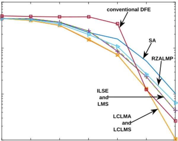
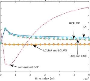
the conventional SA, RLS and LMS algorithms. We emphasize that all of these algorithms are designed to combat the impulsive noise through minimization of different cost functions summarized in Table 5.2. For the sake of clarity, we demonstrate the results of each experiment in two different plots, one for the first order algorithms, i.e., LCLMA, LCLMS, LMS, SA, ILSE, RZALMP and another for the second order algorithms, i.e., LCRLA, LCRLS, RLS and l0-RLS. We have

also provided the complexity comparisons of different methods in Table 5.3. As shown in the Figs. 5.2 and 5.3, our algorithms outperform all other al-gorithms in all SNR values. Also, observe that the conventional DFE cannot perform well in lower SNRs, while in high SNRs, it delivers a comparable perfor-mance to our methods. Moreover, the Figs. 5.4 and 5.5 depict the MSE results for the first order and second order algorithms over time at SNR = 20dB, respec-tively (One can observe the MSE comparison at first time steps in Figs. 5.6 and 5.7). Again, the MSE results in Figs. 5.4 and 5.5, show how our algorithms can successfully track the channel variations in this highly non-stationary and im-pulsive noise environment, yielding a superior performance related to the other competitors.

Algorithm Cost function SA |em| LMS |em|2 LCLMS |em|2− 1_aln(1 + a|em|2) LCLMA |em| − 1_aln(1 + a|em|) ILSE 1_λcosh(λem) RZALMP |em|p+ λ L ∑ i=1 log(1 +|ˆhi| δ ) RLS m ∑ i=1 λm−i|ei|2 LCRLS m ∑ i=1 λm−i|ei|2−_a1ln(1 + a m ∑ i=1 λm−i|ei|2) LCRLA m ∑ i=1 λm−i_|e i| −_a1ln(1 + a m ∑ i=1 λm−i_|e i|) l0-RLS m ∑ i=0 λm−i|e i|2+ ζ∥ˆhn∥0, where ∥ˆhn∥0 ≈ K∑−1 k=0 (1− exp(−η|ˆhk|))

Table 5.2: Cost functions of the competing algorithms.

Algorithm × + / sign SA 2L 2L 1 LMS 2L + 1 2L LCLMS 2L + 5 2L + 1 1 LCLMA 2L + 3 2L + 1 1 1 ILSE L + M + 2 L + N + 1 1 RZALMP 3L + M + 1 3L + N L L + 1 RLS 4L2+ 3L 3L2+ L L + 1 LCRLS 4L2_{+ 4L + 3 3L}2_{+ L + 1 L + 2} LCRLA 4L2_{+ 4L + 2 3L}2_{+ L + 1 L + 2 1} l0-RLS 7L2+ 6L + LM + 2 6L2 + LN + 1 L + 3 L

Table 5.3: Computational complexity comparison of different algorithms. Number of each operation (on real numbers) needed by different algorithms per one sample processing is pro-vided in the table. We have assumed that the exponentiating to a non-integer number needs

M multiplication and N additions. As we see in this table without any significant increase

in the computational complexity, compared to the traditional methods we obtain a superior performance.

Eb/N0(dB) 0 5 10 15 20 25 30 BER 10-3 10-2 10-1 100 BER vs. SNR conventional DFE SA RZALMP LCLMA and LCLMS ILSE and LMS

Figure 5.2: BER vs SNR of the first order algorithms, in a 5% impulsive noise environment. This figure shows the superior performance of LCLMS and LCLMA algorithms. Eb/N0(dB) 0 5 10 15 20 25 30 BER 10-3 10-2 10-1 100 BER vs. SNR LCRLS LCRLA RLS LZRLS conventional DFE

Figure 5.3: BER vs SNR of the second order algorithms, in a 5% impulsive noise environment. This figure shows the superior performance of LCRLS algorithm.

time index (m) ×104

0 1 2 3 4 5 6

Mean Squared Error

0.4 0.5 0.6 0.7 0.8 0.9 1 1.1 1.2 1.3 1.4

MSE performance comparison at SNR = 20dB

conventional DFE

LCLMA and LCLMS

SA

LMS and ILSE RZALMP

Figure 5.4: MSE of the first order algorithms, in 5% impulsive noise environ-ment. This figure shows the superior convergence performance of the LCLMS and LCLMA methods at SNR = 20 dB.

time index (m) _×104

0 1 2 3 4 5 6

Mean Squared Error

0.4 0.5 0.6 0.7 0.8 0.9 1 1.1 1.2 1.3

1.4 MSE performance comparison at SNR = 20dB conventional DFE

LCRLS LZRLS

RLS and LCRLA

Figure 5.5: MSE of the second order algorithms, in 5% impulsive noise environ-ment. This figure shows the superior convergence performance of the LCRLS method at SNR = 20 dB.

time index (m)

0 1000 2000 3000 4000 5000 6000 7000 8000 9000 10000

Mean Squared Error

0.4 0.5 0.6 0.7 0.8 0.9 1

1.1 MSE performance comparison at SNR = 20dB

conventional DFE LCLMA and LCLMS

SA RZALMP

LMS and ILSE

Figure 5.6: MSE comparison for different first order methods.

time index (m)

0 1000 2000 3000 4000 5000 6000 7000 8000 9000 10000

Mean Squared Error

0.8 0.85 0.9 0.95 1 1.05

MSE performance comparison at SNR = 20dB

LCRLS LCRLA RLS LZRLS

ν_i 0.01 0.02 0.03 0.04 0.05 0.06 0.07 0.08 0.09 0.1 0.11 BER 10-3 10-2 10-1 100

BER for different ν_i values

LCLMA conventional DFE LMS and ILSE RZALMP LCLMS SA

Figure 5.8: BER at different impulse probabilities for the first order algorithms. The experiments are done at SNR= 20 dB.

ν_i 0.01 0.02 0.03 0.04 0.05 0.06 0.07 0.08 0.09 0.1 0.11 BER 10-3 10-2 10-1 100

BER for different ν_i 's

LCRLS LCRSA RLS LZRLS conventional DFE

Figure 5.9: BER at different impulse probabilities for the second order algorithms. The experiments are done at SNR= 20 dB.

We also investigate the effect of the impulse probability, νi, on the

perfor-mance of the proposed algorithms. To this end, we set the SNR to 20 dB and obtain the BER at different impulse probabilities, as shown in Figs. 5.8 and 5.9. Based on these simulations, when the impulse probability increases, our algorithms significantly outperform other methods. This superior performance

makes our algorithms suitable candidates for the highly impulsive noise real life channels.

5.3

Conclusion

In this thesis, we presented a novel family of linear channel estimation algorithms based on the logarithmic cost functions. Specifically, we introduce two first or-der methods, i.e., LCLMA and LCLMS, as well as two second oror-der methods, i.e., LCRLA and LCRLS, as robust adaptive estimators for underwater acous-tic channels. We implement these algorithms in a decision feedback equalization framework and remove the ISI in two consecutive stages, i.e., a channel estimation based equalizer followed by a blind equalizer. Our methods achieve a comparable convergence rate to the algorithms seeking to minimize higher order norms of the error, while maintaining the same stability of the lower order norm methods, with similar computational complexity to the conventional methods. We provide the tracking and steady-state performance analysis of the proposed algorithms both in the impulse-free and impulsive noise environments, in the presence of frequency and phase offsets, which are among the common impairments in un-derwater acoustic communications. Finally, we show the enhanced performance of the new algorithms in a highly realistic UWA communication scenario.

Bibliography

[1] P. Qarabaqi and M. Stojanovic, “Statistical characterization and computa-tionally efficient modeling of a class of underwater acoustic communication channels,” IEEE J. Ocean. Eng., vol. 38, no. 4, pp. 701–717, 2013.

[2] M. K. Banavar, J. J. Zhang, B. Chakraborty, H. Kwon, Y. Li, H. Jiang, A. Spanias, C. Tepedelenlioglu, C. Chakrabarti, and A. Papandreou-Suppappola, “An overview of recent advances on distributed and agile sensing algorithms and implementation,” Digital Signal Processing, vol. 39, pp. 1–14, 2015.

[3] A. Gunes and M. B. Guldogan, “Joint underwater target detection and track-ing with the bernoulli filter ustrack-ing an acoustic vector sensor,” Digital Signal Processing, vol. 48, pp. 246–258, 2016.

[4] A. C. Singer, J. K. Nelson, and S. S. Kozat, “Signal processing for under-water acoustic communications,” IEEE Communications Magazine, vol. 47, pp. 90–96, January 2009.

[5] D. B. Kilfoyle and A. B. Baggeroer, “The state of the art in underwater acoustic telemetry,” Oceanic Engineering, IEEE Journal of, vol. 25, no. 1, pp. 4–27, 2000.

[6] M. Stojanovic and J. Preisig, “Underwater acoustic communication chan-nels: Propagation models and statistical characterization,” IEEE Commu-nications Magazine, vol. 47, pp. 84–89, January 2009.

[7] D. Peng, Y. Xiang, H. Trinh, and Z. Man, “Adaptive blind equalization of time-varying simo systems driven by qpsk inputs,” Digit. Signal Process., vol. 23, pp. 268–274, Jan. 2013.

[8] J. G. Proakis, Digital Communications. McGraw-Hill, 1995. [9] T. Wong and T. Lok, “Theory of Digital Communications,” 2017.

[10] A. Song and M. Badiey, “Generalized equalization for underwater acoustic communications,” Proceedings of OCEANS 2005 MTS/IEEE, pp. 1522 – 1527, 2005.

[11] Y. R. Zheng and V. H. Nascimento, “Two variable step-size adaptive algo-rithms for non-gaussian interference environment using fractionally lower-order moment minimization,” Digital Signal Processing, vol. 23, no. 3, pp. 831–844, 2013.

[12] X. Xu, S. Zhou, H. Sun, A. K. Morozov, and Y. Zhang, “Impulsive noise suppression in per-survivor processing based dsss systems,” Oceans - St. John’s, 2014, pp. 1–5, September 2014.

[13] S. Banerjee and M. Agrawal, “Underwater acoustic communication in the presence of heavy-tailed impulsive noise with bi-parameter cauchy-gaussian mixture model,” Ocean Electronics (SYMPOL), 2013, pp. 1–7, October 2013.

[14] S. Banerjee and M. Agrawal, “Underwater acoustic noise with generalized gaussian statistics: Effects on error performance,” OCEANS - Bergen, 2013 MTS/IEEE, pp. 1–8, June 2013.

[15] S. Banerjee and M. Agrawal, “On the performance of underwater commu-nication system in noise with gaussian mixture statistics,” 2014 Twentieth National Conference on Communications (NCC), pp. 1–6, March 2014. [16] T. Y. Min and M. Chitre, “Localization of impulsive sources in the ocean

using the method of images,” Oceans - St. John’s, 2014, pp. 1–6, September 2014.

[17] D. Zha and T. Qiu, “Underwater sources location in non-gaussian impulsive noise environments,” Digital Signal Processing, vol. 16, no. 2, pp. 149–163, 2006.

[18] J. He and Z. Liu, “Underwater acoustic azimuth and elevation angle estima-tion using spatial invariance of two identically oriented vector hydrophones at unknown locations in impulsive noise,” Digit. Signal Process., vol. 19, pp. 452–462, May 2009.

[19] J. Zhang and Y. Pang, “Pipelined robust m-estimate adaptive second-order volterra filter against impulsive noise,” Digital Signal Processing, vol. 26, pp. 71–80, 2014.

[20] J. A. Hildebrand, “Anthropogenic and natural sources of ambient noise in the ocean,” Inter-Research, Marine Ecology Progress Series (MEPS), vol. 395, pp. 5–20, December 2009.

[21] H.-Y. Cheng and A.-Y. A. Wu, “Unified low-complexity decision feedback equalizer with adjustable double radius constraint,” Digit. Signal Process., vol. 51, pp. 82–91, Apr. 2016.

[22] Z. Madadi, G. V. Anand, and A. B. Premkumar, “Three-dimensional lo-calization of multiple acoustic sources in shallow ocean with non-gaussian noise,” Digit. Signal Process., vol. 32, pp. 85–99, Sept. 2014.

[23] M. U. Otaru, A. Zerguine, and L. Cheded, “Channel equalization using sim-plified least mean-fourth algorithm,” Digital Signal Processing, vol. 21, no. 3, pp. 447–465, 2011.

[24] A. Zerguine, “Convergence and steady-state analysis of the normalized least mean fourth algorithm,” Digit. Signal Process., vol. 17, pp. 17–31, Jan. 2007. [25] M. O. Sayin, N. D. Vanli, and S. S. Kozat, “A novel family of adaptive filtering algorithms based on the logarithmic cost,” Signal Processing, IEEE Transactions on, vol. 62, pp. 4411 – 4424, September 2014.

[26] S. Haykin, Adaptive filter theory, 4th edition. Prentice Hall information and system sciences series, Upper Saddle River, N.J. Prentice Hall, 2002.