THE EFFECT OF OIL CONSUMPTION ON ECONOMIC
GROWTH IN TURKEY
TÜRKİYE’DE PETROL TÜKETİMİNİN EKONOMİK BÜYÜMEYE ETKİSİ
Harun TERZİ
(1), Uğur Korkut PATA
(2)(1, 2) Karadeniz Teknik Üniversitesi, İİBF, İktisat Bölümü (1) [email protected]; (2) [email protected] Geliş/Received: 08-02-2016, Kabul/Accepted: 26-06-2016
ABSTRACT: This study investigates the causality link between economic growth and oil consumption using annual data over the years of 1974-2014 by using causality tests and the Engle-Granger and Gregory-Hansen co-integration models for the Turkish economy. The empirical findings support the view that there is no long term co-integration between the level of economic growth and oil consumption level. However, the UVAR, TYVAR and Hsiao’s Granger causality tests in the short term show that a positive one-way causality is going from the oil consumption level to the economic growth rate, and oil consumption level stimulates economic growth rate. Keywords: Energy Consumption, Oil, Economic Growth, VAR Analysis, Turkey JEL Classifications: Q43, C32
ÖZ: Bu çalışmada 1974-2014 dönemi yıllık verilerle Türkiye ekonomisi için ekonomik
büyüme ile petrol tüketimi arasındaki ilişkiler kısa dönem nedensellik testleri, uzun dönem Engle-Granger ve Gregory-Hansen eşbütünleşme yöntemleri ile incelenmiştir. Ampirik sonuçlar değişkenler arasında uzun dönemde eşbütünleşme ilişkisinin olmadığını, ancak UVAR, TYVAR ve Hsiao’nun Granger nedensellik testleri kısa dönemde petrol tüketiminden ekonomik büyümeye doğru pozitif, tek yönlü bir nedenselliğin olduğunu, petrol tüketimi arttıkça büyüme hızının arttığını göstermektedir.
Anahtar Kelimeler: Enerji Tüketimi, Petrol, Ekonomik Büyüme, VAR Analizi, Türkiye
1. Introduction
The industrial revolution after 1850 has generated modern production methods based on energy (oil), and oil has played an important role throughout in the industrialization process. After the great depression in 1929 considered as the deepest economic depression of the 20th century, the 1973 (first oil shock) and 1979 (second oil shock)
crises have caused massive shortages and dramatic negative impact on oil dependent (intensive) countries (industries). The oil crises called as a halt to global economic development and hit heavy industries all over the world seriously. In macroeconomic sense, industrialized countries started to shift alternative and new energy sources to decrease oil dependency, especially in the heavy industries. However, at the present many countries’ oil dependency is rapidly increasing and oil still has an important share in total energy consumption, accounted for 37 (and 32) % of energy consumption in 1990 (and 2010 respectively). In the last 20 years, the share of oil in total energy consumption has changed very little. It is a common view in the growth literature that oil production/consumption and oil price have a considerable impact on future economic growth rate. The historical time series data indicates that after a shock
increase in the oil price, employment rate, industrial production and other economic activities start to decrease after a time lag.
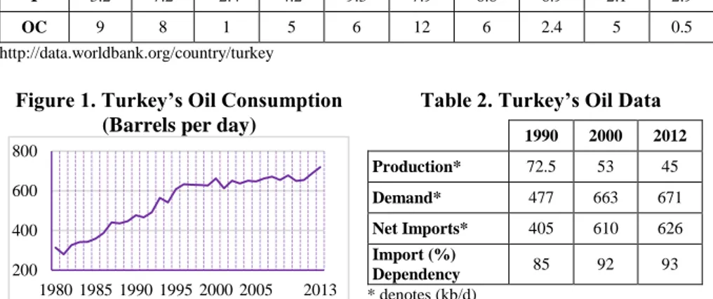
Many empirical studies in both developing and developed countries support the view that a decrease in oil consumption/production or an increase in oil price causes a decrease in growth rate and economic activities. The studies concerning the relationship between the crude oil price and GDP growth in the global level indicate that the spikes in oil price were caused a sharp and rapid decrease in the global economic growth rate, and it is still considered as a threat to economic stability and development (Difiglio, 2014: 50). Some studies concluded that the spikes in oil price generate recession, especially in the transportation, vehicles sectors, and many industries over the following years. It is also noted that many studies just emphasized the role of capital and labor in economic growth but ignored the role of energy factor such as oil, natural gas and electricity in the production function. This weak point can be eliminated by including energy in the production function to make the estimated results more reliable. Yoo (2006) came to the conclusion that oil is a closely interrelated and complementary factor to labor and capital. The productivity level of other production factors is also strongly affected by the fall of the oil production. In the last decades, Turkey as a developing country has had a steadily growing rate, and fast oil demand increased in all sectors. The growth rate of the Turkish economy is an average of 4.2 (4.3) % annually from 1980 to 2014 (1990-2014). In the 25 years before the global economic crisis in 1999, Turkey’s GDP grew 4.5% on average annual variation per year. After 1999, Turkey’s average GDP growth rate per year is 5.8% (except the 2001 and 2009 economic crises), still less than a double-digit as shown in Table 1. In parallel with economic growth, it seems that oil/energy consumption has been growing in line with economic growth. Oil consumption accounts for 28% of the total energy consumption in 2013. According to the Turkish Oil and Natural Gas Sector Report (TPAO) (2015), it is estimated that the oil consumption will account for 26% of total energy consumption until the year of 2023. Crude oil consumption of Turkey in million metric tons drastically increased from 22 in 1990 to 34 in 2014. According to the EIA Report (2015), Turkey has limited oil reserves, and its expanded demand for oil from international markets has increased continuously in the last 20 years. Turkey, like many non-oil producing developing countries, needs more oil to sustain its economic development. Figure 1 shows that oil consumption (OC) has started to increase from 314 in 1980 to 608 in 1995. In comparison with 1980, the annual oil consumption of a thousand barrels in Turkey has risen by 129% and climbed to 719 thousand barrels per day in 2013. After 1980, Turkey become a dependent country on oil imports and its oil consumption/imports increased over time, as shown in Figure 1. Table 2 shows that the oil dependency ratio of Turkey increased from 85% in 1990 to 93% in 2012, and is estimated to be 94% in 2018. The production/consumption ratio was around 6-8% for the period of 2000-2013. While Turkey’s domestic oil production declined, consumption of oil levels slightly continued to increase. In 2002, national oil production consisted of about 7% of total consumption, and transport sector accounted for 50% of total oil consumption. Therefore, oil is one of the main energy inputs in Turkey, and generally considered as one of the key factors to speed up economic growth. The annual rate of increase in oil consumption was 2.7% on average between 1980 and 2013.
In the Indexmundi (2015), Turkey’s oil consumption (oil importing) level in 2014 was 724 thousand barrels daily ranked 26th (25th) highest, however, 90% of oil consumed in
Turkey was imported from foreign countries. Turkey’s annual growth rate of oil consumption was 2.6 percent over the years of 1974-2014. The country was increasingly reliant on oil imports in order to satisfy domestic demand. Turkey’s imports of oil (476) exceeded production by some 430 thousand b/d in 2004. For the period of 2004-2014 (thousand b/d in annual average), while oil production 46.5, oil import was 369. The economic growth has boosted the oil consumption, which has doubled in the last 30 years. Many consider oil dependency is the primary source for current account deficit (CAD) in oil importing countries. In terms of CAD, Turkey reached the upper level among the developing economies. Turkey’s CAD amounted to -7.7 (-5.5) % of GDP at the end of 2013 (2014). Some studies in Turkey have shown that country is mainly dependent on oil imports for its growing economy, but energy-oil dependency also increases CAD. Oil imports have significant positive impact on CAD (e.g., Ozata, 2003). Therefore, the decline in oil price and expense also helps to reduce the deficit. There are few studies focusing on the response of the economic growth rate to the consumption level of oil. Therefore, this study is intended to offer an extensive analysis on the causality link between the consumption level of oil and the economic growth rate.
Table 1. GDP (Y) and Oil Consumption (OC) Annual Growth Rate (%)
1970 1975 1980 1985 1990 1995 2000 2006 2012 2014
Y 3.2 7.2 -2.4 4.2 9.3 7.9 6.8 6.9 2.1 2.9
OC 9 8 1 5 6 12 6 2.4 5 0.5
http://data.worldbank.org/country/turkey Figure 1. Turkey’s Oil Consumption
(Barrels per day)
Table 2. Turkey’s Oil Data
1990 2000 2012 Production* 72.5 53 45 Demand* 477 663 671 Net Imports* 405 610 626 Import (%) Dependency 85 92 93 * denotes (kb/d)
In this study, 5 sections are organized as follows; section 1 shortly points out the importance of oil consumption in the Turkish economy; section 2 presents empirical results from the country’s experiences; section 3 explains time series data and briefly presents econometric methods, section 4 summarizes findings of time series analyses and finally, section 5 presents a summary of the findings, and possible direction for the next studies.
2. Literature Review
In the last 20 years, many empirical studies regarding the relationship between consumption level of oil/energy and growth rate of economics have been presented. In the literature review of this work, 13 studies are based on bivariate causality models, and just 3 studies are based on multivariate causality models. It is generally accepted in the causality models that the association between oil/energy consumption levels and the economic growth rate are statistically significant. But,
200 400 600 800
there is no any common result regarding the way of the causality. While some studies support the view that there is a two-way (feedback) causality, some studies support the argument that there is only a one-way causality. The results of empirical findings based on different time periods and methodologies are not the same. Despite the increasing number of the causality studies concerning the causality link between electricity/coal/natural gas consumption and economic growth, there are limited studies analyzing the causality link between economic growth and oil consumption. The basic findings of earlier studies in the recent literature are summarized as follows:
Yang (2000) examined the causality between two variables, economic growth and oil consumption in the Granger sense, by utilizing annual data over the years of 1954-1997 in Taiwan, and concluded that the direction of causality is going from economic growth rate to oil consumption level. Ageel and Butt (2001) investigated the causality relation between economic activity and oil consumption by employing per capita annual data over the years of 1955-1996 in Pakistan by utilizing the EG co-integration test and the Hsiao’s version of the Granger causality test based on the FPE. They concluded that there is no co-integration, but in the short term economic growth leads to growth in oil consumption. Lee and Chang (2005) studied co-integration and Granger causality link between economic growth and oil consumption by employing annual data over the years of 1954-2003 in Taiwan. They found that a one-way causality is moving from consumption level of oil to economic growth rate. Mostly studies conclude that oil is a basic input to sustain economic development in the long period. Yoo (2006) investigated causality link between economic growth and oil consumption employing annual data over the years of 1968-2002 for the Korean economy by utilizing the co-integration, Granger causality tests and VECM. He concluded that there is a two-way causality between two variables. Economic growth and oil consumption directly affect and stimulate each other with feedback.
Zou and Chau (2006) analyzed the causality link between economic growth and oil consumption for China employing annual data over the years of 1978-2000, (23 observations) by employing co-integration test and ECM. They concluded that series having equilibrium relations are co-integrated, and oil consumption has a causality effect on growth in the short and long terms. Aktas and Yılmaz (2008) examined the causality relations between economic growth and oil consumption for the Turkish economy and employed annual data over the years of 1970-2004 by utilizing the JJ co-integration, Granger causality tests and ECM. They concluded that two variables have a two-way causality both in the short and long terms, therefore, the level of oil consumption has an important impact on the level of employment and income.
Yuan, Kang, Zhao and Hu (2008) examined the causality relations between economic growth and oil consumption in China employing annual data over the years of 1963-2005 by utilizing the JJ co-integration, Granger causality tests and ECM. They concluded that there exists a long-term co-integration between the variables, and Granger causality is going from oil consumption to GDP in the long term, from GDP to oil consumption in the short term. Bhusal (2010) used annual data from 1975-2009 to estimate feedback relationship between economic growth and oil consumption for Nepal employing the Granger causality test. He found that
there is a two-way causality between economic growth and oil consumption in the both short and long terms. Therefore, oil consumption is an important input for the Nepal’s economic growth. Kocaslan and Yılancı (2010) examined causality between economic growth (real GDP 2010=100) and oil consumption (million tons) in Turkey by employing JJ co-integration and VEC models with annual data over the years of 1970-2007. They concluded that the negative causality effect is going from oil consumption to economic growth in the long term, and there is no causality in the short term, therefore oil consumption decreases economic growth in the long term.
Fuinhas and Marques (2012) examined causality between economic growth and oil consumption in Portugal by employing the ARDL and UEC models with annual data over the years of 1965-2008. They concluded that there is a two-way causality between consumption levels of oil and economic growth rate both in the short and long terms. Bhattacharya and Bhattacharya (2014) analyzed the causality relationship between economic growth and petroleum consumption for the two most developing nations, India and China in a VECM framework with annual data over the years of 1980-2010. Their findings suggest that there is a one-way causality from consumption of oil to economic growth in case of India and China in both the short and long terms.
Nasiru, Usman and Saidu (2014) analyzed the causality relationship between consumption level of oil and economic growth in Nigeria by applying the Granger causality and co-integration procedures with annual data over the years of 1980-2011, and concluded that consumption level of oil has no long term relationship with the economic growth rate, but the Granger causality test revealed that a one-way causality is going from consumption level of oil to economic growth. Park and Yoo (2014) investigated the causality link between economic growth and consumption level of oil in Malaysia by employing the Granger causality, co-integration and VEC methods with annual data over the years of 1965-2011, and concluded that there is a two-way causality both in the short and long terms, therefore, an increase in consumption level of oil directly affects economic growth. Stambuli (2014) analyzed the links of causality relationship between growth rate of GDP and consumption level of oil in Tanzania by employing the Granger causality and co-integration tests with annual data over the years of 1972-2010, and concluded that variables are co-integrated and there is a one-way causality going from real GDP to consumption level of oil. Therefore, reduction of consumption levels of oil has no negative effect on economic growth.
Sanlı and Tuna (2014) analyzed the association between economic growth and consumption level of oil employing annual data over the years of 1980-2011 in Turkey. They employed the Granger causality and co-integration procedures, and found no co-integration and causality relationship. Lach (2015) studied causality relations between consumption level of oil and economic growth using quarterly data over the years from 2000q1 to 2009q4 in Poland by the application of error term based on bootstrap, nonlinear causality, TYVAR causality and VEC methods, and concluded that consumption level of oil causes economic growth in the short term, however, causality runs the opposite direction in the long term.
3. Variables and Methodology
This study covers the availability of annual time series data of Turkey oil consumption and economic growth (OCB, OC) rate Y- from 1974 to 2014 after the oil crisis period. The consumption level of oil data -OCB (total oil consumption, thousand barrels per year) and OC (oil consumption million tons per year)- where obtained from the BP World Energy Statistics (2015), and economic growth variable real GDP –Y (expressed in constant 2009 US dollars)- was obtained from the World Bank’s WDI online data set. Three variables consisting of 41 observations are expressed in the logarithmic terms, and following econometric programs, eviews, microfit, rats, gretl and tsp are employed. In this study, econometric models are described shortly and skipped the detailed theoretical description to save space. In this study, firstly traditional and extended version of the Dickey-Fuller (ADF) (1981) and Phillips-Perron (PP) (1988, 1989) unit root tests, and then the Lumsdaine-Papell (LP) (1997) and Lee-Strazicich (LS) (2003) unit root tests considering structural breaks in the series have been applied to examine the stationarity and order of integration in the selected variables before running the alternative causality tests. The ADF test bases on a parametric AR structure, but the PP test bases on a nonparametric correction and the possibility of a structural break in data, therefore two tests treat serial correlation differently. According to Davidson and MacKinnon (2001), the ADF tests perform better than the PP tests in small samples.
The most common utilized stationary tests, having the same h0 and h1 hypotheses
are formulated in equations (1), (2) and (3). Model 1 contains neither constant nor time trend (both are insignificant), model 2 omits time trend, but contains constant, and model 3 contains both constant and time trend. The lags in the ADF and PP tests are selected according to the Bayesian information criterion (BIC). In the following three equations, ADF and PP tests examine the h0 hypothesis of =0 (unit
root) against the h1 hypothesis of <0 (no unit root). is the first difference of the
series, 0 is a constant, 1 is the coefficient of the variable of time trend, I is the
coefficient of the lagged dependent variable, Yt is the time series data, t is the
variable of time trend, m is the number of lags added to ensure that the error terms () are white noise. If the calculated t value of the lagged Yt coefficient (I) which
in absolute terms is greater than the table values listed in MacKinnon (1992), Y is stationary.
∆Yt=δYt-1+ωI∑ ∆Ym t-I
I=1 +εt Model A (1)
∆Yt=β0+δYt-1+ωI∑ ∆YmI=1 t-I+εt Model B (2)
∆Yt=β0+β1t+δYt-1+ωI∑ ∆YmI=1 t-I+εt Model C (3)
The PP and ADF unit root tests do not consider the effect of the structural breaks. If series have one or more structural break, these unit root tests cannot give reliable results. Therefore, this study also employs Lumsdaine Papell (LP) (1997) and Lee-Strazicich (LS) (2003), namely LM unit root test with two structural breaks unit root tests. LP unit root test bases on two equations (models). Model AA allows a two- time change in the level series; Model CC combines two-time changes both in the intercept and the slope of the trend function (Lumsdaine & Papell, 1997: 215).
∆Yt = +βt+θyt-i+φ1DU1t+ω1DT1+ ∑mi=1di∆Yt-i+ut Model AA (4)
∆Yt = +βt+θyt-i+φ1DU1t+ω1DT1+φ2DU2t+ω2DT2+ ∑mi=1di∆Yt-i+ut Model CC
(5)
In the models the first break date is TB1, the second break date is TB2, if t>TB1(TB2), DU1(DU2) =1, otherwise 0. If t>TB1(TB2), DT1(DT2) = TB1(TB2) otherwise similarly 0. H0:
θ
=0 hypothesis in the models AA and BB shows that thedata has a unit root with a drift that excludes any structural break. H1:
θ
<0hypothesis implies that the variable has a trend-stationary process with a two-time break occurring at an unknown point in time. LS unit root test differs from LP unit root test in h0 hypothesis indicating that data has a unit root with two structural
breaks.
Engle-Granger (EG) (1987) developed two steps approach to test long term co-integration relationship which is an error term-based version of the ADF test, but critical values are provided by Engle & Yoo (1987).
The EG test consists of the following steps: Set h0 (=0) and h1 (<0) hypotheses
and estimating the long term equilibrium equation (6) by OLS, then obtaining error term based equations (7) and (8) and applying the ADF test on the error term to see error terms have unit roots or not. If the error terms are stationary at the levels, two variables are said to be co-integrated in the long term.
Yt=β0+ β1XI+ut (6)
∆ut=σ+δut-1+ ∑pI=1αI∆ut-I+φt (7)
∆ut=σ+β1t+δut-1+ ∑pI=1αI∆ut-I+φt (8)
where both Yt and Xt are non-stationary variables and integrated of order one. If Yt
and Xt to be co-integrated, the necessary condition is that the estimated error terms
from the equation (6) should be stationary (utI(0)) according to the ADF test. In
other words, if t-statistics of the coefficient of exceeds the Engle-Yoo’s table values Y and OC/OCB is said to be co-integrated. The EG co-integration test may lose its power if there is a break in co-integration relationship. Gregory-Hansen (GH) (1996) developed a co-integration test, an error term based method, allowing either a break in all coefficients or a break in constant only, or to have a trend or not. In GH co-integration test h0 hypothesis (no co-integration with structural
breaks) is tested against the h1 hypothesis (co-integration with a structural break).
The GH co-integration test presents three alternative models: Model 1 (C): a level shift; Model 2 (C/T): level shift with trend; and Model 3 (C/S): regime shift (allows change in intercept and slope coefficients) for testing co-integration. Models are listed as follows:
Yt = μ1+μ2DUt+α1TXt+ut Model 1 (9)
Yt = μ1+μ2DUt+μ3TXtDUt+α1TX1+ut Model 3 (11)
If the ADF test statistic is smaller than the corresponding table value, the h0
hypothesis is rejected. Several causality methods have been developed in literature. The Hsiao’s Granger causality tests (1981) in equations (12) and (13) is utilized Akaike’s minimum final prediction error (FPE) criteria based on two step procedure whether X causes Y. T is the size of sample, SSE is the squared sum of errors, δ is constant, ϑ and ∂ are coefficients, u1t and u2t are error terms. The first step estimates
lag m according to equation (12), and the FPE(m) value. The second step estimates lag n according to equation (13), and the FPE(m, n) value. If the FPE(m, n)< FPE(m), X causes Y. To test whether Y causes X, the X and Y should be transposed in equations (12) and (13) by repeating the same procedure.
∆Yt= δ + ∑mi=1ϑ∆Yt−i+ u1t FPE(m)=T+m+1T-m-1SSE(m)/T (12)
∆Yt=δ+ ∑mI=1ϑ∆Yt-I+ ∑j=1n ∂∆Xt-j+u2t FPE(m,n)=T+m+n+1T-m-n-1 SSE(m,n)/T (13)
The VAR model developed by Sims (1980) is commonly used to determine dynamic relationships among the variables. In the unrestricted VAR (UVAR) model, based on equations (14) and (15), variables Y and OC in the UVAR model have one equation and each variable depends on its own lagged values as well as on the lagged values of each other variable in the model. The UVAR model estimated in this study is formalized in the equation and matrix form with the optimal lag (3) as follows:
Yt= α10+ ∑pI=1α11Yt-I+ ∑pI=1α12Xt-I+u1t (14)
Xt= α20+ ∑pI=1α21Xt-I+ ∑pI=1α22Yt-I+u1t (15)
In the UVAR estimation, in equation 14 (15) the h0 hypothesis that OC/OCB (Y)
does not cause Y (OC/OCB) is set as: h0: a121 =a122 =a312=0 (a211 =a212 =a213 =0), and
hypothesis is tested by the WALD test. Toda and Yamamoto (1995) developed a non-causality test called as the TYVAR procedure, which can be applied regardless of the properties of time series data and co-integration relationship.
[Yt OCt] = [ α10 α20] + [ a111 a 12 1 a211 a 22 1 ] [ Yt-1 OCt-1] + [ a112 a 12 2 a212 a 22 2 ] [ Yt-2 OCt-2] + [ a113 a 12 3 a213 a223 ] [Yt-3 OCt-3] + [ u1t u2t]
Each Variable, Y and OC, in the TYVAR model has one equation and each variable depends on its own lagged values as well as on the lagged values of each other variable in the model.
In the TYVAR estimation, in equation 16 (17) the h0 hypothesis that OC/OCB (Y)
does not cause Y (OC/OCB) is set as: h0: a121 =a122 =a312=0 (a211 =a212 =a213 =0), and
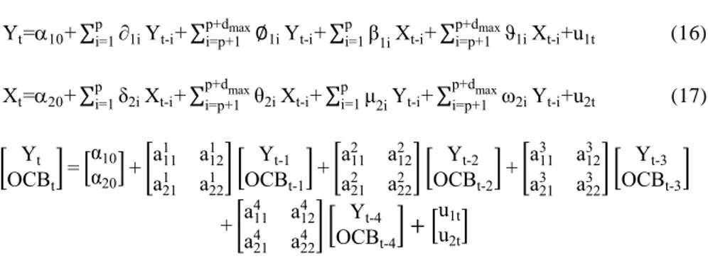
hypothesis is tested by the MWALD test. The TYVAR model estimated in this study is formalized in the equation and matrix form with the optimal lag p+dmax (3+1=4)
Yt=10+ ∑pi=1∂1iYt-i+ ∑p+di=p+1max∅1iYt-i+ ∑pi=1β1iXt-i+ ∑i=p+1p+dmaxϑ1iXt-i+u1t (16)
Xt=20+ ∑pi=1δ2iXt-i+ ∑p+di=p+1maxθ2iXt-i+ ∑pi=1μ2iYt-i+ ∑i=p+1p+dmaxω2iYt-i+u2t (17)
[ Yt OCBt] = [ α10 α20] + [ a111 a 12 1 a211 a 22 1 ] [ Yt-1 OCBt-1] + [ a112 a 12 2 a212 a 22 2 ] [ Yt-2 OCBt-2] + [ a113 a 12 3 a213 a223 ] [ Yt-3 OCBt-3] +[a114 a124 a214 a224 ] [ Yt-4 OCBt-4] + [ u1t u2t]
4. Empirical Results
The descriptive statistics in Table 3 presenting the mean, median, skewness, kurtosis, and the JB values in all three variables indicate that mean and median are close to each other. This implies that the series in the variables are almost symmetric. The p-values of JB test larger than 10% level of significance show that variables have normal distributions. Pearson correlation matrix in Table 4 shows that Y, OCB and OC variables have a positive and strong association as expected. They are going in the same direction, and t statistics of correlation coefficients have a p-value of 0.00 indicating h0 hypothesis is rejected at 1% and two variables are
highly correlated.
Table 3. Descriptive Statistics Table 4. Pearson Correlation Matrix
Variables Y OCB OC Variables Y OCB OC
Mean 9.42 2.69 1.37 Y 1 0.83a 0.83a
Median 9.35 2.75 1.42 OCB 0.83a 1 0.99a
Skewness 0.47 -0.51 -0.48 OC 0.83a 0.99a 1
P-value 0.17 0.11 0.11 a denotes correlations are significant at 1% (2-tailed). Positive correlation corresponds to an increasing relationship.
Kurtosis 1.89 1.74 1.69
J-B 3.60 4.48 4.51
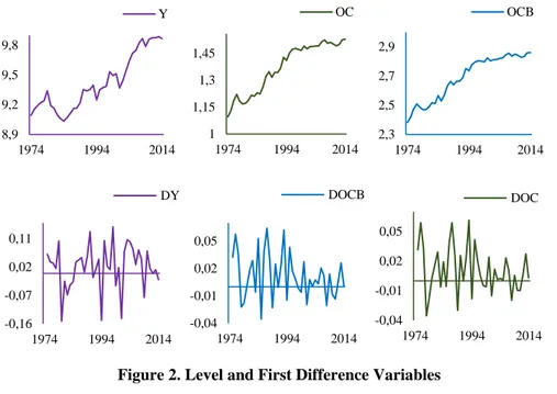
The six series plotted in Figure 2 show that level data having a tendency to drift upwards over time is not stationary, but the first difference are stationary. The unit root tests estimated from the equations (2) and (3) generated the same results. The ADF and PP unit root tests, given in Table 5, show that three variables are not stationary at the level, because the values of ADF and PP tests are less than the table values.
However, for the first difference data h0 hypothesis of non-stationary is rejected at
the 1% level of significance, and variables are integrated of the same level, 1. The unit root tests indicated that variables are appropriate for the econometric techniques used in this study.
Figure 2. Level and First Difference Variables Table 5. ADF and PP Unit Root Tests
ADF Test PP Test
Variables [C] (C+T) [C] (C+T) Y -0.39(0) -2.07(0) -0.37(2) -2.13(2) OCB -1.89(0) -1.63(0) -2.10(6) -1.70(1) OC -1.89(0) -1.61(0) -2.28(4) -1.61(0) ∆Y -6.70(0)a -6.70(0)a -6.70(1)a -6.70(0)a ∆OCB -5.86(0)a -6.00(0)a -5.92(5)a -6.49(9)a ∆OC -6.68(0)a -6.98(0)a -6.74(3)a -7.46(6)a
C: constant, C+T: constant and trend. a indicates that h
0 hypothesis can be rejected at the 1%. Optimal lags are in parentheses selected by the BIC. MacKinnon’s (1991) table values rejecting of h0 hypothesis of a unit root at 1% and 5% in both tests are [-3.61], (-4.20) and [-2.94] (-3.52). The optimal lag length is selected by the Newey-West automatic bandwidth selection method in the PP test.
Table 6. Lumsdaine-Papell Unit Root Test
Variables Model AA p Model CC p
Y -5.28 1979; 2002 0 -4.77 1979; 2003 0 OC -5.68 1985; 1992 0 -5.72 1986; 1992 0 OCB -5.51 1986; 1992 0 -6.12 1986; 1994 0 ∆Y -8.10a 1984; 2002 0 -8.73a 1984; 2002 0 ∆OC -6.40b 1985; 1996 0 -8.09a 1980; 1988 0 ∆OCB -7.30a 1985; 1996 0 -9.21a 1980; 1988 0
Critical values for Model AA (intercept) at 1%: -7.19, 5%: 6.75, 10%: -6.48. Critical values for Model CC (both) at 1%: -6.74, 5%: -6.16, 10%: -5.89. a significant at 1%, b significant at 5%. Optimal lag lengths (p) are selected by the BIC procedure.
8,9 9,2 9,5 9,8 1974 1994 2014 Y 1 1,15 1,3 1,45 1974 1994 2014 OC 2,3 2,5 2,7 2,9 1974 1994 2014 OCB -0,16 -0,07 0,02 0,11 1974 1994 2014 DY -0,04 -0,01 0,02 0,05 1974 1994 2014 DOCB -0,04 -0,01 0,02 0,05 1974 1994 2014 DOC
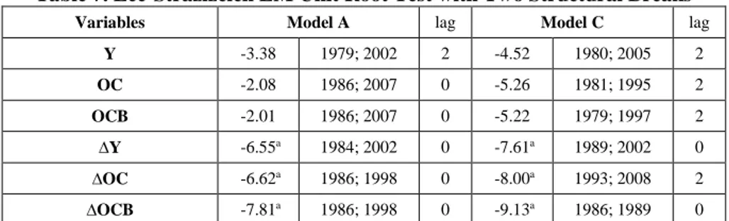
The results of the LP and LS unit root tests listed respectively in Table 6 and Table 7 suggest that the h0 of the unit root hypothesis is rejected for the three variables at least
5% significance level. Therefore, the results of the LS and LP tests confirm the results of both the ADF and PP unit root tests.
Table 7. Lee-Strazizcich LM Unit Root Test with Two Structural Breaks
Variables Model A lag Model C lag
Y -3.38 1979; 2002 2 -4.52 1980; 2005 2 OC -2.08 1986; 2007 0 -5.26 1981; 1995 2 OCB -2.01 1986; 2007 0 -5.22 1979; 1997 2 ∆Y -6.55a 1984; 2002 0 -7.61a 1989; 2002 0 ∆OC -6.62a 1986; 1998 0 -8.00a 1993; 2008 2 ∆OCB -7.81a 1986; 1998 0 -9.13a 1986; 1989 0
Critical values are taken from Lee-Strazicich (2003: p.1084). Critical values for Model A at 1% -4.54, 5% -3.84, 10% -3.50. λ1 denotes the first break, λ2 denotesthesecond break location. λ1 break location respectively 0.17, 0.20, 0.15, 0.4, 0.5 and 0.32. λ2 breaks location 0.73, 0.54, 0.59, 0.70, 0.85 and 0.39. Model C critical values for λ1: 0.2, λ2 : 0.6, 1%: -6.41, 5%: -5.74, 10%: 5.32. Critical values for λ1: 0.2, λ2: 0.8, 1%: -6.33, 5%: -5.71, 10%: -5.33. Critical for λ1: 0.4, λ2: 0.8, 1%: 6.42, 5%: -5.65, 10%: -5.32. Optimal lag lengths (p) are selected by the BIC procedure. a denotes significant at 1%.
The EG co-integration test results shown in Table 8 indicate that the h0 hypothesis
(error terms have unit root) is not rejected at the 10% level. This shows that the error terms of the estimated equations are not stationary in the two equations, therefore, two variables have no relationship, and they do not move together in long term.
Table 8. EG Co-integration Test
Models Error
Terms ADF t-Statistics
Lags by BIC Y=f(OC) u1 -1.38 0 Y=f(OCB) u2 -1.37 0 Y=f(OC) u1 -1.65 0 Y=f(OCB) u2 -1.66 0
Critical values for the EG co-integration test are at 1%, 5% and 10%, 4.32, 3.67 and 3.28 are from Engle-Yoo (1987, p:157) respectively.
Table 9. GH Co-integration Test
Models ADF* t-Statistics Zt* Zα* Break Points (Phillips) Break Points (ADF) Y=f(OC) C -3.37 (3) -3.47 -19.42 2004 2002 C/T -4.51 (0) -4.57 -28.44 1980 1980 C/S -3.70 (7) -3.50 -20.23 1995 1998 Y=f(OCB) C -3.53 (0) -3.69 -21.83 2004 2005 C/T -4.30 (5) -4.51 -28.01 1980 2003 C/S -4.12 (0) -4.21 -25.91 2000 2000
Optimal lag length (froma maximum of 8 lags) is selected by the AIC. Table values at 5% from Gregory-Hansen (1996: p.109) for ADF* and Zt* in Model C, C/T and C/S is -4.61, -4.99 and -4.95. Table values for Zα in Model C, C/T and C/S is -40.48, -47.96 and 47.04, respectively. Break points are selected by the software.
For all possible break points (1974-2014) in GH methods that investigate structural breaks relationship shown in Table 9 indicate that there is no long term co-integration relationship between OC/OCB and Y. ADF*, Zt* and Z* tests do not reject the h0
hypothesis of no co-integration at the 5% level for all models (C, C/T and C/S), and structural breaks are not important in the co-integration relationship.
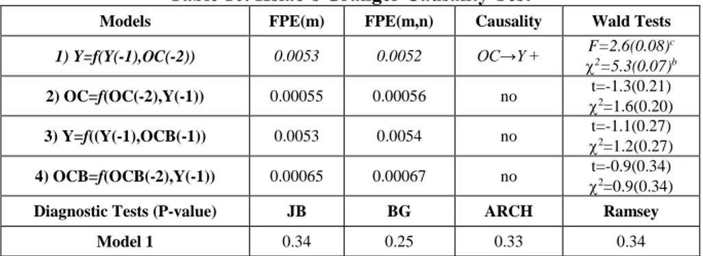
Both the EG two step and the GH procedures do not indicate the existence of a long term movement between Y and OC/OCB. The results of the EG and GH co-integration tests reveal that Y and OC/OCB are not co-integrated. Therefore, the Hsiao’s Granger, UVAR and TYVAR causality tests are applicable to find short term causality. Except the TYVAR model, in conducting the rest of the other causality tests, three variables are transformed into the first difference form. In Table 10, the FPE values (0.0053>0.0052) show a positive one-way causality which in the Granger’s sense is going according to the results of the Hsiao’s Granger causality test.
Table 10. Hsiao’s Granger Causality Test
Models FPE(m) FPE(m,n) Causality Wald Tests
1) Y=f(Y(-1),OC(-2)) 0.0053 0.0052 OC→Y + F=2.6(0.08)2=5.3(0.07)cb
2) OC=f(OC(-2),Y(-1)) 0.00055 0.00056 no t=-1.3(0.21) 2=1.6(0.20)
3) Y=f((Y(-1),OCB(-1)) 0.0053 0.0054 no t=-1.1(0.27) 2=1.2(0.27)
4) OCB=f(OCB(-2),Y(-1)) 0.00065 0.00067 no t=-0.9(0.34) 2=0.9(0.34)
Diagnostic Tests (P-value) JB BG ARCH Ramsey
Model 1 0.34 0.25 0.33 0.34
b and c denote significant at %5 and 10%, respectively.
Table 11. UVAR Causality Analysis
Models 2 Statistics P-value k Causality
Y=f(OC) OC=f(Y) 7.85 1.29 0.05b 0.73 3 OC→Y [+0.89] Yok Y=f(OCB) OCB=f(Y) 6.54 0.97 0.09c 0.81 3 OCB→Y+[1.04] Yok Diagnostic Tests AR Roots max; min LM P-value JB P-value White P-value Model 1 0.61; 0.36 p>0.30 0.29 0.41 Model 2 0.54; 0.41 p>0.41 0.20 0.13
b and c denote significant at 5% and 10%, respectively.
In Table 11, the p-values (0.05 and 0.09) are significant and have positive causality in the Granger’s sense from OC/OCB to Y. The p-values (0.01 and 0.02) are significant and have causality in the Granger’s sense from OC/OCB to Y in Table 12. The sum of the three lags coefficients (1.20 and 1.30) in the TYVAR model is positive and statistically significant according to the Wald test. This result points out that the sign of causality is positive, and a one-way causality is going from OC/OCB to Y. The causality tests show that the inclusion of past values of OC/OCB in the economic growth (Y) equation provides better information regarding Y’s current values than omitting past values of OC/OCB, but not vice versa. Diagnostic tests in the TYVAR and UVAR models imply that the characteristic polynomial AR roots are inside the unit circle, therefore, the model is stable. The p-values of LM, White and JB tests
indicate that there is no indication of the form of the autocorrelation and heteroscedasticity, and error terms have a normal distribution.
Table 12. TYVAR Causality Analysis
Models
2
Statistics P-value p+dmax Causality
Wald Tests (p) Y=f(OC) OC=f(Y) 10.92 2.28 0.01a 0.52 3+1 OC→Y[+1.20]b no F=4.66 p=0.04b Y=f(OCB) OCB=f(Y) 9.80 1.67 0.02b 0.64 3+1 OCB→Y[+1.30]a no F=6.67 p=0.01a Diagnostic Tests AR Roots max; min LM P-value JB P-value White P-value r (e1, e2) Y, OC 0.93; 0.35 p>0.29 0.18 0.60 0.22 Y, OCB 0.95; 0.39 p>0.27 0.17 0.50 0.11
a and b denote significant at 1% and 5%, respectively. Coefficients of error term correlation matrix (r(e1,e2)) are 0.26 and 0.16.
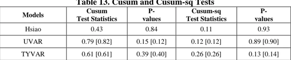
The Cusum and Cusum-sq tests and probability values are presented in Table 13. The results clearly indicate constancy of the coefficients in the five causality models.
Table 13. Cusum and Cusum-sq Tests
Models Cusum Test Statistics P- values Cusum-sq Test Statistics P- values Hsiao 0.43 0.84 0.11 0.93 UVAR 0.79 [0.82] 0.15 [0.12] 0.12 [0.12] 0.89 [0.90] TYVAR 0.61 [0.61] 0.39 [0.40] 0.26 [0.26] 0.13 [0.14]
[ ] values are based on OCB-Y models.
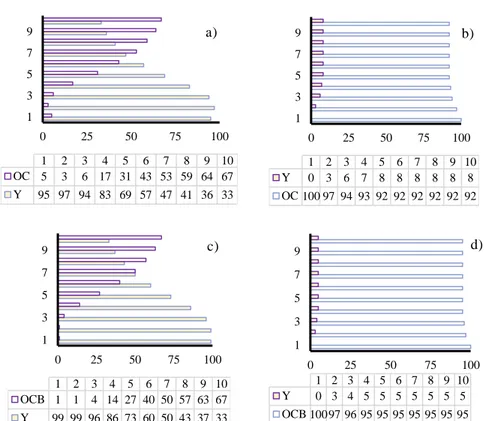
The variance decompositions (VDs) analysis based on the VAR models helps to address the question of causality between OC and Y. The VDs from the UVAR and TYVAR analyses have the same pattern. Therefore, only the results of VDs of TYVAR analysis are presented in Figure 3. The VDs indicate the amount of information from each variable which contributes to the other variables and in the VAR model. In Figure 3a-b, 67% of the variations of Y are explained by OC, while Y accounted for only 8% of shock in OC after ten years. OC explains 35% of variations in Y on ten years’ average. In Figure 3c-d, 67% of the variations of Y are explained by OCB, while Y accounted for only 5% of shock in OCB after ten years. OCB explains almost 32% of variations in Y on ten years’ average. That means the overall results of VDs confirm the findings of the Hsiao’s Granger, the UVAR and TYVAR causality analyses in the long run. This further supports the hypothesis that there is causal effect from oil consumption to Y, and shocks in oil consumption are important to explain economic growth level for at least a ten-year period.
Figure 3. Cholesky Variance Decompositions (VDs)
5. Summary and Conclusions
Whether consumption level of oil affects economic development is one of the important issues in the recent economic literature. In Turkey, oil is one of the main production factors and energy sources for many sectors such as industry, transportation, electricity generation, manufacturing and others. Interestingly, the growth rates of two variables over different time periods have been rather similar. The annual average growth rates of the GDP (at market prices based on constant Turkish Lira) and oil consumption (thousand barrels daily) in Turkey from 1965 to 2014; 1980 to 1990 and 1990 to 2000 are 4.4/4.5; 4.6/4.4 and 4.2/4.1 percentages.
The way of causality relationship between two variables has significant policy implications for policy makers to determine energy policies. In the last decade, several studies examined the causality effect between consumption level of oil and economic growth, but overall results are not conclusive due to the choice of the econometric methods, sample periods and the measure of the variables. The findings of this study are not the same as the findings of previous studies in the Turkish economy. For example, Aktas and Yılmaz (2008) found a positive two-way causality, Kocaslan and Yılancı (2010) reported a negative causality is going from consumption level of oil to economic growth only in the long term, no causality in the short term. Sanlı and Tuna (2014) found that there is no causality relation between the variables in the short and long terms. 0 25 50 75 100 1 3 5 7 9 1 2 3 4 5 6 7 8 9 10 OC 5 3 6 17 31 43 53 59 64 67 Y 95 97 94 83 69 57 47 41 36 33 a) 0 25 50 75 100 1 3 5 7 9 1 2 3 4 5 6 7 8 9 10 Y 0 3 6 7 8 8 8 8 8 8 OC 100 97 94 93 92 92 92 92 92 92 b) 0 25 50 75 100 1 3 5 7 9 1 2 3 4 5 6 7 8 9 10 OCB 1 1 4 14 27 40 50 57 63 67 Y 99 99 96 86 73 60 50 43 37 33 c) 0 25 50 75 100 1 3 5 7 9 1 2 3 4 5 6 7 8 9 10 Y 0 3 4 5 5 5 5 5 5 5 OCB 10097 96 95 95 95 95 95 95 95 d)
This study employs annual Turkish updated data over the years of 1974-2014 after the 1973 oil crises, to investigate whether a causality relationship exists between two variables. The ADF, PP, LP and LS unit root tests show that three variables have no unit roots at the first difference data, the variables are integrated of order Id(1). The EG and GH co-integration test results show that variables are not moving together in the long term. The Hsiao’s Granger causality also indicates that a positive causality is going from OC to Y. In the short term causality analysis, the UVAR and TYVAR analyses show that there is a positive one-way causality going from OC/OCB to Y. The conclusive result from this study is that alternative short term causality methods confirm that increasing consumption level of oil positively affect the economic growth rate in Turkey. Because, a one-way causality is going from only consumption level of oil to economic growth without any feedback effect for the period of 1974-2014. This study based on two-dimensional causality methods commonly used in the empirical literature and diagnostic tests fulfill the linear models’ assumptions and offer the BLUE estimators. The findings in this study point out that the causality link between economic growth rate and consumption levels of oil require more investigation in the future studies by employing alternative bivariate or multivariate models and adding more available variables in the equations.
To sum up, Turkey, as a developing country needs to increase consumption level of oil to speed up its economic growth. The consumption level of oil clearly has a direct impact on the employment and production/service levels on transportation, service and industry sectors. Since a decrease in the oil consumption level causes a decrease in the economic growth rate, therefore, any policy effort to reduce consumption level of oil will generate a negative effect on the economic growth rate.
Turkey has a very limited domestic oil production, and imports almost 90% of oil, and it’s expected that oil demand will increase in coming years. It means that growing oil dependency due to increasing domestic demand may lead to a widening trade/current account deficit. As an abundant country in the renewable energy sources, Turkey must invest more on its renewable sources to reduce oil dependency.
6. References
Aktas, C., & Yilmaz, V. (2008). Causal relationship between economic growth and oil consumption in Turkey. Kocaeli Üniversitesi Sosyal Bilimler Enstitüsü Dergisi, 15(1), 45-55. Ageel, A., & Butt, M. S. (2001). The relationship between energy consumption and economic
growth in Pakistan. Asia-Pacific Development Journal, 8(2), 101-110.
Bhattacharya, M., & Bhattacharya, S. N. (2014). Economic growth and energy consumption nexus in developing world: The case of China and India. Journal of Applied Economics & Business Research, 4 (3), 150-167.
Bhusal, T. P. (2010). Econometric analysis of economic growth and oil consumption in Nepal. Economic Journal of Development Issues, 11, 135-143.
Booth, G. G., & Ciner, C. (2005). German dominance in the European monetary system: A reprise using robust wald tests. Applied Economics Letters, 12(8), 463-466.
British Petroleum. (2015). Statistical review of world energy. Retrieved from http://www.bp .com/content/dam/bp/pdf/energy-economics/statistical-review-2015/bp-stati stical-review-of-world-energy-2015-full-report.pdf
Davidson, R., & Mackinnon, J. G. (2001). Estimation and inference in econometrics., New York: Oxford University Press.
Dickey, D. A., & Fuller, W. A. (1981). Likelihood ratio statistics for an autoregressive time series with a unit root. Econometrica, 49, 1057-1072.
Difiglio, C. (2014). Oil, economic growth and strategic petroleum stocks. Energy Strategy Reviews, 5, 48-58.
Dolado, J. J., & Lutkepohl, H. (1996). Making wald test work for co-integrated VAR systems. Econometric Theory, 15(4), 369-386.
EIA. (2013). Turkey-US energy information administration report. Retrieved from https://www .iea.org/publications/freepublications/publication/2013_Turkey_Country_Chapterfinal_with _last_page.pdf
EIA. (2015). Turkey-US energy information administration report. Retrieved from https://www .eia.gov/beta/international/analysis_includes/countries_long/Turkey/turkey.pdf
Engle, R. F., & Granger, C. W. (1987). Co-integration and error correction: representation, estimation, and testing. Econometrica: Journal of the Econometric Society, 55(2), 251-276. Fuinhas, J. A., & Marques, A. C. (2012). An ARDL approach to the oil and growth nexus:
Portuguese evidence. Energy Sources, Part B: Economics, Planning and Policy, 7(3), 282-291.
Gregory, A. W., & Hansen, B. E. (1996). Residual-based tests for co-integration in models with regime shifts. Journal of Econometrics, 70(1), 99-126.
Hsiao, C. (1981). Autoregressive modelling and money-income causality detection. Journal of Monetary Economics, 7 (1), 85-106.
Kocaslan, G., & Yilanci, V. (2010). Economic growth and oil consumption: Evidence from Turkey. Energy Studies Review, 17(1), 26-32.
Lach, L. (2015). Oil usage, gas consumption and economic growth: Evidence from Poland. Energy Sources, Part B: Economics, Planning, and Policy, 10(3), 223-232.
Lee, C. C., & Chang, C.-P. (2005). Structural breaks, energy consumption, and economic growth revisited: Evidence from Taiwan. Energy Economics. 27(6), 857-872.
Lee, J., & Strazicich, M. C. (2003). Minimum Lagrange multiplier unit root test with two structural breaks. Review of Economics and Statistics, 85(4), 1082-1089.
Lumsdaine, R. L., & Papell, D. H. (1997). Multiple trend breaks and the unit-root hypothesis. Review of Economics and Statistics, 79(2), 212-218.
Nasiru, I., Usman, H. M., & Saidu, A. I. (2014). Economic growth and oil consumption: Evidence from Nigeria. Bulletin of Energy Economics, 2(4), 106-112.
Ozata, E. (2014). Sustainability of current account deficit with high oil prices: Evidence from Turkey. International Journal of Economic Sciences, 3(2), 71-88.
Park, S.-H., & Yoo, S.-H. (2014). The dynamics of economic growth and oil consumption in Malaysia. Energy Policy, 66, 218-223.
Perron, P. (1989). The great crash, the oil price shock, and the unit root hypothesis. Econometrica, 57(6), 1361-1401.
Phillips, P. C. B., & Perron, P. (1988). Testing for unit roots in time series regression. Biometrika, 75(2), 335-346.
Sanli, F. B., & Tuna, K. (2014). Türkiye’de petrol tüketimi ile ekonomik büyüme arasındaki ilişkinin analizi. Maliye Finans Yazıları, 102(28), 43-58.
Sims, C. A. (1980). Macroeconomics and reality. Econometrica, 48 (1), 1-48.
Stambuli, B. B. (2014). Economic growth and oil consumption nexus in Tanzania co-integration causality analysis. International Journal of Academic Research in Economic and Management Sciences, 3(2), 113-123.
TPAO. (2015). Ham petrol ve doğal gaz sektör raporu. Retrieved from http://www.enerji.gov .tr/file/?path=root%2f1%2fdocuments%2fsekt%c3%b6r+raporu%2fhp_dg_sektor_rpr.pdf Yang, H.-Y. (2000). A note on the causal relationship between energy and GDP in Taiwan. Energy
Economics, 22(3), 309-317.
Yoo, S. H. (2006). Economic growth and oil consumption: Evidence from Korea. Energy Sources, 1(3), 235-243.
Yuan, J. H., Kang, J.-G., Zhao, C.-H., & Hu, Z. G. (2008). Energy consumption and economic growth: Evidence from China at both aggregated and disaggregated levels. Energy Economics, 30(6), 3077-3094.
Zou, G. L., & Chau, K. W. (2006). Short-and long-run effects between economic growth and oil consumption in China. Energy Policy, 34(18), 3644-3655.