Electromagnetic scattered field analysis of 2D wedge geometries with HFA techniques and FDTD method

(1)

T.C. DOGUS UNIVERSITY

Institute of Science

ELECTROMAGNETIC SCATTERED FIELD ANALYSIS OF 2D

WEDGE GEOMETRIES WITH HFA TECHNIQUES AND FDTD

METHOD

M.Sc. Thesis

Mehmet Alper USLU

201092004

Thesis Supervisor: Prof.Dr. Levent SEVGI

(2)

(3)

i

ACKNOWLEDGEMENTS

I would like to express my deepest gratitude to my M.Sc. supervisor, Prof. Dr. Levent SEVGI, for his guidance and valuable help throughout the thesis. He provided me with a better understanding of many concepts as well as academic insight. His contributions will effect in the rest of my academic life. He is intelligent supervisor and an excellent person for all aspects.

I would like to thank Prof. Dr. Cem GOKNAR, Prof. Dr. Ergul AKCAKAYA, Prof. Dr. Ercan TOPUZ and Assist. Prof. Dr. Zekeriya UYKAN for their scientific contributions to my academic career.

I would like to also thank Assist. Prof. Dr. Cagatay ULUISIK for countless reasons. Most importantly, he was like a brother to me throughout all my graduate and undergraduate studies in Dogus University in the past 5.5 years. Without his guidance and support I cannot continue my academic career.

I would like to thank my friends and colleagues in Dogus University. My thanks go to Cihan AYDIN, Ozlem UNAN, Onur GUVENC, Bayram CEYHAN and Ahmet SEFER. Finally, my special thanks go to my family for supporting me in every way they can.

(4)

ii

ABSTRACT

In this thesis, electromagnetic scattered field analysis of two dimensional non-penetrable wedge geometry have been investigated with both high frequency asymptotic techniques (HFA) and finite difference time domain (FDTD) method.

Among HFA techniques, Physical optics (PO), Physical theory of diffraction (PTD), Unified theory of diffraction (UTD), Parabolic equation (PE), Exact series and Exact integral methods are applied to inspect electromagnetic scattering behavior of two dimensional non-penetrable wedge geometry analytically.

As a numerical technique, finite difference time domain (FDTD) method and the important aspects in its implementation are explained briefly. Also, absorbing boundary conditions and modeling issues are investigated. Meshing algorithm is developed to reduce staircase modeling errors which is formed by the application of standard Yee algorithm. In order to show the qualification of FDTD method, some examples are presented with HFA results. A novel Matlab based softwares WEDGE GUI and WEDGE FDTD GUI are also presented with thesis. The former was developed to analyze two dimensional perfect electric conductor (PEC) wedge geometries with various HFA methods. The latter was developed to analyze same geometry with finite difference time domain (FDTD) method. Source codes of these programs can be found in the CD given with this thesis.

(5)

iii

ÖZET

Bu tezde, kusursuz iletken yapıdaki üçgensel objelerden oluşan elektromanyetik saçılım alanları, yüksek frekans asimtotik teknikleri ve zaman domeninde sonlu farklar yöntemi ile incelenmiştir.

Yüksek frekans asimtotik tekniklerden, fiziksel optik, fiziksel difraksiyon teorisi, birleştirilmiş difraksiyon teorisi, parabolik denklem, seri ve integral metotları bu tip problemleri analitik olarak analiz etmek için uygulanmıştır.

Bir numerik teknik olan zaman domeninde sonlu farklar metodu ve bu metodun uygulanması da bu tez içerisinde detaylı bir şekilde anlatılmıştır. Yutucu sınır koşulları ve modelleme sorunları da ayrıca incelenmiştir. Standart Yee algorithmasının uygulanmasından dolayı oluşan modelleme hatalarını düşürmek için, hücreleme algorithması geliştirilmiştir. Zaman domeninde sonlu farklar yönetiminin sonunçlarının doğruluğunu göstermek için birkaç örnek yüksek frekans asimtotik yöntemlerinin sonuçları ile birlikte verilmiştir.

Bu tez kapsamında, WEDGE GUI ve WEDGE FDTD GUI adında iki yeni matlab tabanlı program sunulmuştur. WEDGE GUI, 2 boyutlu kusursuz iletken üçgensel objeleri çeşitli yüksek frekans asimtotik teknikler ile kolay bir şekilde analiz etmek için geliştirilmiştir. WEDGE FDTD GUI ise aynı geometriyi zaman domeninde sonlu farklar yöntemi ile analiz etmek için tasarlanmıştır. Bu programların kaynak kodları tez ile birlikte verilen CD içerisinde bulunabilir.

(6)

iv

ABBREVATIONS

Two Dimensional Three Dimensional

Magnetic flux density vector Electric flux density vector

Frequency

Magnetic field intensity vector Imaginary unit

_{Uniform surface currents generated by the incident field} _{Non-uniform surface currents generated by the incident field}

Electric current density vector

Wave vector

Magnetic current density vector

_{Exact solution for the soft ( ) boundary conditions} _{Exact solution for the hard ( ) boundary conditions}

Amplitude of incident field

_{Geometrical optics total fields (sum of the incident and reflected} fields)

_{Diffracted fields (i.e., exact total field solution minus the Geometrical} Optics fields)

_{Physical Optics total fields}

_{Physical Theory of Diffraction total fields}

_{Physical Optics diffracted fields (i.e. Physical optics total fields minus} the Geometric Optics fields)

_{Physical Theory of Diffraction diffracted fields (i.e. Physical Theory} of Diffraction total fields minus the Geometric Optics fields)

Gradient

Curl

Electrical permittivity

Relative electrical permittivity Magnetic permeability

Electrical conductivity Wave angular frequency

(8)

vi ABC Absorbing boundary condition

CFDTD Conformal finite difference time domain FDTD Finite difference time domain

PML Perfectly matched layer

(9)

vii

LIST OF FIGURES

Figure 2.1 Geometry of the wedge scattering problem (SSI: Single Side illumination, DSI: Double

Side Illumination) ... 4

Figure 2.2 The front panel of the EM virtual tool WedgeGUI ... 14

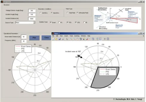
Figure 2.3 Basic flow chart of WedgeGUI ... 14

Figure 2.4 Example scenario and output of WedgeGUI: Diffracted fields vs. angle for HBC (350 , ₀45 , f 30MHz, r50m, kr31.4159). Curves belong to Exact, PTD, UTD, and PE models ... 15

Figure 2.5 Example scenario and the output of WedgeGUI: Total fields vs. angle for SBC ( 330 , ₀ 70 , f 30MHz, r50m, kr31.4159). Curves belong to Exact, PO, and PTD models. ... 16

Figure 2.6 Example scenario and the output of WedgeGUI: Diffracted fields vs. angle for HBC ( 250 , ₀ 150 , f 30MHz, r50m, kr31.4159). Curves belong to Exact, PTD, and UTD models. ... 16

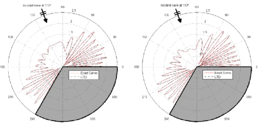
Figure 2.7 Diffracted fields vs. angle for (Left) SBC, (Right) HBC computed with Exact and UTD Models (240 ,₀ 110 , f 30MHz, r50m, kr31.4159) ... 17

Figure 2.8 Total fields vs. angle for (Left) SBC, (Right) HBC computed with Exact and UTD models ( 240 ,₀ 110 , f 30MHz, r50m, kr31.4159) ... 17

Figure 2.9 Diffraction coefficients vs. (Top) Frequency, (Bottom) Range for the plane wave illumination and SBC ( 350 , ₀ 60 , f 30MHz ) ... 18

Figure 3.1 Yee Cell ... 22

Figure 3.2 FDTD Algorithm ... 26

Figure 3.3 FDTD cell for mode ... 28

Figure 3.4 FDTD cell for mode ... 28

Figure 3.5 versus for . ... 33

Figure 3.6 versus for . ... 33

Figure 3.7 Plane wave incident on a lossy medium ... 36

Figure 3.8 Placement of PML in computational domain ... 40

Figure 3.9 FDTD simulation snapshot at ... 51

(10)

viii

Figure 3.11 FDTD simulation snapshot at ... 52

Figure 3.12 Staircase modeling missile radome ... 54

Figure 3.13 Modified Faraday loop in Dey-Mittra technique ... 54

Figure 3.14 Dey-Mittra conformal FDTD scenarios ... 55

Figure 3.15 Comparison of Dey-Mittra conformal technique (a) and Staircase approximation (b) ... 56

Figure 3.16 Multi-step FDTD-based diffraction approach: (a) The wedge scenario,(b) Infinite-plane problem, (c) Free-space scenario ... 57

Figure 3.17 Front panel of WEDGE FDTD software ... 59

Figure 3.18 Total field, Diffracted field simulation results for mode ... 60

(11)

1

1 INTRODUCTION

The phenomena of electricity and magnetism were first noticed around 600 B.C. in ancient Greece. A piece of amber rubbed with a cloth was found to attract light objects, and pieces of a magnetic core were found to attract small iron objects. They are examples of static electric and magnetic fields respectively. In 19th century, experiments made by Faraday and Ampere showed that changing magnetic field induces a changing electric field and vice-versa—the two are linked. These changing fields form electromagnetic waves which propagate in all environments. Light, microwaves, radio and TV signals are all kinds of electromagnetic waves.

When the electromagnetic wave hits a material object, time varying polarization currents occur. This time-varying polarization currents create an additional electromagnetic field which is known as scattered field and propagates into both material and its surrounding space. Scattered fields are used to identify objects at a distance. For this reason, they are important for military, biomedical, aviation and mining applications. Extensive study of scattered fields leads to many discoveries in our lives such as stealth aircrafts, cancer detection systems. Scattered field which encloses reflected field, refracted field and diffracted field, can be analyzed via using analytical techniques such as geometric optics(GO), physical theory of diffraction(PTD), physical optics(PO), exact series and exact integral, for regular geometries.

On the other hand, the exact analytical solutions for scattering, radiation and wave guiding problems are rarely available or hard to obtain, for the irregular geometries which are found in actual devices. Several numerical techniques such as FDTD, Method of Moments, Finite Element Method, are emerged to overcome these difficulties. Improvement of the computer storage and increment of processor speeds enables us to use such numerical techniques more efficiently and accurately to obtain solutions of Maxwell’s equations. Through the numerical methods, FDTD is easy to use and powerful method for obtaining numerical solutions of Maxwell’s equations in time domain as well as frequency domain via fast Fourier Transform (FFT). FDTD is based on solving differential form of

(12)

2

Maxwell’s equations via central differences. Because of being time domain method, it makes possible to observe electromagnetic wave step by step.

1.1 Outline of the Thesis

This thesis is organized as follows: In Chapter 2, we review the analytical methods used for analyzing scattered fields for non-penetrable wedge geometry [1]. After introducing the general background, we introduce WEDGE GUI which is a novel matlab based tool developed to compare different analytical results obtained from plane wave or line source illumination of wedge type obstacle.

Chapter 3 gives detailed explanation about the application of FDTD method to obtain numerical solutions of Maxwell’s equations for non-penetrable wedge type geometry. Modeling issues are also addressed in this chapter and alternative schemes are discussed to reduce numerical errors. At the end of the chapter, we introduce another novel matlab based tool WEDGE FDTD GUI which is 2D electromagnetic simulator based on FDTD method and developed to compare numerical results with analytical ones.

Although each chapter has its own concluding section, we summarize our results in chapter 4. It concludes this dissertation with a summary of the methods applied to obtain scattered fields and the future directions of our research.

(13)

3

2 ANALYTICAL METHODS

2.1 Introduction

Electromagnetic (EM) wave scattering has been substantially investigated for many decades and just reviewed with a tutorial in [1] on the canonical, two-dimensional (2D) wedge problem. Numerical difficulties of various analytical models based on complex integration as well as series summation are also discussed in details in [2]. Comparisons against numerical techniques such as the Finite-Difference Time-Domain (FDTD) method are given in [3]. In all these studies, wave pieces like reflection, refraction, and diffraction which are the components of scattering are re-visited through analytical exact as well as High Frequency Asymptotic (HFA) methods, such as Geometrical Optics (GO), Geometrical Theory of Diffraction (GTD), its uniform extension Uniform Theory of Diffraction (UTD), Physical Optics (PO), Physical Theory of Diffraction (PTD), Elementary Edge Waves (EEW), and Parabolic Equation (PE) methods [4-20].

In this section, first, the problem is posted briefly and critical wave regions are outlined. Then, mathematical equations for both plane wave and line source illuminations are presented for the sake of completeness. There are many different forms of these models, but the ones presented here are numerically the most efficient ones. Finally, the virtual tool WedgeGUI is discussed together with some examples.

The non-penetrable wedge diffraction problem is canonical and plays a fundamental role in the construction of HFA techniques as well as for the numerical tests. The exact solution to this scattering problem was first found by Sommerfeld [4] in the particular case of a half-plane. For the wedge with an arbitrary angle between its faces, the solution was obtained by Macdonald [5] and later on by Sommerfeld who developed the method of branched wave functions [6].

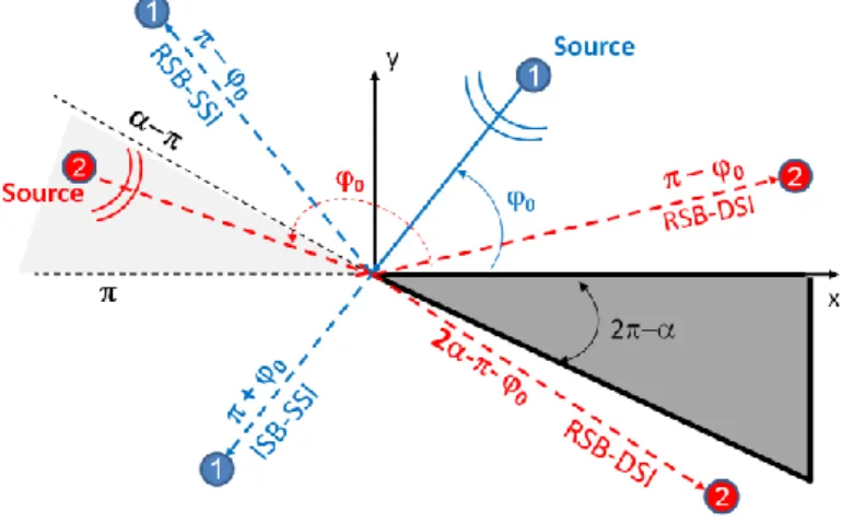
The 2D wedge scattering scenario is pictured in figure 1. The semi-infinite wedge with PEC boundaries is located in vacuum. The polar coordinates are used throughout this section. The z-axis is aligned along the edge of the wedge. The angle is measured from the top face of the wedge. The exterior angle of the wedge equals . The wedge is

(14)

4

illuminated by a Line Source (LS) at a distance from a direction. In other words, source and observation points are given by ( ) and ( ), respectively.

Figure 2.1 Geometry of the wedge scattering problem (SSI: Single Side illumination, DSI: Double Side Illumination)

The scenario for the LS-1 ( ) belongs to the Single Side Illumination (SSI) where the top face is always illuminated. In this case (i.e., for the SSI), the 2D scattering plane around the wedge may be divided into three regions in terms of critical wave phenomena occurred there. In Region–I ( ), all the field components – incident field, reflected field and diffracted field – exist. The angle is the limiting boundary of reflected fields and Region I (Reflection Shadow Boundary - RSB). In Region–II ( ) only incident and diffracted fields exist. The angle is the limiting boundary of the incident field and Region–II (Incident Shadow Boundary - ISB). In Region–III (i.e., in the shadow region, ) only diffracted fields exist.

The scenario for the LS-2 ( ) belongs to the Double Side Illumination (DSI) where both faces are always illuminated. In this case, the 2D scattering plane around the wedge may also be divided into three regions. In Region–I ( ), all the field components – incident field, reflected fields from the top face, and diffracted field – exist. The angle is the limiting boundary and called Reflection Shadow Boundary–RSB. Similarly, in Region–III ( ), all the field components – incident field, reflected fields from the bottom face, and diffracted field – exist. The angle is also a RSB. The region between these two (i.e.,

(15)

5

Region–II; ) contains no reflected fields and only incident and diffracted fields exist. In summary, both incident and diffracted fields exist everywhere, but reflected fields exist only in Region–1 and Region–3. Except the UTD formulations, the time dependence is accepted in the section. The field outside the wedge satisfies the wave equation

(2.1)

and the boundary conditions (BC)

(2.2)

and the Sommerfeld’s radiation condition at infinity:

(2.3)

In the case of EM waves, these BCs are appropriate for the PEC wedge and function us

represents the z-component of electric field intensity Ez (TM), while function uh is the

z-component of magnetic field intensity Hz (TE). In the case of acoustic waves, these

conditions refer to acoustically soft (TM > SBC) and hard (TE > HBC) wedges, respectively.

2.2 Plane Wave Illumination and HFA Models

Mathematical equations of different models are included here for both Line source (LS) and Plane Wave (PW) illuminations. The PW models presented in this section are Exact by Series Summation, PO, PTD, UTD, and PE models.

2.2.1 Exact Solution by Series Summation

The total field solutions of the Helmholtz equation with SBC and HBC for both SSI and DSI are [11]:

(16)

6 where (2.5) (2.6)

Here, and . The diffracted fields and

can be calculated by subtracting suitable components (i.e.,incident and/or reflected fields) from equation 2.4 in different regions as:

(2.7)

where, for SSI ( ) (2.8)

and for DSI ( ) (2.9)

2.2.2 The Physical Optics (PO) Solution

The diffracted fields for the PO model (i.e., the uniform part of the surface currents) are given as [11]:

For SSI ( ):

(2.10)

and, for DSI ( ):

(17)

7 where (2.12) (2.13)

Here, and . The total fields, in these cases, can be obtained via

_(2.14)

with the same GO solutions given in equations 2.8 and 2.9.

2.2.3 The PTD Solution

The PO proceeds from the hypothesis that a surface current on the illuminated side of a scattering object is determined by GO. This hypothesis is acceptable in the case of smooth objects whose radii of curvature are large compared to the wavelength; however, it neither satisfies the reciprocity principle nor the boundary conditions (BC). The PO also fails to predict depolarization of the diffracted field. The PTD improves PO by taking into account non-uniform surface currents and concentrates near edges. The PTD model is given as [11]:

(18)

8 where _(2.16) _(2.17) (2.18) (2.19) (2.20) (2.21) and (2.22) Again, the total fields, in these cases, can be obtained via

(2.23)

(19)

9

2.2.4 The UTD Solution

The UTD diffracted fields are in the form of

(2.24)

where and the time dependence is . According to the UTD, the diffraction coefficients for SBC and HBCs with line source as follows [13]

(2.25) (2.26)

where , and is the Fresnel function given as

(2.27) and are determined as in [9]:

(2.28)

Here, are the integers which most nearly satisfy the last equation given in equation 2.28. Note that the cotangent functions in equations 2.25 and 2.26 become singular at the ISB and RSB and are replaces as [13]:

(20)

10

for small . This term is finite but discontinuous at the ISB and RSB and compensates the discontinuities of the incident or reflected fields at these boundaries. The UTD based total fields are then obtained by adding the GO fields appropriately:

Again, the total fields, in these cases, can be obtained via

(2.30)

with the GO solutions given as for SSI ( ) (2.31)

and for DSI ( )

(2.32) Note that, the UTD formulas are exactly the same for the line source excitation, except in is replaces with .

2.2.5 The Parabolic Equation (PE) Solution

As shown in [10] the method of Parabolic Equation (PE) provides a correct first-order approximation to the diffracted field in the case when and .

(2.33) where (2.34) (2.35) with and

. Again, the total fields, in these cases, can be obtained via

(21)

11

(2.36) with the same GO solutions given in equations 2.8 and 2.9.

2.3 HFA Models under Line Source Excitations

Mathematical equations of the models Exact by Series, Exact by Integral, the UTD, and PE, Line source (LS) illumination are presented in this section. Note that, numerical results of these models match with the PW models given in the previous section when the source-to-tip distance is large as compared with the wavelength.

2.3.1 Exact Solution by Series Summations

The total field solutions of the Helmholtz equation with SBC and HBC for both SSI and DSI are [11]: (2.37) (2.38)

with the same given in equation 2.6. Normalized diffracted fields can be obtained by subtracting GO fields

(2.39) The GO field that under LS excitation is given as follows:

(22)

12 For SSI: (2.40) For DSI: (2.41)

where and for SBC and HBC respectively, and

(2.42)

(2.43)

(2.44)

2.3.2 Exact Solution by Integral

Solutions for the line source illumination are also well known and presented by Bowman and Senior in Handbook [8] as

(2.45) (2.46) where (2.47) and . In this case, total fields are obtained by

(23)

13

adding the GO fields. Again, the total fields, in these cases, can be obtained via

(2.48) with the same GO solutions given in equations 2.8 and 2.9.

2.3.3 The Parabolic Equation (PE) Solution

The PE solution under a line source illumination when and can be listed as follows [10]: (2.49) where (2.50) (2.51)

with , and . Again, the total fields, in these cases, can be obtained via (2.52)

with the same GO solutions are given in equations 2.8 and 2.9.

2.4 The WedgeGUI Virtual Tool and Some Examples

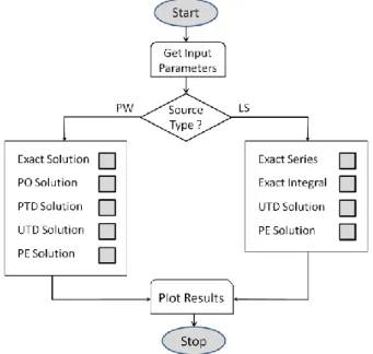
The Matlab-based simulation package WedgeGUI with the front panel displayed in figure 2.2, is prepared for the investigation of wedge diffraction in 2D with various HFA models. The panel is divided into three parts. The top block is reserved for the structure. The wedge figure is shown on the top right. The wedge exterior angle incident distance and angle are supplied on the top left. The user also selects either of the Soft and Hard boundary conditions and total and diffracted fields in this block. A pop-up menu allows the user to choose the type of the source: Plane wave excitation or cylindrical wave excitation. For

(24)

14

each source type the methods used in simulations are given with tick boxes. Multiple selection is possible. The flow chart of the virtual tool is given in figure 2. 3.

Figure 2.2 The front panel of the EM virtual tool WedgeGUI

(25)

15

The area below the structure block is divided into two parts. On the left, the results are presented in terms of polar plots (i.e., fields vs. angle), on the right in terms of Cartesian plots (i.e., field vs. radial range or field vs. frequency). For the polar plots on the left block, one needs to specify frequency and radial distance from the tip. The rest is handled automatically once the Plot button is pressed and fields are calculated at N observation points equidistant from the tip located apart. The progress bar on the bottom-left shows the status of the calculations. Figures 2.4-2.6 show example scenarios and simulation results.

The user may edit/modify the plot in another figure window. This is possible by clicking on the polar plot. Similarly, one can plot field vs. range or field vs. frequency on the right block. Clear button clears the plot for the next simulation and Save Data button records the data in a text file with the name given by the user. Table 1 lists a sample recorded data (partially) which belongs to the simulations presented in figure 2.6. Data recording is important because WedgeGUI do not run simulations for both SBC and HBC, or both total and diffracted fields at the same time. One needs to run WedgeGUI twice for the examples presented in figures 2.7-2.9.

Figure 2.4 Example scenario and output of WedgeGUI: Diffracted fields vs. angle for HBC ( 350 , 0 45

(26)

16

Figure 2.5 Example scenario and the output of WedgeGUI: Total fields vs. angle for SBC ( 330 , 0 70

  , f 30MHz, r50m, kr31.4159). Curves belong to Exact, PO, and PTD models.

Figure 2.6 Example scenario and the output of WedgeGUI: Diffracted fields vs. angle for HBC ( 250 , 0 150

(27)

17

Table 1. Sample recorded data for angle vs. diffracted fields.

Figure 2.7 Diffracted fields vs. angle for (Left) SBC, (Right) HBC computed with Exact and UTD Models (

240

  ,₀ 110 , f 30MHz, r50m, kr31.4159)

Figure 2.8 Total fields vs. angle for (Left) SBC, (Right) HBC computed with Exact and UTD models (

240

(28)

18

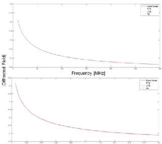
Figure 2.9 Diffraction coefficients vs. (Top) Frequency, (Bottom) Range for the plane wave illumination and SBC (350 , ₀ 60 , f 30MHz )

2.5 Conclusions

A MatLab-based virtual diffraction tool, WedgeGUI, is introduced. The WedgeGUI presents results of electromagnetic wave scattering from a wedge shaped object with Perfectly Electrical Conductor (PEC) boundaries under different structural as well as operational parameters. Various models under both line source and plane wave illuminations are included. Comparisons among Uniform Theory of Diffraction (UTD), Physical Optics (PO), Physical Theory of Diffraction (PTD), Parabolic Equation (PE) models through many scenarios and illustrations are possible. The WedgeGUI virtual tool can be used in many graduate and PhD level courses such as Advanced Electromagnetic Theory, High Frequency Asymptotic Methods in Electromagnetics, Diffraction Theory, etc.

(29)

19

3 FINITE DIFFERENCE TIME DOMAIN (FDTD) METHOD

3.1 Introduction

FDTD method is introduced by Yee in 1966 [21] is arguably the simplest of numerical methods used to solve electromagnetic problems. It is based on simple formulations which don’t require complex asymptotic or Green’s functions. Yee’s idea was to divide simulation space into cells to form a grid and solve differential form of the Maxwell’s equations around these cells by using second-order central differences. Although it is time domain based method, it can provide frequency domain responses via Fourier transform. FDTD has been used to solve various types of problems arises in our lives including scattering, radar cross section, cancer detection, cell phone radiation over human head and geological applications.

Since FDTD is based on discretizing time and simulation space, it is useful to explain numerical derivatives. Taylor series expansion of the multivariable function around the specified time can be written as;

(3.1)

If the function is sampled in time with intervals we can write equation 3.1 as follows

(3.2)

After rearranging terms we obtain: (3.3)

In a similar manner, the same expansion can be repeated for finding space derivative of the function. The terms in the Taylor series extends to infinity and due to the discrete nature of the computers, this expansion should be truncated after desired accuracy is obtained. As it

(30)

20

is seen by the equation (3.3) the other terms multiplied with the orders of . According to truncation of terms there are several numerical derivative approximations. If we omit the terms which multiplied with the orders of in equation 3.3, we obtain:

(3.4)

This approximation is called first-order forward difference approximation of the derivative of the function . The term ―first-order‖ comes from the fact that we omitted the terms multiplied with the orders of starting from the first order in the equation (3.3). The term ―forward‖ comes from the fact that, one forward time is used to evaluate derivative.

In kind, expansion of around the point gives (3.5)

Leaving the first order derivative alone we have (3.6)

Neglecting the terms multiplied with the powers of t, we obtain the first-order backward approximation of the derivative of the function .

(3.7)

The third way of obtaining a formula for an approximation of the derivative is obtained by averaging the forward and backward difference formulas such that

(3.8)

(31)

21 (3.9)

In this case there is no term multiplied with first order of . Neglecting the terms multiplied with the powers of gives second-order centered difference approximation.

(3.10)

The error introduced by using this approximation is less than the first-order forward or backward approximations. For example, if the time step is reduced to half of its value the error reduced by a factor of four.

3.2 3D FDTD Algorithm

Yee’s algorithm approximates the derivatives in the differential form of Maxwell’s equations shown in equations 3.11 – 3.14 with second-order centered differences.

(3.11) (3.12) (3.13) (3.14) where is .

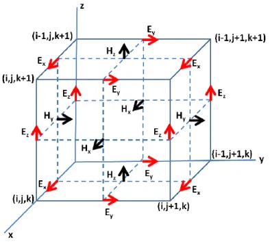
The spatial positions of the field components have specific arrangement in the Yee cell as shown in figure 3.1. In this arrangement electric fields are placed at the centers of the edges of Yee cell and magnetic fields are placed at the center of the faces of the Yee cell. In other words, magnetic field components are surrounded by four electric field components and electric field components are surrounded by four magnetic field components. Instead, one can rearrange Yee cell so that location of the magnetic and electric field components are interchanged. But this arrangement has advantage because of the fact that boundary conditions imposed on electric field are more commonly encountered than those for magnetic field so placing the mesh boundaries so that they pass

(32)

22

through electric field vectors [22]. In addition to spatial arrangement, Yee assumed that the magnetic field components are calculated at half time steps slightly after electric field components. Therefore super script n+1/2 is used for magnetic fields to emphasize that they are calculated slightly after electric fields.

Figure 3.1 Yee Cell

Since we know the spatial locations of the field components, we are ready to discrete Maxwell’s equations. We first start with writing open form of curl operator in equation 3.13. (3.15)

Here we omitted the by omitting magnetic current density M and electric current density J. Writing and equating with the left side of the equation 3.15 yields three coupled scalar equations:

(33)

23 (3.16) (3.17) (3.18)

Repeating the same process for equation 3.14 we obtain:

(3.19)

In a similar manner, Writing and equating with the left side of the equation 3.19 yields three coupled scalar equations:

(3.20) (3.21) (3.22)

Referring to figure 3.1, we can approximate the derivatives of the equations 3.16 – 3.22 via second-order centered differences. Applying the second-order centered difference approximation to the time and space derivatives in equation 3.16 yields:

(34)

24 (3.23)

Rearranging terms in equation 3.23, we obtain: (3.24)

In equation 3.24 we have used compact form field components i.e.

. Here, superscript n is used for time step and subscript i, j, k is used for spatial location. The remaining components are presented in the equations 3.25 – 3.30. (3.25) (3.26)

(35)

25 (3.27) (3.28) (3.29)

Time step is explicit in FDTD algorithm such that magnetic fields are calculated before/after the electric fields. So we can disregard half-time step superscript in the equations 3.24-3.29. On the other hand, spatial steps are implicit and we cannot use double

(36)

26

numbers as an array index in high-level programming languages. Hence, we can apply the following rules to solve half-step problem:

When it comes to calculating E values of i, j, k indexes then the indexes of the necessary H value follow this rule:

 When the H index has a +1/2 assume its value 0

 When the H index has a -1/2 assume its value -1

When it comes to calculating H values of i, j, k indexes then the indexes of the necessary E value follow this rule:

 When the H index has a -1/2 assume its value 0

 When the H index has a +1/2 assume its value +1

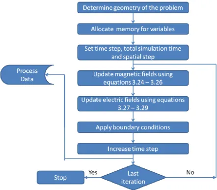
The complete FDTD algorithm is shown at figure 3.2.

Figure 3.2 FDTD Algorithm

In this algorithm, selection of time step and spatial step requires specific attention as will be explained later.

(37)

27

3.3 Reduction to 2D

and Modes

When both the structure being modeled and the excitation do not change with respect to specific direction, then the derivatives in Maxwell’s curl equations (3.15 and 3.19) with respect to that direction vanish. For example, if the problem is z dimension independent we have: (3.30) (3.31)

We can group equations 3.30 and 3.31 into two uncoupled sets called transverse magnetic ( and transverse electric modes as follows:

Mode (3.32) Mode (3.33)

(38)

28

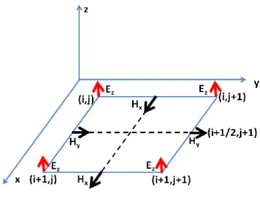
As it is seen by equations 3.32 and 3.33 and modes don’t contain common field components and they are identified as which have a magnetic or electric field component in the axial (i.e. z) direction. Although the spatial locations of the field components are shown at figure 3.1, we present 2D slices obtained from figure 3.1 in figures 3.3 and 3.4 for clarity.

Figure 3.3 FDTD cell for mode

(39)

29

FDTD update equations for both and modes can be obtained by applying central difference approximation to the partial derivatives in the equations 3.32 and 3.33. For the sake of completeness we present them as follows:

Mode (3.34) (3.35) (3.36) Mode (3.37) (3.38) (3.39)

(40)

30

Most two-dimensional problems can be decomposed into and modes and can be solved separately because of the fact that they are uncoupled. The solution for the main problem is then obtained by summing the solutions of and modes.

3.4 Numerical Dispersion

Dispersion relation gives the relationship between wavelength and frequency. Dispersion occurs when the waves of different frequencies have different propagation velocities. For electromagnetic waves in vacuum, the frequency is proportional with wavelength and dispersion relation is given as:

(3.40)

In this chapter will try to find a dispersion relation for FDTD algorithm. For this purpose, we will analyze 2D FDTD algorithm for simplicity but the results can be extended to 3D FDTD algorithm easily. It is obvious that the following traveling-wave equations are the solutions of mode equations (3.37-3.39):

(3.41)

(3.42)

_(3.43)

where are the components of the numerical wavevector.

Using equations 3.41-3.43 in equation 3.37, we obtain the following equation. (3.44)

Dividing both sides of the equation by

(41)

31 (3.45)

Additional simplification can be achieved by using Euler’s formula:

(3.46)

In kind, the following equations can be derived for and

(3.47) (3.48)

Upon substituting and into equation 3.48, we obtain

(3.49)

where _{is the phase velocity.}

Equation 3.49 is the general numerical dispersion relation for the mode. Assuming and writing and , this equation can be written as

(42)

32 (3.50)

Dividing both sides of equation 3.50 by leads the following equation

(3.51)

where is the speed of light, is numerical phase velocity and is the propagation direction with respect to x axes. It is obvious that both and affects numerical dispersion and should be carefully selected. Setting and selecting in equation 3.51 leads to

(3.52)

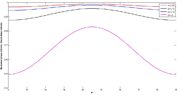
That is numerical wave propagates exactly with the speed of light. Therefore, we can recover the ideal dispersion relation by selecting appropriate values. The dependence of on propagation angle is called grid anisotropy. We demonstrate how the numerical phase velocity changes with propagation angle in figure 3.5 for and in figure 3.6 for

(43)

33

Figure 3.5 versus for .

Figure 3.6 versus for .

It is evident that increasing sampling resolution decreases numerical dispersion error. What’s more, we cannot totally eliminate numerical dispersion error because we are restricted to work with finite grid cells. For this reason, numerical dispersion error is inherited to FDTD algorithm, but this error is very small even for resolution.

(44)

34

3.5 Stability

In this section, we analyze how selection of time step affects stability of the FDTD algorithm. For this purpose, we will use complex-frequency analysis which allows for the possibility of a complex-valued numerical angular frequency, [23]. We start first by modifying the angular frequency term in equation 3.43 as follows

(3.53)

If the term in equation 3.53 is positive, we have exponentially decreasing wave amplitude. On the other hand, if is negative, we have exponentially increasing wave amplitude. In section 3.4 we have derived an expression of the numerical angular frequency which is written again for clarity

(3.54)

In this equation, if the term inside the arcsin function has value between 0 and 1, we obtain real numerical angular frequency. We can also observe from the equation 3.54 that the upper bound of the expression in square root is

(3.55)

Therefore, we can write

(45)

35

To ensure stability we should select the time step as

(3.57)

When , equation 3.57 becomes

(3.58)

This expression tells us that, the electromagnetic wave should travel at most one cell diagonally in one time step.

In a similar manner for 3D FDTD, the time step t should be selected as

(3.59)

3.6 Perfectly Matched Layer Boundary Conditions

Scattering and radiation problems require the simulation space which extends infinity. Due to the finite nature of computers we cannot use infinite number of cells. Even if we are interested in near fields, we need to enlarge total simulation space to prevent reflections from the boundaries. However, increasing total simulation space increases the computational burden excessively. So far, several methods proposed to overcome this difficulty [23]. These methods split into two groups, one called absorbing boundary conditions (ABC), the other called radiation boundary conditions (RBC). RBCs require the storage of field components more than one time step back depending on the order of accuracy. Hence, they can cause out of memory errors for large problems. Also since they are a function of incident angle, they can give spurious reflections for grazing angles. On the other hand, ABCs don’t require the storage of field components more than one time step back, and give more accurate results with compare to RBCs. Among ABCs, the perfectly matched layer (PML) boundaries are very popular and easy to implement. PML is a finite-thickness special lossy medium which is placed at the terminals of the computational space to create perfectly matching condition for all angles and frequencies.

(46)

36

Because of being frequency and angle independent, they are used in scattering and radiation problems frequently. There are several types of PMLs found in literature such as uniaxial PML (UPML), convolutional PML (CPML), split-field PML (SPML), and the detailed comparison of their properties can be found in [24]. In this dissertation we preferred to use UPML so this type of PML will be explained. We will start by reviewing electromagnetic wave behavior at the boundary of two dissimilar media to explain the underlying theory of PMLs.

3.6.1 Plane Wave Incident on a Lossy Medium

Considering a polarized field shown in figure 3.7 where the incident electric field phasor is given by

(3.60)

(47)

37 The incident magnetic field is then calculated from

(3.61)

Assuming a presence of reflected wave and knowing that the angle of incidence equals to angle of reflection, we have

(3.62)

where

is the reflection coefficient. Notice that the change of sign in equation 3.62 due to the reflection. Then we can write the total electric fields in region 1 as

(3.63) In kind, using equation 3.61 we can write the total magnetic fields in region 1 as

(3.64)

Now we can consider the electromagnetic fields in region 2 which is lossy medium characterized with the parameters and . For this reason we can write the time harmonic Maxwell’s equations for general lossy media as follows

(3.65) (3.66)

(48)

38

Therefore the transmitted electric field in Region 2 can be written as

_(3.67)

where is the transmission coefficient. The magnetic fields in Region 2 are calculated using equation 3.65 as follows

(3.68) where , (3.69)

is the propagation constant.

Owing to the boundary condition that is the continuity of the tangential fields at the interface (x=0), the propagation in the y direction must be same in both media yields

_(3.70)

Thus we can say that

(3.71)

(49)

39

(3.72)

Equating y component of the magnetic fields at x=0 we obtain

_(3.73)

In this case, we can say that

(3.74)

The reflection and transmission coefficients are given by [25]

(3.75) and (3.76)

Reflection coefficient will be zero only if the terms in the numerator of equation 3.75 cancel. Also it is seen that, for an arbitrary incident angle we have complex and non-zero reflection number. Assuming the incident wave , the expression in equation 3.75 reduces to

(3.77)

(50)

40 and (3.78)

Selecting yields that , perfectly matching wave transmission at the boundary. But, for oblique incidence, the numerator of the term in equation 3.75 cannot be zero and there will always be reflection from region 2.

3.6.2 Uniaxial Perfectly Matched Layer (PML)

Among the different versions of the PML, the uniaxial perfectly matched layer (PML) is arguably simplest to understand and has been broadly used in the FDTD simulations. In UPML, lossy layer is described as an artificial anisotropic uniaxial absorbing material which is composed of both electric and magnetic permittivity tensors. The main advantage of the UPML is that we don’t require changing our code in both computational region and PML region. Therefore, the FDTD algorithm remains same in both domains. The placement of the PML in computational space is shown in figure 3.8.

(51)

41

We can assume that the region 2 ( ) in figure 3.7, as an anisotropic uniaxial medium which is rotationally symmetric around the x axis and having the electrical permittivity and magnetic permeability tensors:

(3.79)

Also we assume that a TE polarized time-harmonic wave

propagates through region 2. As we did in previous chapter for mode, we can write total electric and magnetic fields in the region 1 as

_(3.80) (3.81)

Electromagnetic waves in region 2 satisfy the Maxwell’s equations in a general anisotropic medium which can be expressed in phasor form as:

(3.82) (3.83) where

(3.84)

is the wavevector in region 2. Combining equations 3.82 and 3.83 leads to wave equation given as:

_(3.85) which can also be written in matrix form as:

(52)

42 (3.86)

The solutions of the determinant of the matrix in equation 3.86 give the relationship between the wave numbers that is called dispersion relation as we mentioned in section 3.4. There are two solutions of equation 3.86 which are called TE mode ( and TM mode ( . We assume only TE mode solution which is obtained at setting

in equation 3.86 as

(3.87)

The wave transmitted in region 2 can be expressed in a manner similar to equation 3.68 as (3.88)

Owing to the boundary condition that is the continuity of the tangential fields at the interface (x=0), the propagation in the y direction must be same in both media yields

(3.89) and (3.90)

(53)

43

Since for all incident angles, we can put this equality into equation 3.87 to obtain the value of as

(3.91)

What’s more, we can find the reflection coefficent from 3.90 as (3.92)

To achive perfectly matching at the boundary, we need to have which means that the nominator of equation 3.92 should be zero. From inspection, selecting , , and _yields

(3.93)

Putting equation 3.93 into equation 3.92 we have for all incidence angles and . Thus the incident wave penetrates into region 2 without any reflection. Since we have found in equation 3.93, we can put this into equation 3.88 to analyze the wave behavior in region 2 as (3.94) Selecting yields (3.95)

It is obvious that the magnetic field attenuates exponentially through the propagation in region 2 for all incident wave angles and . In a similar manner the electric field also undergoes an exponential decay through the propagation in region 2. The same analysis can be performed for TM mode. But in this case we need to replace and

(54)

44

and set for reflectionless propagation. In sum, we can write the permittivity and permeability tensors to have at the boundary as

(3.96)

UPML extension for 3D case can be obtained easily by considering 3D case is a composition of individual lossy layers. That is, we need to place individual lossy layers at the front ends of the x, y and z dimensions of computational space. Then, the electric permittivity and magnetic permeability tensors will be in the form as

(3.97) where (3.98) Here the parameters are introduced for allowing non-unity real part. To use this tensor in FDTD algorithm we need to set non-zero conductivity at appropriate boundaries as demonstrated in figure 3.8. For example at and we need to set .

3.6.3 UPML Algorithm

In this section, we will derive 3D numerical algorithm for implementing uniaxial perfectly matched layer medium formulated previously. Maxwell’s equations for general anisotropic media are given in phasor form by equations 3.82 and 3.83, repeated below for convenience:

(55)

45

(3.100) Writing the curl operator of equation 3.100 in matrix form and using the tensor which is introduced in equation 3.97 leads to

(3.101)

Then we have from the first row of the matrix equation:

(3.102)

At this point, it is instructive to give some properties of the phasor to time domain transformations.

(3.103)

(3.104)

Converting equation 3.102 directly from phasor domain to time domain requires integration because of the term in the denominator and integration is very computationally expensive process especially for large problems. To overcome this difficulty, we can use interim variable which is not physical and formed as

(3.105)

(56)

46 (3.106)

This leaves us to three equations which can be transformed into time domain easily by using equation 3.103. Moreover, since FDTD algorithm is based on discretizing partial derivatives in Maxwell’s equations via centered difference approximation, we can apply the same approximation to discretize the resulting interim fields. This provides us to conserve our codes in both computational region and PML region with the expense of doubling field components which is explained soon. But anyway, this is computationally less expensive than calculating integrals. Considering the first equation in 3.106, we have

(3.107)

Applying equation 3.103 to 3.107 yields (3.108)

The components of auxiliary fields is assumed to be same location as the components of electric fields as shown in figure 3.1, therefore applying centered difference approximation to equation 3.108 gives (3.109)

(57)

47

The other auxiliary field components can be derived in a similar manner, they are given here for the sake of completeness

(3.110) (3.111)

Now we need to convert interim fields back to electric field components. This is also can be accomplished easily as shown for the x component:

(3.112)

Applying equation 3.103 to equation 3.112 leads

(3.113)

Discretization of equation 3.113 yields update equation for the x component of the electric field:

(58)

48 (3.114)

The same analysis can be repeated for the remaining components of electric fields, and given as follows (3.115) (3.116)

Thus far, we are concerned with the electric field components. The magnetic fields can be calculated in a similar manner by writing the curl operator of equation 3.99 in matrix form as follows (3.117)

In the same way for electric fields, we introduce auxiliary field B to get rid of integrals as shown below:

_(3.118)

(59)

49 (3.119)

Considering the first equation in 3.119, we obtain the following equation (3.120)

Applying centered difference approximation to the partial derivatives of equation 3.120 yields updating equation for the interim field component whose spatial location is the same as and shown in the figure 3.1.

(3.121)

Doing same analysis as in equation 3.120 for remaining interim fields we obtain (3.122) (3.123)

(60)

50

The relationship between the interim fields and magnetic fields is similar to that of interim field and and can be given as

(3.124)

Applying inverse transformation to equation 3.124 yields

(3.125)

Equation 3.125 can be discretized as (3.126)

The remaining magnetic field components can be obtained in a similar manner as follows (3.127)

(61)

51 (3.128)

The implementation of the UPML algorithm requires two step for updating individual electric and magnetic fields. That is, we first need to solve interim fields and then calculate electric and magnetic fields from the interim fields as shown in the related equations. Also we need to store one time step previous values of the interim fields because the magnetic and electric field updates require the values of interim fields at time or . Although, we explain the algorithm of 3D UPML, reduction to 2D case is straightforward and explained briefly in section 3.3. We have taken three snapshots at different time steps to demonstrate the PML boundary condition in 2D mode as shown in figures 3.9, 3.10 and 3.11. We have injected Gaussian source at the center of the simulation space.

(62)

52

Figure 3.10 FDTD simulation snapshot at

Figure 3.11 FDTD simulation snapshot at

Source codes for this simulation can be found in Appendix 1. An ideal PML is reflectionless, if the parameters of the PML are selected properly as described previously. However, because of the numerical approximations, the PML in FDTD simulations cannot absorb the power penetrating into PML regions properly and consequently can lead to significant spurious reflections. To overcome this problem, we need to use multilayer PML instead [26]. The term multilayer means that the conductivity profile of the lossy layer changes with spatial increment. There are several methods to create such a multilayer PML but arguably most effective one is polynomial grading whose formulation is given as