Study of the underlying event in top quark pair production in pp collisions at 13 TeV

CERN-EP-2018-177 2019/02/11

CMS-TOP-17-015

Study of the underlying event in top quark pair production

in pp collisions at 13 TeV

The CMS Collaboration

∗

Abstract

Measurements of normalized differential cross sections as functions of the multiplic-ity and kinematic variables of charged-particle tracks from the underlying event in top quark and antiquark pair production are presented. The measurements are per-formed in proton-proton collisions at a center-of-mass energy of 13 TeV, and are based on data collected by the CMS experiment at the LHC in 2016 corresponding to an in-tegrated luminosity of 35.9 fb−1. Events containing one electron, one muon, and two jets from the hadronization and fragmentation of b quarks are used. These measure-ments characterize, for the first time, properties of the underlying event in top quark pair production and show no deviation from the universality hypothesis at energy scales typically above twice the top quark mass.

Published in the European Physical Journal C as doi:10.1140/epjc/s10052-019-6620-z.

c

2019 CERN for the benefit of the CMS Collaboration. CC-BY-4.0 license ∗_{See Appendix B for the list of collaboration members}

1

Introduction

At the LHC, top quark and antiquark pairs (tt) are dominantly produced in the scattering of the proton constituents via quantum chromodynamics (QCD) at an energy scale (Q) of about two times the t quark mass (mt). The properties of the t quark can be studied directly from

its decay products, as it decays before hadronizing. Mediated by the electroweak interaction, the t quark decay yields a W boson and a quark, the latter carrying the QCD color charge of the mother particle. Given the large branching fraction for the decay into a bottom quark, B(t_→Wb) =0.957_±0.034 [1], in this analysis we assume that each t or t quark yields a corre-sponding bottom (b) or antibottom (b) quark in its decay. Other quarks may also be produced, in a color-singlet state, if a W → qq0 decay occurs. Being colored, these quarks will fragment and hadronize giving rise to an experimental signature with jets. Thus, when performing pre-cision measurements of t quark properties at hadron colliders, an accurate description of the fragmentation and hadronization of the quarks from the hard scatter process as well as of the “underlying event” (UE), defined below, is essential. First studies of the fragmentation and hadronization of the b quarks in tt events have been reported in Ref. [2, 3]. In this paper, we present the first measurement of the properties of the UE in tt events at a scale Q_≥2mt.

The UE is defined as any hadronic activity that cannot be attributed to the particles stemming from the hard scatter, and in this case from tt decays. Because of energy-momentum conser-vation, the UE constitutes the recoil against the tt system. In this study, the hadronization products of initial- and final-state radiation (ISR and FSR) that cannot be associated to the par-ticles from the tt decays are probed as part of the UE, even if they can be partially modeled by perturbative QCD. The main contribution to the UE comes from the color exchanges between the beam particles and is modeled in terms of multiparton interactions (MPI), color reconnec-tion (CR), and beam-beam remnants (BBR), whose model parameters can be tuned to minimum bias and Drell–Yan (DY) data.

The study of the UE in tt events provides a direct test of its universality at higher energy scales than those probed in minimum bias or DY events. This is relevant as a direct probe of CR, which is needed to confine the initial QCD color charge of the t quark into color-neutral states. The CR mainly occurs between one of the products of the fragmentation of the b quark from the t quark decay and the proton remnants. This is expected to induce an ambiguity in the origin of some of the final states present in a bottom quark jet [4–6]. The impact of these ambiguities in the measurement of t quark properties is evaluated through phenomenological models that need to be tuned to the data. Recent examples of the impact that different model parameters have on mtcan be found in Ref. [7, 8].

The analysis is performed using final states where both of the W bosons decay to leptons, yield-ing one electron and one muon with opposite charge sign, and the correspondyield-ing neutrinos. In addition, two b jets are required in the selection, as expected from the tt_{→ (}eνb)(µνb)decay. This final state is chosen because of its expected high purity and because the products of the hard process can be distinguished with high efficiency and small contamination from objects not associated with t quark decays, e.g., jets from ISR.

After discussing the experimental setup in Section 2, and the signal and background modeling in Section 3, we present the strategy employed to select the events in Section 4 and to measure the UE contribution in each selected event in Section 5. The measurements are corrected to a particle-level definition using the method described in Section 6 and the associated systematic uncertainties are discussed in Section 7. Finally, in Section 8, the results are discussed and compared to predictions from different Monte Carlo (MC) simulations. The measurements are summarized in Section 9.

2

The CMS detector

The central feature of the CMS apparatus is a superconducting solenoid of 6 m internal diame-ter, providing a magnetic field of 3.8 T parallel to the beam direction.

Within the solenoid volume are a silicon pixel and strip tracker, a lead tungstate crystal elec-tromagnetic calorimeter (ECAL), and a brass and scintillator hadron calorimeter (HCAL), each composed of a barrel and two endcap sections. A preshower detector, consisting of two planes of silicon sensors interleaved with about three radiation lengths of lead, is located in front of the endcap regions of the ECAL. Hadron forward calorimeters, using steel as an absorber and quartz fibers as the sensitive material, extend the pseudorapidity coverage provided by the barrel and endcap detectors from|η| =3.0 to 5.2. Muons are detected in the window|η| <2.4 in gas-ionization detectors embedded in the steel flux-return yoke outside the solenoid. Charged-particle trajectories with_|η| <2.5 are measured by the tracker system. The particle-flow algorithm [9] is used to reconstruct and identify individual particles in an event, with an optimized combination of information from the various elements of the CMS detector. The energy of the photons is directly obtained from the ECAL measurement, corrected for zero-suppression effects. The energy of the electrons is determined from a combination of the elec-tron momentum at the primary interaction vertex as determined by the tracker, the energy of the corresponding ECAL cluster, and the energy sum of all bremsstrahlung photons spatially compatible with originating from the electron track. The energy of the muons is obtained from the curvature of the corresponding track. The energy of charged hadrons is determined from a combination of their momentum measured in the tracker and the matching ECAL and HCAL energy deposits, corrected for zero-suppression effects and for the response function of the calorimeters to hadronic showers. Finally, the energy of neutral hadrons is obtained from the corresponding corrected ECAL and HCAL energies.

Events of interest are selected using a two-tiered trigger system [10]. The first level, composed of custom hardware processors, uses information from the calorimeters and muon detectors to select events at a rate of around 100 kHz within a time interval of less than 4 µs. The second level, known as the high-level trigger, consists of a farm of processors running a version of the full event reconstruction software optimized for fast processing, and reduces the event rate to around 1 kHz before data storage.

A more detailed description of the CMS detector, together with a definition of the coordinate system used and the relevant kinematic variables, can be found in Ref. [11].

3

Signal and background modeling

This analysis is based on proton-proton (pp) collision data at a center-of-mass energy √s = 13 TeV, collected by the CMS detector in 2016 and corresponds to an integrated luminosity of 35.9 fb−1[12].

The tt process is simulated with the POWHEG (v2) generator in the heavy quark production (hvq) mode [13–15]. The NNPDF3.0 next-to-leading-order (NLO) parton distribution functions (PDFs) with the strong coupling parameter αS = 0.118 at the Z boson mass scale (MZ) [16] are

utilized in the matrix-element (ME) calculation. The renormalization and factorization scales, µRand µF, are set to mT =

√

m2_t +p2_T, where mt =172.5 GeV and pTis the transverse

momen-tum in the tt rest frame. Parton showering is simulated using PYTHIA8 (v8.219) [17] and the CUETP8M2T4 UE tune [18]. The CUETP8M2T4 tune is based on the CUETP8M1 tune [19] but uses a lower value of αISR

description of jet multiplicities in tt events at√s = 8 TeV [20]. The leading-order (LO) version of the same NNPDF3.0 is used in the PS and MPI simulation in the CUETP8M2T4 tune. The cross section used for the tt simulation is 832+₋20₂₉ (scale)_±35(PDF+αS)pb, computed at the

next-to-next-to-leading-order (NNLO) plus next-to-next-to-leading-logarithmic accuracy [21]. Throughout this paper, data are compared to the predictions of different generator settings for the tt process. Table 1 summarizes the main characteristics of the setups and abbreviations used in the paper. Among other UE properties, CR and MPI are modeled differently in the alterna-tive setups considered, hence the interest in comparing them to the data. Three different signal ME generators are used: POWHEG, MADGRAPH5 aMC@NLO (v2.2.2) with the FxFx merging scheme [22, 23] for jets from the ME calculations and PS, andSHERPA(v2.2.4) [24]. The latter is used in combination with OPENLOOPS(v1.3.1) [25], and with the CS parton shower based on the Catani–Seymour dipole subtraction scheme [26]. In addition, two differentHERWIGPS ver-sions are used and interfaced withPOWHEG: HERWIG++ [27] with the EE5C UE tune [28] and the CTEQ6 (L1) [29] PDF set, andHERWIG7 [27, 30] with its default tune and the MMHT2014 (LO) [31] PDF set.

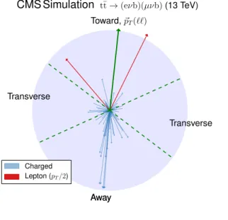
Table 1: MC simulation settings used for the comparisons with the differential cross section measurements of the UE. The table lists the main characteristics and values used for the most relevant parameters of the generators. The row labeled “Setup designation” shows the defini-tions of the abbreviadefini-tions used throughout this paper.

Event generator POWHEG(v2) MADGRAPH5 aMC@NLO(v2.2.2) SHERPA(v2.2.4) Matrix element characteristics

Mode hvq FxFx Merging OPENLOOPS

Scales (µR, µF) mT ∑t,tmT/2 METS + QCD

αS(MZ) 0.118 0.118 0.118

PDF NNPDF3.0 NLO NNPDF3.0 NLO NNPDF3.0 NNLO

Accuracy tt [NLO] tt + 0,1,2 jets [NLO] tt [NLO]

1 jet [LO] 3 jets [LO] Parton shower

Setup designation PW+PY8 MG5 aMC SHERPA

PS PYTHIA(v8.219) CS

Tune CUETP8M2T4 default

PDF NNPDF2.3 LO NNPDF3.0 NNLO

(αISR_S (MZ), αFSRS (MZ)) (0.1108, 0.1365) (0.118, 0.118)

ME Corrections on —

Setup designation PW+HW++ PW+HW7

PS HERWIG++ HERWIG7

Tune EE5C Default

PDF CTEQ6 (L1) MMHT2014 LO

(αISR_S (MZ), αFSRS (MZ)) (0.1262, 0.1262) (0.1262, 0.1262)

ME Corrections off on

Additional variations of the PW+PY8 sample are used to illustrate the sensitivity of the mea-surements to different parameters of the UE model. A supplementary table, presented in the appendix, details the parameters that have been changed with respect to the CUETP8M2T4 tune in these additional variations. The variations include extreme models that highlight sepa-rately the contributions of MPI and CR to the UE, fine-grained variations of different CR mod-els [5, 32], an alternative MPI model based on the “Rope hadronization” framework describing Lund color strings overlapping in the same area [33, 34], variations of the choice of αS(MZ)in

accord-ing to their uncertainties.

Background processes are simulated with several generators. The WZ, W+jets, and ZZ_→2`2q (where ` denotes any of the charged leptons e/µ/τ) processes are simulated at NLO, using MADGRAPH5 aMC@NLOwith the FxFx merging. Drell–Yan production, with dilepton invari-ant mass, m(``), greater than 50 GeV, is simulated at LO with MADGRAPH5 aMC@NLO us-ing the so-called MLM matchus-ing scheme [35] for jet mergus-ing. The POWHEG (v2) program is furthermore used to simulate the WW, and ZZ → 2`2ν processes [36, 37], while POWHEG (v1) is used to simulate the tW process [38]. The single top quark t-channel background is simulated at NLO using POWHEG (v2) and MADSPIN contained in MADGRAPH5 aMC@NLO (v2.2.2) [39, 40]. The residual tt+V backgrounds, where V = W or Z, are generated at NLO using MADGRAPH5 aMC@NLO. The cross sections of the DY and W+jets processes are nor-malized to the NNLO prediction, computed usingFEWZ (v3.1.b2) [41], and single top quark processes are normalized to the approximate NNLO prediction [42]. Processes containing two vector bosons (hereafter referred to as dibosons) are normalized to the NLO predictions com-puted with MADGRAPH5 aMC@NLO, with the exception of the WW process, for which the NNLO prediction [43] is used.

All generated events are processed through the GEANT4-based [44–46] CMS detector simula-tion and the standard CMS event reconstrucsimula-tion. Addisimula-tional pp collisions per bunch crossing (pileup) are included in the simulations. These simulate the effect of pileup in the events, with the same multiplicity distribution as that observed in data, i.e., about 23 simultaneous interac-tions, on average, per bunch crossing.

4

Event reconstruction and selection

The selection targets events in which each W boson decays to a charged lepton and a neu-trino. Data are selected online with single-lepton and dilepton triggers. The particle flow (PF) algorithm [9] is used for the reconstruction of final-state objects. The offline event selection is similar to the one described in Ref. [47]. At least one PF charged lepton candidate with pT > 25 GeV and another one with pT >20 GeV, both having|η| <2.5, are required. The two leptons must have opposite charges and an invariant mass m(`±`∓)>12 GeV. When extra lep-tons are present in the event, the dilepton candidate is built from the highest pTleptons in the

event. Events with e±µ∓in the final state are used for the main analysis, while e±e∓and µ±µ∓ events are used to derive the normalization of the DY background. The simulated events are corrected for the differences between data and simulation in the efficiencies of the trigger, lep-ton identification, and leplep-ton isolation criteria. The corrections are derived with Z→e±e∓and Z→ µ±µ∓events using the “tag-and-probe” method [48] and are parameterized as functions of the pTand η of the leptons.

Jets are clustered using the anti-kT jet finding algorithm [49, 50] with a distance parameter

of 0.4 and all the reconstructed PF candidates in the event. The charged hadron subtraction algorithm is used to mitigate the contribution from pileup to the jets [51]. At least two jets with pT > 30 GeV, |η| < 2.5 and identified by a b-tagging algorithm are required. The b-tagging is based on a “combined secondary vertex” algorithm [52] characterized by an efficiency of about 66%, corresponding to misidentification probabilities for light quark and c quark jets of 1.5 and 18%, respectively. A pT-dependent scale factor is applied to the simulations in order to

reproduce the efficiency of this algorithm, as measured in data.

The reconstructed vertex with the largest value of summed physics-object p2_Tis taken to be the primary pp interaction vertex. The physics objects are the jets, clustered using the jet finding

algorithm [49, 50] with the tracks assigned to the vertex as inputs, and the associated missing transverse momentum, pmiss_T , taken as the negative vector sum of the pTof those jets. The latter

is defined as the magnitude of the negative vector sum of the momenta of all reconstructed PF candidates in an event, projected onto the plane perpendicular to the direction of the proton beams.

All backgrounds are estimated from simulation, with the exception of the DY background nor-malization. The latter is estimated making use of the so-called Rout/in method [53], in which

events with same-flavor leptons are used to normalize the yield of eµ pairs from DY production of τ lepton pairs. The normalization of the simulation is estimated from the number of events in the data within a 15 GeV window around the Z boson mass [53]. For eµ events, we use the geometric mean of the scale factors determined for ee and µµ events. With respect to the simulated predictions, a scale factor 1.3±0.4 is obtained from this method, with statistical and systematic uncertainties added in quadrature. The systematic uncertainty is estimated from the differences found in the scale factor for events with 0 or 1 b-tagged jets, in the same-flavor channels.

We select a total of 52 645 eµ events with an expected purity of 96%. The data agree with the expected yields within 2.2%, a value smaller than the uncertainty in the integrated luminosity alone, 2.5% [12]. The tW events are expected to constitute 90% of the total background.

In the simulation, the selection is mimicked at the particle level with the techniques described in Ref. [54]. Jets and leptons are defined at the particle level with the same conventions as adopted by theRIVETframework [55]. The procedure ensures that the selections and definitions of the objects at particle level are consistent with those used in theRIVETroutines. A brief description of the particle-level definitions follows:

• prompt charged leptons (i.e., not produced as a result of hadron decays) are recon-structed as “dressed” leptons with nearby photon recombination using the anti-kT

algorithm with a distance parameter of 0.1;

• jets are clustered with the anti-kT algorithm with a distance parameter of 0.4 using

all particles remaining after removing both the leptons from the hard process and the neutrinos;

• the flavor of a jet is identified by including B hadrons in the clustering.

Using these definitions, the fiducial region of this analysis is specified by the same requirements that are applied offline (reconstruction level) for leptons and jets. Simulated events are catego-rized as fulfilling only the reconstruction-based, only the particle-based, or both selection re-quirements. If a simulated event passes only the reconstruction-level selection, it is considered in the “misidentified signal” category, i.e., it does not contribute to the fiducial region defined in the analysis and thus is considered as a background process. In the majority of the bins of each of the distributions analyzed, the fraction of signal events passing both the reconstruction-and particle-level selections is estimated to be about 80%, while the fraction of misidentified signal events is estimated to be less than 10%.

5

Characterization of the underlying event

In order to isolate the UE activity in data, the contribution from both pileup and the hard pro-cess itself must be identified and excluded from the analysis. The contamination from pileup events is expected to yield soft particles in time with the hard process, as well as tails in the energy deposits from out-of-time interactions. The contamination from the hard process is

ex-pected to be associated with the two charged leptons and two b jets originating from the tt decay chain.

In order to minimize the contribution from these sources, we use the properties of the recon-structed PF candidates in each event. The track associated to the charged PF candidate is re-quired to be compatible with originating from the primary vertex. This condition reduces to a negligible amount the contamination from pileup in the charged particle collection. A sim-ple association by proximity in z with respect to the primary vertex of the event is expected to yield a pileup-robust, high-purity selection. For the purpose of this analysis all charged PF candidates are required to satisfy the following requirements:

• pT >900 MeV and|η| <2.1;

• the associated track needs to be either used in the fit of the primary vertex or to be closer to it in z than with respect to other reconstructed vertices in the event.

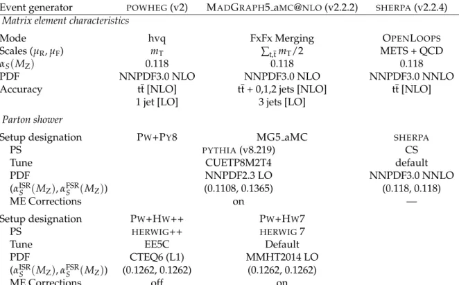
After performing the selection of the charged PF candidates we check which ones have been used in the clustering of the two b-tagged jets and which ones match the two charged lepton candidates within a∆R = √(∆η)2+ (∆φ)2 = 0.05 cone, where φ is the azimuthal angle in ra-dians. All PF candidates failing the kinematic requirements, being matched to another primary vertex in the event, or being matched to the charged leptons and b-tagged jets, are removed from the analysis. The UE analysis proceeds by using the remaining charged PF candidates. Figure 1 shows, in a simulated tt event, the contribution from charged and neutral PF candi-dates, the charged component of the pileup, and the hard process. The charged PF candidates that are used in the study of the UE are represented after applying the selection described above. −6 −4 −2 0 2 4 6 η −4 −3 −2 −1 0 1 2 3 φ [rad]

CMS Simulation t¯t→ (eνb)(µνb) (13 TeV)

Neutral PU charged

Charged Charged from b

Lepton

Figure 1: Distribution of all PF candidates reconstructed in a PW+PY8 simulated tt event in the η–φ plane. Only particles with pT > 900 MeV are shown, with a marker whose area is

proportional to the particle pT. The fiducial region in η is represented by the dashed lines.

Various characteristics, such as the multiplicity of the selected charged particles, the flux of momentum, and the topology or shape of the event have different sensitivity to the modeling of the recoil, the contribution from MPI and CR, and other parameters.

flux in the event:

• charged-particle multiplicity: N_ch;

• magnitude of the pTof the charged particle recoil system: |~pT| = |∑_iN=ch1~pT,i|;

• scalar sum of the pT(or pz) of charged particles:∑ pk=∑iN=ch1|~pk,i|, where k=T or z;

• average pT(or pz) per charged particle: computed from the ratio between the scalar

sum and the charged multiplicity: pT(or pz).

The second set of observables characterizes the UE shape and it is computed from the so-called linearized sphericity tensor [56, 57]:

Sµν ₌ Nch

∑

i=1 pµ i pνi/|pi| .Nch

∑

i=1 |p_i|, (1)

where the i index runs over the particles associated with the UE, as for the previous variables, and the µ and ν indices refer to one of the(x, y, z)components of the momentum of the parti-cles. The eigenvalues (λi) of Sµν are in decreasing order, i.e., with λ1 the largest one, and are

used to compute the following observables [58]:

• Aplanarity: A = 3₂λ3 measures the pT component out of the event plane, defined

by the two leading eigenvectors. Isotropic (planar) events are expected to have A= 1/2(0).

• Sphericity: S= 3₂(λ2+λ3)measures the p2_T with respect to the axis of the event. An

isotropic (dijet) event is expected to have S =1(0).

• C=3(λ1λ2+λ1λ3+λ2λ3)identifies 3 jet events (tends to be 0 for dijet events).

• D=27λ1λ2λ3identifies 4 jet events (tends to be 0 otherwise).

Further insight can be gained by studying the evolution of the two sets of observables in differ-ent categories of the tt system kinematic quantities. The categories chosen below are sensitive to the recoil or the scale of the energy of the hard process, and are expected to be reconstructed with very good resolution. Additionally, these variables minimize the effect of migration of events between categories due to resolution effects.

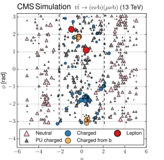
The dependence of the UE on the recoil system is studied in categories that are defined ac-cording to the multiplicity of additional jets with pT > 30 GeV and |η| < 2.5, excluding the two selected b-tagged jets. The categories with 0, 1, or more than 1 additional jet are used for this purpose. The additional jet multiplicity is partially correlated with the charged-particle multiplicity and helps to factorize the contribution from ISR. The distribution of the number of additional jets is shown in Fig. 2 (upper left).

In addition to these categories, the transverse momentum of the dilepton system, ~pT(``), is

used as it preserves some correlation with the transverse momentum of the tt system and, consequently, with the recoil of the system. The~pT(``)direction is used to define three regions

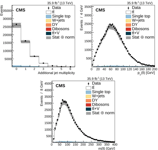
in the transverse plane of each event. The regions are denoted as “transverse” (60◦ < _|∆φ| < 120◦), “away” (|∆φ| > 120◦), and “toward” (|∆φ| < 60◦). Each reconstructed particle in an event is assigned to one of these regions, depending on the difference of their azimuthal angle with respect to the~pT(``)vector. Figure 3 illustrates how this classification is performed on

a typical event. This classification is expected to enhance the sensitivity of the measurements to the contributions from ISR, MPI and CR in different regions. In addition, the magnitude, pT(``), is used to categorize the events and its distribution is shown in Fig. 2 (upper right). The

0 1 2 3 4 5 6

Additional jet multiplicity 5000 10000 15000 20000 25000 30000 35000 Events Data t t Single top W+jets DY Dibosons +V t t norm ⊕ Stat CMS (13 TeV) -1 35.9 fb 0 20 40 60 80 100 120 140 160 180 200 (ll) [GeV] T p 500 1000 1500 2000 2500 3000 3500 Events / 4 GeV Data t t Single top W+jets DY Dibosons +V t t norm ⊕ Stat CMS (13 TeV) -1 35.9 fb 0 50 100 150 200 250 300 350 400 m(ll) [GeV] 500 1000 1500 2000 2500 3000 3500 4000 4500 Events / 8 GeV Data t t Single top W+jets DY Dibosons +V t t norm ⊕ Stat CMS (13 TeV) -1 35.9 fb

Figure 2: Distributions of the variables used to categorize the study of the UE. Upper left: multiplicity of additional jets (pT > 30 GeV). Upper right: pT(``). Lower: m(``). The

distri-butions in data are compared to the sum of the expectations for the signal and backgrounds. The shaded band represents the uncertainty associated to the integrated luminosity and the theoretical value of the tt cross section.

Lastly, the dependence of the UE on the energy scale of the hard process is characterized by measuring it in different categories of the m(``)variable. This variable is correlated with the invariant mass of the tt system, but not with its pT. The m(``)distribution is shown in Fig. 2

(lower). A resolution better than 2% is expected in the measurement of m(``).

Although both pT(``)and m(``)are only partially correlated with the tt kinematic quantities,

they are expected to be reconstructed with very good resolution. Because of the two escaping neutrinos, the kinematics of the tt pair can only be reconstructed by using the pmiss_T measure-ment, which has poorer experimental resolution when compared to the leptons. In addition, given that pmiss_T is correlated with the UE activity, as it stems from the balance of all PF candi-dates in the transverse plane, it could introduce a bias in the definition of the categories and the observables studied to characterize the UE. Hence the choice to use only dilepton-related variables. Toward, ~pT(``) Transverse Transverse Away Away

CMS Simulation t¯t→ (eνb)(µνb) (13 TeV)

Charged Lepton (pT/2)

Figure 3: Display of the transverse momentum of the selected charged particles, the two lep-tons, and the dilepton pair in the transverse plane corresponding to the same event as in Fig. 1. The pTof the particles is proportional to the length of the arrows and the dashed lines represent

the regions that are defined relative to the~pT(``)direction. For clarity, the pTof the leptons has

been rescaled by a factor of 0.5.

6

Corrections to the particle level

Inefficiencies of the track reconstruction due to the residual contamination from pileup, nuclear interactions in the tracker material, and accidental splittings of the primary vertex [59] are ex-pected to cause a slight bias in the observables described above. The correction for these biases is estimated from simulation and applied to the data by means of an unfolding procedure. At particle (generator) level, the distributions of the observables of interest are binned accord-ing to the resolutions expected from simulation. Furthermore, we require that each bin con-tains at least 2% of the total number of events. The migration matrix (K), used to map the reconstruction- to particle-level distributions, is constructed using twice the number of bins at the reconstruction level than the ones used at particle level. This procedure ensures almost diagonal matrices, which have a numerically stable inverse. The matrix is extended with an

additional row that is used to count the events failing the reconstruction-level requirements, but found in the fiducial region of the analysis, i.e., passing the particle-level requirements. The inversion of the migration matrix is made using a Tikhonov regularization procedure [60], as implemented in the TUNFOLDDENSITYpackage [61]. The unfolded distribution is found by minimizing a χ2function

χ2 = (y−Kλ)TV_yy−1(y−Kλ) +τ2||L(λ−λ0)||2, (2)

where y are the observations, Vyy is an estimate of the covariance of y (calculated using the

simulated signal sample), λ is the particle-level expectation,||L(λ−λ0)||2is a penalty function

(with λ0 being estimated from the simulated samples), and τ > 0 is the so-called

regulariza-tion parameter. The latter regulates how strongly the penalty term should contribute to the minimization of χ2. In our setup we choose the function L to be the curvature, i.e., the second derivative, of the output distribution. The chosen value of the τ parameter is optimized for each distribution by minimizing its average global correlation coefficient [61]. Small values, i.e., τ < 10−3, are found for all the distributions; the global correlation coefficients are around 50%. After unfolding, the distributions are normalized to unity.

The statistical coverage of the unfolding procedure is checked by means of pseudo-experiments based on independent PW+PY8 samples. The pull of each bin in each distribution is found to be consistent with that of a standard normal distribution. The effect of the regularization term in the unfolding is checked in the data by folding the measured distributions and comparing the outcome to the originally-reconstructed data. In general the folded and the original distri-butions agree within 1–5% in each bin, with the largest differences observed in bins with low yield.

7

Systematic uncertainties

The impact of different sources of uncertainty is evaluated by unfolding the data with alter-native migration matrices, which are obtained after changing the settings in the simulations as explained below. The effect of a source of uncertainty in non-fiducial tt events is included in this estimate, by updating the background prediction. The observed bin-by-bin differences are used as estimates of the uncertainty. The impact of the uncertainty in the background normalization is the only exception to this procedure, as detailed below. The covariance matrices associated to each source of uncertainty are built using the procedure described in detail in [62]. In case several sub-contributions are used to estimate a source of uncertainty, the corresponding dif-ferences in each bin are treated independently, symmetrized, and used to compute individual covariance matrices, which preserve the normalization. Variations on the event yields are fully absorbed by normalizing the measured cross sections. Thus, only the sources of uncertainty that yield variations in the shapes have a non-negligible impact.

7.1 Experimental uncertainties

The following experimental sources of uncertainty are considered:

Pileup: Although pileup is included in the simulation, there is an intrinsic uncertainty in mod-eling its multiplicity. An uncertainty of_±4.6% in the inelastic pp cross section is used and propagated to the event weights [63].

Trigger and selection efficiency: The scale factors used to correct the simulation for different trigger and lepton selection efficiencies in data and simulation are varied up or down,

according to their uncertainty. The uncertainties in the muon track and electron recon-struction efficiencies are included in this category and added in quadrature.

Lepton energy scale: The corrections applied to the electron energy and muon momentum scales are varied separately, according to their uncertainties. The corrections and uncer-tainties are obtained using methods similar to those described in Refs. [64, 65]. These variations lead to a small migration of events between the different pT(``)or m(``)

cate-gories used in the analysis.

Jet energy scale: A pT- and η-dependent parameterization of the jet energy scale is used to

vary the calibration of the jets in the simulation. The corrections and uncertainties are obtained using methods similar to those described in Ref. [51]. The effect of these varia-tions is similar to that described for the lepton energy scale uncertainty; in this case the migration of events occurs between different jet multiplicity categories.

Jet energy resolution: Each jet is further smeared up or down depending on its pTand η, with

respect to the central value measured in data. The difference with respect to data is mea-sured using methods similar to those described in Ref. [51]. The main effect induced in the analysis from altering the jet energy resolution is similar to that described for the jet energy scale uncertainty.

b tagging and misidentification efficiencies: The scale factors used to correct for the differ-ence in performance between data and simulation are varied according to their uncer-tainties and depending on the flavor of the jet [52]. The main effect of this variation is to move jets into the candidate b jets sample or remove them from it.

Background normalization: The impact of the uncertainty in the normalization of the back-grounds is estimated by computing the difference obtained with respect to the nominal result when these contributions are not subtracted from data. This difference is expected to cover the uncertainty in the normalization of the main backgrounds, i.e., DY and the tW process, and the uncertainty in the normalization of the tt events that are expected to pass the reconstruction-level requirements but fail the generator-level ones. The total expected background contribution is at the level of 8–10%, depending on the bin. The impact from this uncertainty is estimated to be<5%.

Tracking reconstruction efficiency: The efficiency of track reconstruction is found to be more than 90%. It is monitored using muon candidates from Z _→ µ+µ−decays, and the ra-tio of the four-body final D0 _{→ K}−_π+

π−π+decay to the two-body D0 → K−π+ decay. The latter is used to determine a data-to-simulation scale factor (SFtrk) as a function of

the pseudorapidity of the tracks, and for different periods of the data taking used in this analysis. The envelope of the SFtrk values, with uncertainties included, ranges from 0.89

to 1.17 [66], and it provides an adequate coverage for the residual variations observed in the charged-particle multiplicity between different data taking periods. The impact of the variation of SFtrk by its uncertainty is estimated by using the value of|1−SFtrk|for the

probability to remove a reconstructed track from the event or to promote an unmatched generator-level charged particle to a reconstructed track, depending on whether SF_trk <1 or>1, respectively. Different migration matrices, reflecting the different tracking efficien-cies obtained from varying the uncertainty in SFtrk, are obtained by this method and used

to unfold the data. Although the impact is nonnegligible on variables such as Nchor∑ pT,

7.2 Theoretical uncertainties

The following theoretical uncertainties are considered:

Scale choices: µR and µF are varied individually in the ME by factors between 0.5 and 2,

ex-cluding the extreme cases µR/µF = µ(2, 0.5)and µ(0.5, 2), according to the prescription described in Refs. [67, 68].

Resummation scale and αSused in the parton shower: InPOWHEG, the real emission cross

sec-tion is scaled by a damping funcsec-tion, parameterized by the so-called hdampvariable [13–

15]. This parameter controls the ME-PS matching and regulates the high-pT radiation by

reducing real emissions generated byPOWHEG with a factor of h2_damp/(p2_T+h2_damp). In the simulation used to derive the migration matrices, h_damp =1.58 mtand the uncertainty

in this value is evaluated by changing it by +42 or -37%, a range that is determined from the jet multiplicity measurements in tt at√s = 8 TeV [20]. Likewise, the uncertainty as-sociated with the choice of αISR_S (MZ) =0.1108 for space-like and αFSRS (MZ) = 0.1365 for

time-like showers in the CUETP8M2T4 tune is evaluated by varying the scale at which it is computed, MZ, by a factor of 2 or 1/2.

UE model: The dependence of the migration matrix on the UE model assumed in the simula-tion is tested by varying the parameters that model the MPI and CR in the range of values corresponding to the uncertainty envelope associated to the CUETP8M2T4 tune. The un-certainty envelope has been determined using the same methods as described in Ref. [19]. In the following, these will be referred to as UE up/down variations. The dependence on the CR model is furthermore tested using other models besides the nominal one, which is the MPI-based CR model where the tt decay products are excluded from reconnections to the UE. A dedicated sample where the reconnections to resonant decay products are enabled (hereafter designated as ERDon) is used to evaluate possible differences in the unfolded results. In addition, alternative models for the CR are tested. One sample uti-lizing the “gluon move” model [5], in which gluons can be moved to another string, and another utilizing the “QCD-based” model with string formation beyond LO [32] are used for this purpose. In both samples, the reconnections to the decay resonant processes are enabled. The envelope of the differences is considered as a systematic uncertainty. t quark pT: The effect of reweighting of the simulated t quark pT (pT(t)) distribution to match

the one reconstructed from data [69, 70] is added as an additional uncertainty. This has the most noticeable effect on the fraction of events that do not pass the reconstruction-level requirements and migrate out of the fiducial phase space.

t quark mass: An additional uncertainty is considered, related to the value of mt = 172.5 GeV

used in the simulations, by varying this parameter by±0.5 GeV [71].

Any possible uncertainty from the choice of the hadronization model is expected to be signif-icantly smaller than the theory uncertainties described above. This has been explicitly tested by comparing the results at reconstruction level and after unfolding the data with the PW+PY8 and PW+HW++ migration matrices. The latter relies on a different hadronization model, but it folds other modelling differences such as the underlying event tune or the parton shower as well. Thus it can only be used as a test setup to validate the measurement.

7.3 Summary of systematic uncertainties

The uncertainties on the measurement of the normalized differential cross sections are domi-nated by the systematic uncertainties, although in some bins of the distributions the statistical uncertainties are a large component. The experimental uncertainties have, in general, small impact; the most relevant are the tracking reconstruction efficiency for the Nch,∑ pT,∑ pz, and

|~pT|observables. Other observables are affected at a sub-percent level by this uncertainty.

The-ory uncertainties affect the measurements more significantly, a fact that underlines the need of better tuning of the model parameters.

Event shape observables are found to be the most robust against this uncertainty, while∑ pT,

∑ pz, and|~pT| are the ones that suffer more from it. Other sources of theoretical uncertainty

typically have a smaller effect.

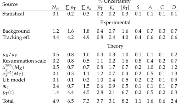
To further illustrate the impact of different sources on the observables considered, we list in Table 2 the uncertainties on the average of each observable. In the table, only systematic uncer-tainties that impact the average of one of the observables by at least 0.5% are included. The total uncertainty on the average of a given quantity ranges from 1 to 8%, and hence the comparison with model predictions can be carried out in a discrete manner.

Table 2: Uncertainties affecting the measurement of the average of the UE observables. The values are expressed in % and the last row reports the quadratic sum of the individual contri-butions. Source % Uncertainty N_{ch ∑ p}T ∑ pz pT pz |~pT| S A C D Statistical 0.1 0.2 0.3 0.2 0.2 0.3 0.1 0.1 0.1 0.1 Experimental Background 1.2 1.6 1.8 0.4 0.7 1.6 0.4 0.7 0.3 0.7 Tracking eff. 4.4 4.2 4.9 0.8 0.4 4.0 0.4 0.6 0.2 0.6 Theory µR/µF 0.5 0.8 1.0 0.3 0.3 1.0 0.1 0.1 0.1 0.2 Resummation scale 0.2 0.8 0.5 1.1 0.2 1.6 0.8 0.4 0.2 0.7 αFSR_S (MZ) 0.5 0.7 0.7 0.8 1.7 0.7 0.2 1.0 0.2 1.2 αISR_S (MZ) 0.1 0.3 1.1 1.2 0.7 0.4 0.2 0.5 0.1 1.3 UE model 0.1 0.1 0.2 1.0 0.4 0.5 0.2 0.2 0.1 0.9 mt 0.4 0.7 1.5 0.6 0.9 0.5 0.1 0.1 0.1 0.7 pT(t) 1.4 4.4 4.5 2.8 2.1 6.7 0.2 0.5 0.2 0.3 Total 4.9 6.5 7.3 3.7 3.1 8.2 1.1 1.6 0.6 2.4

8

Results

8.1 Inclusive distributions

The normalized differential cross sections measured as functions of Nch, ∑ pT, pT, |~pT|, ∑ pz,

pz, sphericity, aplanarity, C, and D are shown in Figs. 4–13, respectively. The distributions are

obtained after unfolding the background-subtracted data and normalizing the result to unity. The result is compared to the simulations, whose settings are summarized in Table 1 and in the appendix. For the predictions, the statistical uncertainty is represented as an error bar. In the specific case of the PW+PY8 setup, the error bar represents the envelope obtained by

varying the main parameters of the CUETP8M2T4 tune, according to their uncertainties. The envelope includes the variation of the CR model, αISR_S (MZ), αFSR_S (MZ), the hdamp parameter,

and the µR/µFscales at the ME level. Thus, the uncertainty band represented for the PW+PY8

setup should be interpreted as the theory uncertainty in that prediction. For each distribution we give, in addition, the ratio between different predictions and the data.

In tt events the UE contribution is determined to have typicallyO(20)charged particles with pT ∼ pz ≈ 2 GeV, vectorially summing to a recoil of about 10 GeV. The distribution of the

UE activity is anisotropic (as the sphericity is < 1), close to planar (as the aplanarity peaks at low values of_≈0.1), and peaks at around 0.75 in the C variable, which identifies three-jet topologies. The D variable, which identifies the four-jet topology, is instead found to have values closer to 0. The three-prong configuration in the energy flux of the UE described by the C variable can be identified with two of the eigenvectors of the linearized sphericity tensor being correlated with the direction of the b-tagged jets, and the third one being determined by energy conservation. When an extra jet with pT > 30 GeV is selected, we measure a change in

the profile of the event shape variables, with average values lower by 20–40% with respect to the distributions in which no extra jet is found. Thus when an extra jet is present, the event has a dijet-like topology instead of an isotropic shape.

The results obtained with PYTHIA8 for the parton shower simulation show negligible depen-dence on the ME generator with which it is interfaced, i.e., PW+PY8 and MG5 aMC yield similar results. In all distributions the contribution from MPI is strong: switching off this com-ponent in the simulation has a drastic effect on the predictions of all the variables analyzed. Color reconnection effects are more subtle to identify in the data. In the inclusive distributions, CR effects are needed to improve the theory accuracy for pT < 3 GeV or pz < 5 GeV. The

differences between the CR models tested (as discussed in detail in Section 3) are neverthe-less small and almost indistinguishable in the inclusive distributions. In general the PW+PY8 setup is found to be in agreement with the data, when the total theory uncertainty is taken into account. In most of the distributions it is the variation of αFSR

S (MZ) that dominates the

the-ory uncertainty, as this variation leads to the most visible changes in the UE. The other parton shower setups tested do not describe the data as accurately, but they were not tuned to the same level of detail as PW+PY8. The PW+HW++ and PW+HW7-based setups show distinct trends with respect to the data from those observed in any of thePYTHIA8-based setups. While describing fairly well the UE event shape variables,HERWIG++ andHERWIG 7 disagree with the Nch, pT, and pz measurements. The SHERPApredictions disagree with data in most of the

observables.

For each distribution the level of agreement between theory predictions and data is quantified by means of a χ2variable defined as:

χ2=

n

∑

i,j=1

δyi(Cov−1)ijδyj, (3)

where δyi (δyj) are the differences between the data and the model in the i-th (j-th) bin; here n

represents the total number of bins, and Cov−1 is the inverse of the covariance matrix. Given that the distributions are normalized, the covariance matrix becomes invertible after removing its first row and column. In the calculation of Eq. 3 we assume that the theory uncertainties are uncorrelated with those assigned to the measurements. Table 3 summarizes the values ob-tained for the main models with respect to each of the distributions shown in Figs. 4–13. The values presented in the table quantify the level of agreement of each model with the measure-ments. Low χ2 _{per number of degrees of freedom (dof) values are obtained for the PW+PY8}

ch

N

0

20

40

60

80

100

120

)

ch

1/N dN/d(N

0

0.02

0.04

0.06

0.08

Data PW+PY8 ISR up ISR down FSR up FSR down UE up UE down

CMS

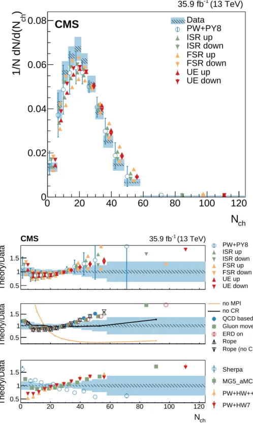
(13 TeV) -1 35.9 fb Theory/Data 0.5 1 1.5 CMS 35.9 fb-1 (13 TeV) PW+PY8 ISR up ISR down FSR up FSR down UE up UE down Theory/Data 0.5 1 1.5 no MPI no CR QCD based Gluon move ERD on Rope Rope (no CR) ch N 0 20 40 60 80 100 120 Theory/Data 0.5 1 1.5 Sherpa MG5_aMC PW+HW++ PW+HW7

Figure 4: The normalized differential cross section as a function of N_ch is shown on the upper panel. The data (colored boxes) are compared to the nominal PW+PY8 predictions and to the expectations obtained from varied αISR_S (MZ)or α_SFSR(MZ)PW+PY8 setups (markers). The

dif-ferent panels on the lower display show the ratio between each model tested (see text) and the data. In both cases the shaded (hatched) band represents the total (statistical) uncertainty of the data, while the error bars represent either the total uncertainty of the PW+PY8 setup, computed as described in the text, or the statistical uncertainty of the other MC simulation setups.

[GeV]

T

p

Σ

2 3 4 5

10

20

10

2

2

×

10

2

]

-1

) [GeV

_T

p

Σ

1/N dN/d(

0

0.01

0.02

0.03

Data PW+PY8 ISR up ISR down FSR up FSR down UE up UE down

CMS

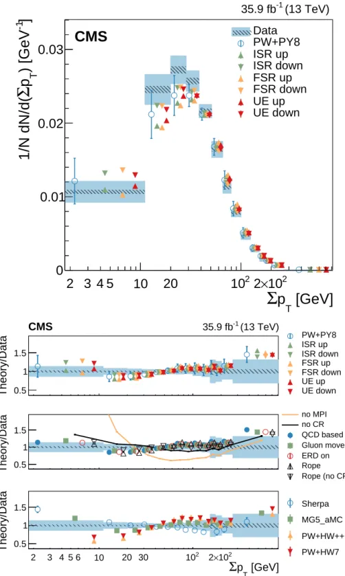
(13 TeV) -1 35.9 fb Theory/Data 0.5 1 1.5 CMS 35.9 fb-1 (13 TeV) PW+PY8 ISR up ISR down FSR up FSR down UE up UE down Theory/Data 0.5 1 1.5 no MPI no CR QCD based Gluon move ERD on Rope Rope (no CR) [GeV] T p

Σ

2 3 4 5 6 10 20 30 102 2×102 Theory/Data 0.5 1 1.5 Sherpa MG5_aMC PW+HW++ PW+HW7

Figure 5: Normalized differential cross section as function of∑ pT, compared to the predictions

[GeV]

T

p

1

2

3

4 5 6 7 8 910

20

]

-1

) [GeV

_T

p

1/N dN/d(

0

0.5

1

1.5

2

Data PW+PY8 ISR up ISR down FSR up FSR down UE up UE down

CMS

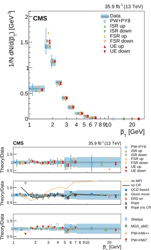
(13 TeV) -1 35.9 fb Theory/Data 0.5 1 1.5 CMS 35.9 fb-1 (13 TeV) PW+PY8 ISR up ISR down FSR up FSR down UE up UE down Theory/Data 0.5 1 1.5 no MPI no CR QCD based Gluon move ERD on Rope Rope (no CR) [GeV] T p 1 2 3 4 5 6 7 8 910 20 Theory/Data 0.5 1 1.5 Sherpa MG5_aMC PW+HW++ PW+HW7

Figure 6: Normalized differential cross section as function of pT, compared to the predictions

| [GeV]

T

p

|

1

2 3 4 5

10

20

10

2

2

×

10

2

]

-1

|) [GeV

_T

p

1/N dN/d(|

0

0.02

0.04

0.06

0.08

DataPW+PY8 ISR up ISR down FSR up FSR down UE up UE down

CMS

(13 TeV) -1 35.9 fb Theory/Data 0.5 1 1.5 CMS 35.9 fb-1 (13 TeV) PW+PY8 ISR up ISR down FSR up FSR down UE up UE down Theory/Data 0.5 1 1.5 no MPI no CR QCD based Gluon move ERD on Rope Rope (no CR) | [GeV] T p | 1 2 3 4 5 6 10 20 30 102 2×102 Theory/Data 0.5 1 1.5 Sherpa MG5_aMC PW+HW++ PW+HW7

Figure 7: Normalized differential cross section as function of|~pT|, compared to the predictions

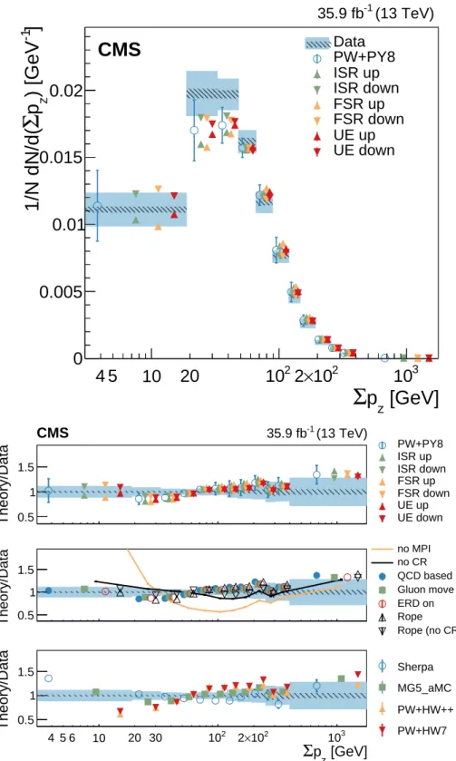
[GeV]

z

p

Σ

4 5

10

20

10

2

2

×

10

2

10

3

]

-1

) [GeV

_z

p

Σ

1/N dN/d(

0

0.005

0.01

0.015

0.02

Data PW+PY8 ISR up ISR down FSR up FSR down UE up UE down

CMS

(13 TeV) -1 35.9 fb Theory/Data 0.5 1 1.5 CMS 35.9 fb-1 (13 TeV) PW+PY8 ISR up ISR down FSR up FSR down UE up UE down Theory/Data 0.5 1 1.5 no MPI no CR QCD based Gluon move ERD on Rope Rope (no CR) [GeV] z p

Σ

4 5 6 10 20 30 102 2×102 103 Theory/Data 0.5 1 1.5 Sherpa MG5_aMC PW+HW++ PW+HW7

Figure 8: Normalized differential cross section as function of∑ pz, compared to the predictions

[GeV]

z

p

1

2

3 4 5 6 7

10

20

30 40

]

-1

) [GeV

_z

p

1/N dN/d(

0

0.2

0.4

0.6

0.8

Data PW+PY8 ISR up ISR down FSR up FSR down UE up UE down

CMS

(13 TeV) -1 35.9 fb Theory/Data 0.5 1 1.5 CMS 35.9 fb-1 (13 TeV) PW+PY8 ISR up ISR down FSR up FSR down UE up UE down Theory/Data 0.5 1 1.5 no MPI no CR QCD based Gluon move ERD on Rope Rope (no CR) [GeV] z p 1 2 3 4 5 6 7 8 910 20 30 40 50 Theory/Data 0.5 1 1.5 Sherpa MG5_aMC PW+HW++ PW+HW7

Figure 9: Normalized differential cross section as function of pz, compared to the predictions

S

0

0.1 0.2 0.3 0.4 0.5 0.6 0.7 0.8 0.9

1

1/N dN/dS

0

2

4

Data PW+PY8 ISR up ISR down FSR up FSR down UE up UE down

CMS

(13 TeV) -1 35.9 fb Theory/Data 0.5 1 1.5 CMS 35.9 fb-1 (13 TeV) PW+PY8 ISR up ISR down FSR up FSR down UE up UE down Theory/Data 0.5 1 1.5 no MPI no CR QCD based Gluon move ERD on Rope Rope (no CR) S 0 0.1 0.2 0.3 0.4 0.5 0.6 0.7 0.8 0.9 1 Theory/Data 0.5 1 1.5 Sherpa MG5_aMC PW+HW++ PW+HW7

Figure 10: Normalized differential cross section as function of the sphericity variable, compared to the predictions of different models. The conventions of Fig. 4 are used.

A

0 0.05 0.1 0.15 0.2 0.25 0.3 0.35 0.4 0.45 0.5

1/N dN/dA

0

5

10

Data PW+PY8 ISR up ISR down FSR up FSR down UE up UE down

CMS

(13 TeV) -1 35.9 fb Theory/Data 0.5 1 1.5 CMS 35.9 fb-1 (13 TeV) PW+PY8 ISR up ISR dn FSR up FSR dn UE up UE dn Theory/Data 0.5 1 1.5 no MPI no CR QCD based Gluon move ERD on Rope Rope (no CR) Aplanarity 0 0.05 0.1 0.15 0.2 0.25 0.3 0.35 0.4 0.45 0.5 Theory/Data 0.5 1 1.5 Sherpa aMC@NLO+PY8 PW+HW++ PW+HW7

Figure 11: Normalized differential cross section as function of the aplanarity variable, com-pared to the predictions of different models. The conventions of Fig. 4 are used.

C

0

0.1 0.2 0.3 0.4 0.5 0.6 0.7 0.8 0.9

1

1/N dN/dC

0

2

4

Data PW+PY8 ISR up ISR down FSR up FSR down UE up UE down

CMS

(13 TeV) -1 35.9 fb Theory/Data 0.5 1 1.5 CMS 35.9 fb-1 (13 TeV) PW+PY8 ISR up ISR down FSR up FSR down UE up UE down Theory/Data 0.5 1 1.5 no MPI no CR QCD based Gluon move ERD on Rope Rope (no CR) C 0 0.1 0.2 0.3 0.4 0.5 0.6 0.7 0.8 0.9 1 Theory/Data 0.5 1 1.5 Sherpa MG5_aMC PW+HW++ PW+HW7

Figure 12: Normalized differential cross section as function of the C variable, compared to the predictions of different models. The conventions of Fig. 4 are used.

D

0

0.1 0.2 0.3 0.4 0.5 0.6 0.7 0.8 0.9

1

1/N dN/dD

0

2

4

6

Data PW+PY8 ISR up ISR down FSR up FSR down UE up UE down

CMS

(13 TeV) -1 35.9 fb Theory/Data 0.5 1 1.5 CMS 35.9 fb-1 (13 TeV) PW+PY8 ISR up ISR down FSR up FSR down UE up UE down Theory/Data 0.5 1 1.5 no MPI no CR QCD based Gluon move ERD on Rope Rope (no CR) D 0 0.1 0.2 0.3 0.4 0.5 0.6 0.7 0.8 0.9 1 Theory/Data 0.5 1 1.5 Sherpa MG5_aMC PW+HW++ PW+HW7

Figure 13: Normalized differential cross section as function of the D variable, compared to the predictions of different models. The conventions of Fig. 4 are used.

setup when all the theory uncertainties of the model are taken into account, in particular for the event shape variables. This indicates that the theory uncertainty envelope is conservative. Table 3: Comparison between the measured distributions at particle level and the predictions of different generator setups. We list the results of the χ2 tests together with dof. For the comparison no uncertainties in the predictions are taken into account, except for the PW+PY8 setup for which the comparison including the theoretical uncertainties is quoted separately in parenthesis. Observable χ 2_/dof PW+PY8 PW+HW++ PW+HW7 MG5 aMC SHERPA Nch 30/11 (15/11) 33/11 17/11 34/11 95/11 ∑ pT 24/13 (13/13) 129/13 56/13 30/13 37/13 ∑ pz 8/11 (4/11) 34/11 20/11 9/11 18/11 pT 12/9 (1/9) 40/9 56/9 6/9 56/9 pz 2/9 (1/9) 9/9 32/9 1/9 36/9 |~pT| 17/11 (7/11) 102/11 49/11 20/11 34/11 S 29/7 (3/7) 7/7 17/7 36/7 194/7 A 18/7 (1/7) 8/7 13/7 26/7 167/7 C 34/7 (4/7) 7/7 27/7 38/7 187/7 D 7/7 (1/7) 5/7 8/7 11/7 83/7

8.2 Profile of the UE in different categories

The differential cross sections as functions of different observables are measured in different event categories introduced in Section 5. We report the profile, i.e., the average of the measured differential cross sections in different event categories, and compare it to the expectations from the different simulation setups. Figures 14–23 summarize the results obtained. Additional results for pT, profiled in different categories of pT(``)and/or jet multiplicity, are shown in

Figs. 24 and 25, respectively. In all figures, the pull of the simulation distributions with re-spect to data, defined as the difference between the model and the data divided by the total uncertainty, is used to quantify the level of agreement.

The average charged-particle multiplicity and the average of the momentum flux observables vary significantly when extra jets are found in the event or for higher pT(``)values. The same

set of variables varies very slowly as a function of m(``). Event shape variables are mostly affected by the presence of extra jets in the event, while varying slowly as a function of pT(``)

or m(``). The average sphericity increases significantly when no extra jets are present in the event showing that the UE is slightly more isotropic in these events. A noticeable change is also observed for the other event shape variables in the same categories.

For all observables, the MPI contribution is crucial: most of the pulls are observed to be larger than 5 when MPI is switched off in the simulation. Color reconnection effects are on the other hand more subtle and are more relevant for pT, specifically when no additional jet is present

in the event. This is illustrated by the fact that the pulls of the setup without CR are larger for events belonging to these categories. Event shape variables also show sensitivity to CR. All other variations of the UE and CR models tested yield smaller variations of the pulls, compared to the ones discussed.

Although a high pull value of the PW+PY8 simulation is obtained for several categories, when different theory variations are taken into account, the envelope encompasses the data. The variations of αFSR_S (MZ)and αISR_S (MZ)account for the largest contribution to this envelope. As

already noted in the previous section, the PW+HW++, PW+HW7, andSHERPAmodels tend to be in worse agreement with data than PW+PY8, indicating that further tuning of the first two is needed.

8.3 Sensitivity to the choice of αS in the parton shower

The sensitivity of these results to the choice of αS(MZ)in the parton shower is tested by

per-forming a scan of the χ2value defined by Eq. (3), as a function of αISR_S (MZ)or αFSR_S (MZ). The

χ2is scanned fixing all the other parameters of the generator. A more complete treatment could only be achieved with a fully tuned UE, which lies beyond the scope of this paper. While no sensitivity is found to αISR_S (MZ), most observables are influenced by the choice of αFSRS (MZ).

The most sensitive variable is found to be pT and the corresponding variation of the χ2

func-tion is reported in Fig. 26. A polynomial interpolafunc-tion is used to determine the minimum of the scan (best fit), and the points at which the χ2_{function increases by one unit are used to derive}

the 68% confidence interval (CI). The degree of the polynomial is selected by a stepwise regres-sion based on an F-test statistics [72]. A value of αFSR_S (MZ) =0.120±0.006 is obtained, which is

lower than the one assumed in the Monash tune [73] and used in the CUETP8M2T4 tune. The value obtained is compatible with the one obtained from the differential cross sections mea-sured as a function of pT in different pT(``)regions or in events with different additional jet

multiplicities. Table 4 summarizes the results obtained. From the inclusive results, we conclude that the range of the energy scale that corresponds to the 5% uncertainty attained in the deter-mination of αFSR

S (MZ)can be approximated by a[

√

2, 1/√2]variation, improving considerably over the canonical[2, 0.5]scale variations.

Table 4: The first rows give the best fit values for αFSR_S for the PW+PY8 setup, obtained from the inclusive distribution of different observables and the corresponding 68 and 95% confidence intervals. The last two rows give the preferred value of the renormalization scale in units of MZ,

and the associated_±1σ interval that can be used as an estimate of its variation to encompass the differences between data and the PW+PY8 setup.

p_T

(``)

region Inclusive Away Toward Transverse

Best fit αFSR_S

(

MZ

)

0.120 0.119 0.116 0.119

68% CI [-0.006,+0.006] [-0.011,+0.010] [-0.013,+0.011] [-0.006,+0.006] 95% CI [-0.013,+0.011] [-0.022,+0.019] [-0.030,+0.021] [-0.013,+0.012]

µ_R/M_Z 2.3 2.4 2.9 2.4

Category

Inc. =0 =1 ≥2 [0,20[ [20,40[[40,80[[80,120[>120 [0,60[ [60,120[[120,200[>200

〉

ch

N

〈

10

20

30

40

50

60

Data PW+PY8

ISR up ISR down

FSR up FSR down

UE up UE down

Extra jets (ll) [GeV]

T p m(ll) [GeV]

CMS

35.9 fb-1 (13 TeV) Data σ (Theory-Data) −4 2 −0 2 4 CMS 35.9 fb-1 (13 TeV) PW+PY8 ISR up ISR down FSR up FSR down UE up UE down Data σ (Theory-Data) 4 − 2 − 0 2 4 no MPI_{no CR} QCD based Gluon move ERD on Rope Rope (no CR)

Category

Inc. =0 =1 ≥2 [0,20[ [20,40[ [40,80[ [80,120[>120 [0,60[ [60,120[[120,200[>200 Data σ (Theory-Data) −4 2 − 0 2 4 Sherpa MG5_aMC PW+HW++ PW+HW7

Extra jets (ll) [GeV]

T

p m(ll) [GeV]

Figure 14: Average Nch in different event categories. The mean observed in data (boxes) is

compared to the predictions from different models (markers), which are superimposed in the upper figure. The total (statistical) uncertainty of the data is represented by a shaded (hatched) area and the statistical uncertainty of the models is represented with error bars. In the specific case of the PW+PY8 model the error bars represent the total uncertainty (see text). The lower figure displays the pull between different models and the data, with the different panels corre-sponding to different sets of models. The bands represent the interval where|pull| < 1. The error bar for the PW+PY8 model represents the range of variation of the pull for the different configurations described in the text.

Category

Inc. =0 =1 ≥2 [0,20[ [20,40[[40,80[[80,120[>120 [0,60[ [60,120[[120,200[>200

[GeV]

〉

T

p

Σ

〈

20

40

60

80

100

120

140

160

180

200

_{Data PW+PY8}

ISR up ISR down

FSR up FSR down

UE up UE down

Extra jets p_T(ll) [GeV] m(ll) [GeV]

CMS

35.9 fb-1 (13 TeV) Data σ (Theory-Data) −4 2 − 0 2 4 CMS 35.9 fb-1 (13 TeV) PW+PY8 ISR up ISR down FSR up FSR down UE up UE down Data σ (Theory-Data) 4 − 2 − 0 2 4 no MPI_{no CR} QCD based Gluon move ERD on Rope Rope (no CR)

Category

Inc. =0 =1 ≥2 [0,20[ [20,40[ [40,80[ [80,120[>120 [0,60[ [60,120[[120,200[>200 Data σ (Theory-Data) −4 2 − 0 2 4 Sherpa MG5_aMC PW+HW++ PW+HW7

Extra jets p_T(ll) [GeV] m(ll) [GeV]

Category

Inc. =0 =1 ≥2 [0,20[ [20,40[[40,80[[80,120[>120 [0,60[ [60,120[[120,200[>200

[GeV]

〉

z

p

Σ

〈

50

100

150

200

250

Data_{ISR up} PW+PY8_{ISR down}

FSR up FSR down

UE up UE down

Extra jets p_T(ll) [GeV] m(ll) [GeV]

CMS

35.9 fb-1 (13 TeV) Data σ (Theory-Data) −4 2 − 0 2 4 CMS 35.9 fb-1 (13 TeV) PW+PY8 ISR up ISR down FSR up FSR down UE up UE down Data σ (Theory-Data) 4 − 2 − 0 2 4 no MPI_{no CR} QCD based Gluon move ERD on Rope Rope (no CR)

Category

Inc. =0 =1 ≥2 [0,20[ [20,40[ [40,80[ [80,120[>120 [0,60[ [60,120[[120,200[>200 Data σ (Theory-Data) −4 2 − 0 2 4 Sherpa MG5_aMC PW+HW++ PW+HW7

Extra jets p_T(ll) [GeV] m(ll) [GeV]

Category

Inc. =0 =1 ≥2 [0,20[ [20,40[[40,80[[80,120[>120 [0,60[ [60,120[[120,200[>200

[GeV]

〉

T

p

〈

1.5

2

2.5

3

3.5

4

4.5

5

Data PW+PY8

ISR up ISR down

FSR up FSR down

UE up UE down

Extra jets p_T(ll) [GeV] m(ll) [GeV]

CMS

35.9 fb-1 (13 TeV) Data σ (Theory-Data) −4 2 − 0 2 4 CMS 35.9 fb-1 (13 TeV) PW+PY8 ISR up ISR down FSR up FSR down UE up UE down Data σ (Theory-Data) 4 − 2 − 0 2 4 no MPI_{no CR} QCD based Gluon move ERD on Rope Rope (no CR)

Category

Inc. =0 =1 ≥2 [0,20[ [20,40[ [40,80[ [80,120[>120 [0,60[ [60,120[[120,200[>200 Data σ (Theory-Data) −4 2 − 0 2 4 Sherpa MG5_aMC PW+HW++ PW+HW7

Extra jets p_T(ll) [GeV] m(ll) [GeV]

Category

Inc. =0 =1 ≥2 [0,20[ [20,40[[40,80[[80,120[>120 [0,60[ [60,120[[120,200[>200

〉

z

p

〈

3

4

5

6

7

Data PW+PY8

ISR up ISR down

FSR up FSR down

UE up UE down

Extra jets p_T(ll) [GeV] m(ll) [GeV]

CMS

35.9 fb-1 (13 TeV) Data σ (Theory-Data) −4 2 − 0 2 4 CMS 35.9 fb-1 (13 TeV) PW+PY8 ISR up ISR down FSR up FSR down UE up UE down Data σ (Theory-Data) 4 − 2 − 0 2 4 no MPI_{no CR} QCD based Gluon move ERD on Rope Rope (no CR)

Category

Inc. =0 =1 ≥2 [0,20[ [20,40[ [40,80[ [80,120[>120 [0,60[ [60,120[[120,200[>200 Data σ (Theory-Data) −4 2 − 0 2 4 Sherpa MG5_aMC PW+HW++ PW+HW7

Extra jets p_T(ll) [GeV] m(ll) [GeV]

Category

Inc. =0 =1 ≥2 [0,20[ [20,40[[40,80[[80,120[>120 [0,60[ [60,120[[120,200[>200

[GeV]

〉

|

_T

p |

〈

20

40

60

80

100

Data PW+PY8

ISR up ISR down

FSR up FSR down

UE up UE down

Extra jets p_T(ll) [GeV] m(ll) [GeV]

CMS

35.9 fb-1 (13 TeV) Data σ (Theory-Data) −4 2 − 0 2 4 CMS 35.9 fb-1 (13 TeV) PW+PY8 ISR up ISR down FSR up FSR down UE up UE down Data σ (Theory-Data) 4 − 2 − 0 2 4 no MPI_{no CR} QCD based Gluon move ERD on Rope Rope (no CR)

Category

Inc. =0 =1 ≥2 [0,20[ [20,40[ [40,80[ [80,120[>120 [0,60[ [60,120[[120,200[>200 Data σ (Theory-Data) −4 2 − 0 2 4 Sherpa MG5_aMC PW+HW++ PW+HW7

Extra jets p_T(ll) [GeV] m(ll) [GeV]

Category

Inc. =0 =1 ≥2 [0,20[ [20,40[[40,80[[80,120[>120 [0,60[ [60,120[[120,200[>200

〉

S

〈

0.3

0.35

0.4

0.45

0.5

0.55

0.6

Data PW+PY8

ISR up ISR down

FSR up FSR down

UE up UE down

Extra jets p_T(ll) [GeV] m(ll) [GeV]

CMS

35.9 fb-1 (13 TeV) Data σ (Theory-Data) −4 2 − 0 2 4 CMS 35.9 fb-1 (13 TeV) PW+PY8 ISR up ISR down FSR up FSR down UE up UE down Data σ (Theory-Data) 4 − 2 − 0 2 4 no MPI_{no CR} QCD based Gluon move ERD on Rope Rope (no CR)

Category

Inc. =0 =1 ≥2 [0,20[ [20,40[ [40,80[ [80,120[>120 [0,60[ [60,120[[120,200[>200 Data σ (Theory-Data) −4 2 − 0 2 4 Sherpa MG5_aMC PW+HW++ PW+HW7

Extra jets p_T(ll) [GeV] m(ll) [GeV]

Category

Inc. =0 =1 ≥2 [0,20[ [20,40[[40,80[[80,120[>120 [0,60[ [60,120[[120,200[>200

〉

A

〈

0.08

0.1

0.12

0.14

0.16

0.18

_{Data PW+PY8}

ISR up ISR down

FSR up FSR down

UE up UE down

Extra jets p_T(ll) [GeV] m(ll) [GeV]

CMS

35.9 fb-1 (13 TeV) Data σ (Theory-Data) −4 2 − 0 2 4

CMS

35.9 fb

-1

(13 TeV)

PW+PY8 ISR up ISR dn FSR up FSR dn UE up UE dn

Extra jets (ll)| / GeV

T p | m(ll) / GeV Data σ (Theory-Data) 4 − 2 − 0 2 4 no MPI_{no CR} QCD based Gluon move ERD on Rope Rope (no CR) Category inclusive=0 =1 ≥2 [0,20[ [20,40[ [40,80[[80,120[>120 [0,60[ [60,120[[120,200[>200 Data σ (Theory-Data) −4 2 −0 2 4 Sherpa aMC@NLO+PY8 PW+HW++ PW+HW7

Category

Inc. =0 =1 ≥2 [0,20[ [20,40[[40,80[[80,120[>120 [0,60[ [60,120[[120,200[>200

〉

C

〈

0.45

0.5

0.55

0.6

0.65

0.7

0.75

0.8

0.85

_{Data PW+PY8}

ISR up ISR down

FSR up FSR down

UE up UE down

Extra jets p_T(ll) [GeV] m(ll) [GeV]

CMS

35.9 fb-1 (13 TeV) Data σ (Theory-Data) −4 2 − 0 2 4 CMS 35.9 fb-1 (13 TeV) PW+PY8 ISR up ISR down FSR up FSR down UE up UE down Data σ (Theory-Data) 4 − 2 − 0 2 4 no MPI_{no CR} QCD based Gluon move ERD on Rope Rope (no CR)

Category

Inc. =0 =1 ≥2 [0,20[ [20,40[ [40,80[ [80,120[>120 [0,60[ [60,120[[120,200[>200 Data σ (Theory-Data) −4 2 − 0 2 4 Sherpa MG5_aMC PW+HW++ PW+HW7

Extra jets p_T(ll) [GeV] m(ll) [GeV]

Category

Inc. =0 =1 ≥2 [0,20[ [20,40[[40,80[[80,120[>120 [0,60[ [60,120[[120,200[>200

〉

D

〈

0.2

0.25

0.3

0.35

0.4

0.45

_{Data PW+PY8}

ISR up ISR down

FSR up FSR down

UE up UE down

Extra jets p_T(ll) [GeV] m(ll) [GeV]

CMS

35.9 fb-1 (13 TeV) Data σ (Theory-Data) −4 2 − 0 2 4 CMS 35.9 fb-1 (13 TeV) PW+PY8 ISR up ISR down FSR up FSR down UE up UE down Data σ (Theory-Data) 4 − 2 − 0 2 4 no MPI_{no CR} QCD based Gluon move ERD on Rope Rope (no CR)

Category

Inc. =0 =1 ≥2 [0,20[ [20,40[ [40,80[ [80,120[>120 [0,60[ [60,120[[120,200[>200 Data σ (Theory-Data) −4 2 − 0 2 4 Sherpa MG5_aMC PW+HW++ PW+HW7

Extra jets p_T(ll) [GeV] m(ll) [GeV]

Inc. _{[0,20[ [20,40[[40,80[[80,120[120}≥ Inc. _{[0,20[ [20,40[[40,80[[80,120[120}≥ Inc. _{[0,20[ [20,40[[40,80[[80,120[120}≥

Category

2

2.5

3

3.5

4

4.5

5

5.5

6

[GeV]

〉

T

p

〈

Data PW+PY8

ISR up ISR down

FSR up FSR down

UE up UE down

Toward Transverse Away

CMS

35.9 fb-1 (13 TeV) Data σ (Theory-Data) −4 2 − 0 2 4 CMS 35.9 fb-1 (13 TeV) PW+PY8 ISR up ISR down FSR up FSR down UE up UE down Data σ (Theory-Data) 4 − 2 − 0 2 4 no MPI_{no CR} QCD based Gluon move ERD on Rope Rope (no CR)

Category

Inc. [0,20[[20,40[[40,80[[80,120[≥120Inc. [0,20[[20,40[[40,80[[80,120[≥120Inc. [0,20[[20,40[[40,80[[80,120[≥120

Data σ (Theory-Data) −4 2 − 0 2 4 Sherpa MG5_aMC PW+HW++ PW+HW7

Toward Transverse Away

Category

Inc. =0 =1 ≥2 Inc. =0 =1 ≥2 Inc. =0 =1 ≥2

[GeV]

〉

T

p

〈

1.5

2

2.5

3

3.5

4

4.5

5

5.5

6

Data PW+PY8

ISR up ISR down

FSR up FSR down

UE up UE down

Toward Transverse Away

CMS

35.9 fb-1 (13 TeV) Data σ (Theory-Data) −4 2 − 0 2 4 CMS 35.9 fb-1 (13 TeV) PW+PY8 ISR up ISR down FSR up FSR down UE up UE down Data σ (Theory-Data) 4 − 2 − 0 2 4 no MPI_{no CR} QCD based Gluon move ERD on Rope Rope (no CR)

Category

Inc. =0 =1 ≥2 Inc. =0 =1 ≥2 Inc. =0 =1 ≥2

Data σ (Theory-Data) −4 2 − 0 2 4 Sherpa MG5_aMC PW+HW++ PW+HW7

Toward Transverse Away

Figure 25: Average pT in different jet multiplicity categories. The conventions of Fig. 14 are