KADIR HAS UNIVERSITY
GRADUATE SCHOOL OF SCIENCE AND ENGINEERING
BAYESIAN LEARNING FOR CELLULAR NEURAL NETWORKS
Master Thesis
H . M eti n Ö ZE R M .S. Th es is 20 13
BAYESIAN LEARNING FOR CELLULAR NEURAL NETWORKS
by
H. Metin ¨OZER
Bachelor’s degree, Physics Engineering, Istanbul Technical University, 2002
Submitted to the Institute for Graduate Studies in Science and Engineering in partial fulfillment of
the requirements for the degree of Master of Science
Graduate Program in Electronics Engineering Kadir Has University
BAYESIAN LEARNING FOR CELLULAR NEURAL NETWORKS
H. MET˙IN ¨OZER
APPROVED BY:
Asst. Prof. Atilla ¨OZMEN . . . . (Thesis Supervisor)
Prof. Erdal PANAYIRCI . . . .
Prof. Hakan Ali C¸ IRPAN . . . .
BAYESIAN LEARNING FOR CELLULAR NEURAL NETWORKS
ABSTRACT
Cellular Neural Networks have been an active research field since their introduction in the late 80s. Several training algorithms are proposed since then. All have their advantages and disadvantages. Most of them uses deterministic methods to acquire the network parame-ters. In this thesis, a new training method is proposed for Cellular Neural Networks and Discrete-Time Cellular Neural Networks are used for implemented applications. This new method is a probabilistic method. Maximum A Posteriori estimation is used to estimate the network parameters thus making this method a Bayesian learning method. A Cellular Neural Network is nonlinear in the sense of its activation function. For the same reason modeling of a Cellular Neural Network is also nonlinear. Using Maximum A Posteriori es-timation on a nonlinear system causes some problems. To cope with this problems, in the estimation process of network parameters, Metropolis-Hastings algorithm which is one of Monte Carlo Markov Chain methods is used for generating the samples needed from the resulting distribution. After the network is trained, it is tested against known algorithms to verify the training process. Discrete-Time Cellular Neural Networks are mostly used for image processing applications. Many different kind of applications can be applied using different network parameters without changing the cellular network architecture. A couple of applications are picked from this pool and using the estimated parameters, Cellular Neu-ral Networks are used to perform some image processing algorithms. This operations are performed by computer models and simulations.
H ¨UCRESEL S˙IN˙IR A ˜GLARI ˙IC¸ ˙IN BAYESIAN ¨O ˜GRENME
¨ OZET
H¨ucresel Sinir A˜gları ortaya atıldıkları 80’lerden beri aktif bir ara¸stırma konusu oldular. O zamandan beri birka¸c farklı e˜gitim algoritmaları ¨onerildi. Hepsinin kendilerine g¨ore avan-tajları ve dezavanavan-tajları bulunmaktadır. Bunların ¸co˜gu a˜g parametrelerini bulmak i¸cin olasılıksal olmayan y¨ontemler kullanır. Bu tezde, H¨ucresel Sinir A˜gları i¸cin yeni bir ¨o˜grenme metodu ¨onerilmektedir. Bu metodun uygulanması i¸cin Ayrık-Zamanlı H¨ucresel Sinir A˜gları kullanılmı¸stır. Bu yeni metod olasılıksal bir metodtur. A˜g parametrelerini kestirmek i¸cin Maximum A Posteriori kestirimi kullanılması bu metodu Bayesian ¨ogrenme metodlarından biri yapar. Bir H¨ucresel Sinir A˜gı aktivasyon fonksiyonundan dolayı nonlineer bir yapıdır. Bu y¨uzden bir H¨ucresel Sinir A˜gının modellenmesi de nonlineerdir. Nonlineer bir sistemde Maximum A Posteriori kestirimi kullanılması bazı sorunlar ¨uretir. Bu problemlerle ba¸s et-mek i¸cin a˜g parametrelerinin kestirimi i¸sleminde elde edilen da˜gılımdan gerekli ¨ornekleri ¸cekmek i¸cin, bir Monte Carlo Markov Chain metodu olan Metropolis-Hastings algoritması kullanılmı¸stır. A˜g e˜gitildikten sonra, bilinen algoritmalarla kar¸sıla¸stırılıp e˜gitim a¸saması test edilmi¸stir. Ayrık-Zamanlı H¨ucresel Sinir A˜gları ¸co˜gunlukla g¨or¨unt¨u i¸sleme uygulamaları i¸cin kullanılır. Bir ¸cok de˜gi¸sik uygulama, a˜g yapısını de˜gi¸stirmeden, a˜g parametrelerini de˜gi¸stirerek yapılabilir. Bu ¸ce¸sitlilikten bir ka¸c uygulama alınıp, kestirilmi¸s parametreler ve H¨ucresel Sinir A˜gları kullanılarak bazı g¨or¨unt¨u i¸sleme uygulamaları tatbik edilmi¸stir. Bu i¸slemler bilgisayar modelleri ve sim¨ulasyonlar kullanılarak uygulanmı¸stır.
ACKNOWLEDGEMENTS
I’d like to thank my supervisor Asst. Prof. Atilla ¨OZMEN for introducing me to the neural networks topic and filling me in with everything about them. I would also like to thank Prof. Erdal PANAYIRCI for supporting and assisting me with all the extraordinary steps I’ve taken throughout my education. And many thanks go to other instructors I’ve had the privilege to take their classes or learned from.
I’d like to thank the Free Software Foundation (FSF) and the open-source community for creating and maintaining all the free stuff they have provided for years. All the compu-tational work in this thesis is performed by open-source software except for the graphs.
Last but not the least, I’d like to thank my wife for encouraging me for starting a graduate program and supporting me till the end, my family for their support, and my baby daughter Bilge for making me smile every time I look at her.
TABLE OF CONTENTS ABSTRACT . . . ii ¨ OZET . . . iii ACKNOWLEDGEMENTS . . . iv LIST OF FIGURES . . . vi
LIST OF SYMBOLS . . . vii
LIST OF ABBREVIATIONS . . . ix
1 INTRODUCTION . . . 1
2 CELLULAR NEURAL NETWORKS (CNN) . . . 4
2.1 Dynamics of DTCNNs . . . 8
2.2 Stability of CNN . . . 10
2.3 Template Learning of CNNs . . . 12
3 BAYESIAN LEARNING . . . 14
3.1 Bayes Theorem . . . 14
3.2 Maximum A Posteriori (MAP) Estimation . . . 16
3.3 Markov Chain Monte Carlo . . . 21
3.4 Metropolis-Hastings Method . . . 24
4 TRAINING DTCNNs USING BAYESIAN LEARNING . . . 28
4.1 System Model . . . 28
4.2 Metropolis-Hastings Implementation . . . 32
5 RESULTS . . . 36
6 CONCLUSIONS and FUTURE RESEARCH . . . 43
6.1 Conclusions . . . 43
6.2 Future Research . . . 43
LIST OF FIGURES
2.1 Architecture of a CNN . . . 4
2.2 Boundary and corner cells . . . 5
2.3 Plot of f (xi,j) . . . 6
2.4 Block diagram of a CNN . . . 7
2.5 (a) Input image and output after (b)n=45, (c)n=65, (d)n=85 iterations 10 2.6 A symmetric feedback operator A . . . 11
3.1 Map estimation . . . 20
3.2 A simple Markov chain . . . 22
3.3 Estimation performed using Metropolis-Hastings method . . . 27
4.1 Convergence of network coefficients . . . 35
5.1 Input (a) and desired output (b) of edge detection application . . . 36
5.2 Input (a) and actual output (b) of edge detection application . . . 38
5.3 Input (a) and desired output (b) of object filling application . . . 38
5.4 Input (a) and actual output (b) of object filling application . . . 40
5.5 Input (a) and desired output (b) of filtering application . . . 41
LIST OF SYMBOLS
C(i, j) A single cell of a CNN at coordinates (i, j) Sr(i, j) Neighborhood of a cell within radius r
yij Output of cell C(i, j)
xij State of cell C(i, j)
uij Input to cell C(i, j)
zij Bias of cell C(i, j)
A Feedback operator of a cellular neural network
B Control operator of a cellular neural network
f∞(x, u, θ) Converged output of CNN
f∞[n](x) nth output of function f∞(x)
P (A) Probability of event A
P (A ∩ B) Probability of event A intersection B P (A|B) Conditional probability of event A given B f0(x) Derivative of f (x) with respect to x
x0 Arbitrary point for Metropolis-Hastings method
x0 Next sample candidate for Metropolis-Hastings method
Q(x|y) Proposal density
x x vector or matrix
xT Transpose of x matrix
|x| Determinant of x matrix
I Identity matrix
Σθ Covariance matrix of θ
E[x] Expected value of x
∗ Convolution operator
α Acceptance ratio
µx Mean of random variable x
σx Standard deviation of variable x
ω Additive noise
ˆ
LIST OF ABBREVIATIONS
MLP Multilayer Perceptron
CNN Cellular Neural Network
DTCNN Discrete Time Cellular Neural Network
CTCNN Continuous Time Cellular Neural Network
PDF Probability Density Function
MCMC Markov Chain Monte Carlo
RPLA Recurrent Perceptron Learning Algorithm
MAP Maximum A Posteriori
Chapter 1 INTRODUCTION
Image processing has been a popular research field since signal processing met com-puters. The speed and processing capacity of digital computers dramatically decreased pro-cessing times for many algorithms that would take years to accomplish by hand. One of the first computer vision applications appeared in 1963. In his thesis about machine perception Roberts [1] applied convolution with two kernels on the input image to detect edges. With the introduction of new algorithms especially designed to be processed with a computer, computers started to play a major role in image processing applications. Amongst these morphological operations [2] required lots of computer power to achieve results in consider-able time periods. However some brute force techniques have better alternatives.
How brain works and processes information is still a big mystery overall but attempts are made to model some of the functions the brain possesses. Neural networks is a result of these attempts. Apart from emulating some basic brain functions, neural networks are the only artificial intelligent system that is capable of learning. First computational algorithm for neural networks was created by McCulloh and Pitts [3] in 1943. This model was called threshold logic and this granted neural networks to be used in artificial intelligence applica-tions. Rosenblatt’s perceptron [4] was capable of separating groups of data from each other given the condition that they can be separated with a plane in space. An example for insepa-rable data groups was the exclusive-or problem which required multilayer perceptron (MLP) to compute. One problem with the MLP was the lack of an effective training algorithm. The back propagation [5] algorithm by Werbos introduced a robust and methodical way to train a multilayer neural network and a solution to the exclusive-or problem. Different types of learning algorithms for different types of neural networks exist and may further be classified as supervised and unsupervised.
A cellular neural network (CNN) can be considered as a two dimensional neural network with a slight change in its architecture. The first CNN was proposed by Chua and Yang. On
their 1988 paper [6][7] CNNs were presented in an analog circuit form which later evolved into a cellular architecture. The Discrete Time Cellular Neural Networks (DTCNN) [8] were introduced later as a discrete-time version of CNNs. Although they can be used in many fields, CNNs are mostly used in image processing applications. Processing with a CNN may need serious computing power even for a simple image processing application like edge detection. There are a couple of learning algorithms specialized for CNNs. Different learning algorithms may result in different network parameters which may differ in performance. Any of them can be used for calculating the network parameters with their advantages and disadvantages but amongst these training methods one of them involve probability in its design.
Bayes theorem of probability has existed for a couple of centuries now. As the probabil-ity theory progressed, the interpretation of the Bayes theorem got accepted widely. Pierre-Simon Laplace gave the current formulation to Bayes theorem in his work Analytic Theory of Probabilities [9] in year 1812. Sir Harold Jeffreys wrote that Bayes’ theorem is to the the-ory of probability what Pythagoras’s theorem is to geometry [10]. Estimating a parameter of some model can be done in various ways depending on the model architecture. If some prior information about the parameter is present then techniques involving Bayesian theorem can be used giving the best possible estimation results. Unfortunately other difficulties may get in the way when performing these techniques but fortunately computers become the savior in these situations.
One potential problem when using Bayesian learning is to generate random samples that suits a preferred distribution. When the system is nonlinear, random samples need to be generated from the probability density function (PDF). Markov chain Monte Carlo (MCMC) methods can be used to accomplish this task. The method proposed by Metropolis [11] and further developed later by Hastings [12] that falls under the MCMC methods is a suitable method for the purpose of generating random samples from a multi-dimensional distribution. Metropolis-Hastings algorithm also allows a computer to generate over a million of random samples easily and rapidly even from a not much regular distribution which there doesn’t
exist any algorithm to directly generate the random samples.
Using cellular neural networks in image processing tasks can lead to astonishing results. Filtering, edge detection and morphological operations can all be performed by the same cellular neural network architecture with only adjusting the network parameters to suit the corresponding operation. But before processing the image with a CNN, the network parameters must be acquired. Thus to perform an image processing operation, the two consequent steps must be completed; estimation of the CNN parameters and processing the image with the CNN.
Chapter 2
CELLULAR NEURAL NETWORKS (CNN)
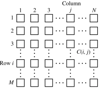
A standard CNN or Continuous Time CNN (CTCNN) architecture [13] consists of an M × N rectangular array of cells C(i,j) with Cartesian coordinates (i, j), i = 1, 2, ..., M, j = 1, 2, ..., N (Fig. 2.1).
Figure 2.1: Architecture of a CNN In some applications M may not be equal to N .
The sphere of influence [13], Sr(i, j), of the radius r of cell C(i, j) is defined to be the
set of all the neighborhood cells satisfying the following property
Sr(i, j) = {C(k, l)| max
1≤k≤M,1≤l≤N {|k − i|, |l − j|} ≤ r} (2.1)
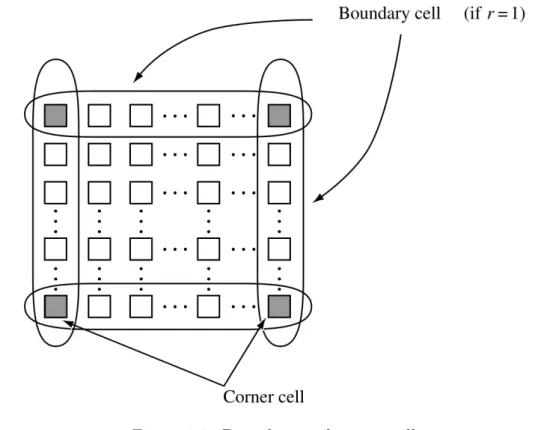
A cell C(i, j) is called a regular cell [13] with respect to Sr(i, j) if and only if all
neighborhood cells C(k, l) ∈ Sr(i, j) exist. Otherwise, C(i, j) is called a boundary cell (Fig.
2.2).
Figure 2.2: Boundary and corner cells
There are M × N rectangular array of cells in a CNN, hence it is called a M × N CTCNN. A single cell C(i, j) resides at location (i, j), i = 1, 2, ..., M, j = 1, 2, ..., N .
Properties for each cell C(i, j) can be presented as: State Equation . xij = −xij + X C(k,l)∈Sr(i,j) A(i, j; k, l)ykl+ X C(k,l)∈Sr(i,j) B(i, j; k, l)ukl +zij (2.2)
where xij ∈ R is called state, ykl ∈ R output, ukl ∈ R input, and zij ∈ R
thresh-old. A(i, j; k, l) and B(i, j; k, l) are called feedback and control operators respectively whose functions will be explained later.
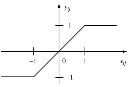
Output Equation yij = f (xij) = 1 2|xij + 1| − 1 2|xij − 1| (2.3)
where f (xij) is called the output function which is a piecewise linear function (Fig. 2.3) but
nonlinear overall. f (xi,j) has the property to saturate to +1 and -1 for input values over
+1 and below -1 respectively.
Figure 2.3: Plot of f (xi,j)
Boundary Conditions
The boundary conditions specify ykl and ukl that lie outside of the M × N array but
belong to Sr(i, j) of edge cells.
Initial State
xij(0), i = 1, ..., M, j = 1, ..., N (2.4)
where xij(0) defines the initial state. Initial state is defined according to the application
A block diagram of a CNN [14] can be seen in Fig. 2.4 which is a graphical represen-tation of the state equation Eq. (2.2). In this diagram f is the activation function, in other words the output y.
Figure 2.4: Block diagram of a CNN
Dimensions of the CNN is usually chosen to match the dimensions of the input image M × N and input uklis equal to the normalized gray-scale pixel intensity when used in image
processing applications. Normalization is performed in the range −1 ≤ ukl ≤ +1 where −1
and +1 corresponds to white and black respectively. Also the normalized image no longer consists of integer pixel intensities but floating point values to ensure no loss of generality. For video applications, ukl is a function of time where other variables can be specified as
images.
The Discrete Time Cellular Neural Network (DTCNN) [15] is a discrete-time, nonlin-ear, first-order dynamical system consisting of M identical cells on a 1D or 2D cell grid. M input ports are placed on an input grid with identical dimensions. Usually input is an image and output is a manipulation of the image.
DTCNNs differ from a CTCNN in the following aspects: State Equation xij(n + 1) = X C(k,l)∈Sr(i,j) A(i, j; k, l)ykl(n) + X C(k,l)∈Sr(i,j) B(i, j; k, l)ukl +zij (2.5) Output Equation yij(n) = f (xij(n)) (2.6)
where f (xij) = sgn(xij) = 1 : xij ≥ 0, 0 : xij < 0. (2.7)
and the initial state is xij(0). uij, yij(n), xij(n), and zij are the input signal, the output
signal, the state, and the bias of cell (i, j) at time-step n. Insertion of a nonnegative integer time-step n makes a DTCNN function differently from a CTCNN where a standard CNN would require an ordinary differential equation to be solved to evaluate ˙xij. Although signum
function is defined as the output function for a DTCNN, piecewise linear output function Eq. (2.3) of CTCNN is used for a DTCNN in this study.
2.1 Dynamics of DTCNNs
A DTCNN can be modeled only with its initial state x(0), bias z, and cloning templates A and B. zij can be chosen as one single value for all cells. A DTCNN is ready to do
processing after these values are defined.
Processing of a DTCNN works in an iterative manner. Following steps are performed for each iteration:
1- Output y(1) is evaluated using the initial state x(0) by the piecewise linear function Eq. (2.3).
y(0) = 1
2|x(0) + 1| − 1
2|x(0) − 1| (2.8)
2- Next state x(1) is calculated by using the state equation (2.5).
To find the next iterative value of x(n), feedback operator A is convolved with output y(n), control operator B is convolved with input u and the bias z is added to the resulting sum of the two convolutions. Here A and B may also be called convolutional filters.
If the output y has not converged to +1 or −1, the next iteration takes place starting at step 1 again. The end of processing is determined by the convergence of output y. If every element of y converges to the same value after 2 consequent iterations then the processing is complete. In other words,
yij(n + 1) = yij(n), ∀yij ∈ {+1, −1}. (2.10)
The convergence of y(n) can also be determined from the absolute difference of 2 con-sequent states (x(n), x(n − 1)) values. If the absolute difference is below a defined maximum error emax then no further iterations are necessary. That is,
1 M × N M X i=1 N X j=1 |xij(n) − xij(n − 1)| !
≤ emax ⇒ y(n) = y(∞). (2.11)
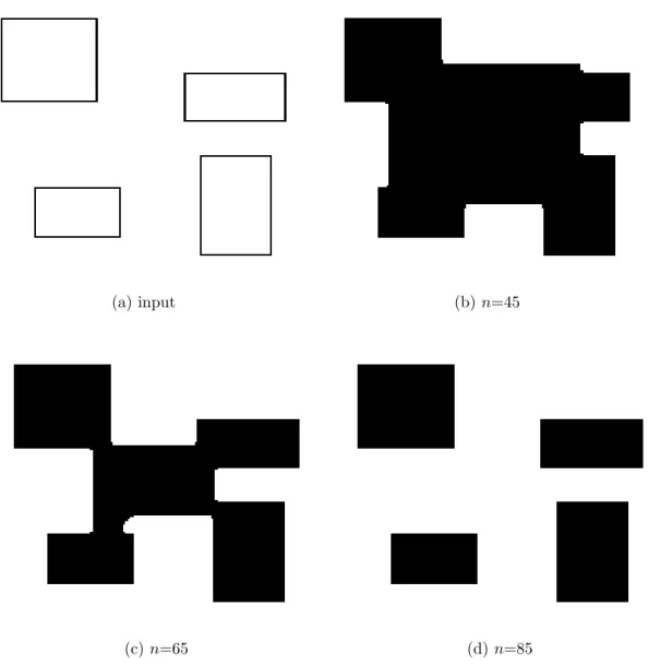
As an example, an object filling application performed with a DTCNN is illustrated in Fig. 2.5. In this example the initial value of each state variable xij is initialized to one which
corresponds to a black pixel. Input and output of the DTCNN after various iterations steps are shown. Output converges after 85 iterations so no further iterations are necessary.
(a) input (b) n=45
(c) n=65 (d) n=85
Figure 2.5: (a) Input image and output after (b)n=45, (c)n=65, (d)n=85 iterations
2.2 Stability of CNN
Stability of a DTCNN determines the output characteristics. Stability depends on two conditions [16]. The corresponding two conditions are,
1- Space Invariance Property: Space invariance property is defined as
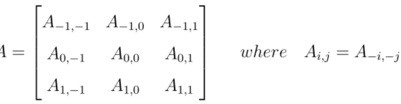
It can also be realized as the symmetry with regards to the center element as depicted in Fig. 2.6. Center element corresponds to element A0,0 of the matrix in Fig. 2.6. A 3 × 3
(r = 1) size feedback operator A has the space invariance property if resembles the matrix in Fig. 2.6. A = A−1,−1 A−1,0 A−1,1 A0,−1 A0,0 A0,1 A1,−1 A1,0 A1,1
where Ai,j = A−i,−j
Figure 2.6: A symmetric feedback operator A
A DTCNN is completely stable if it has space invariance property. Completely stable means the output of the DTCNN will converge to a fixed number after uncertain number of iterations. ’Uncertain’ means number of iterations can be calculated or predicted.
2- Binary Output Property: If the self feedback coefficient of feedback operator is bigger than or equal to 1, then the CNN has the binary output property.
A0,0 ≥ 1 (2.13)
If a DTCNN is completely stable and has the binary output property that means its output y will converge to {+1, −1}. Self feedback coefficient is the matrix element A0,0 in
Fig. 2.6.
When these two conditions are met, outputs of DTCNN are guaranteed to converge to +1 or −1 after the input is processed. Stability isn’t any way related to how many iterations it will take DTCNN to converge though.
2.3 Template Learning of CNNs
Learning is the action of training when neural networks are considered in general. After a neural network is trained to do some task, input is fed into the neural network and the output is as close as to the desired if not the desired output itself. That makes neural networks very suitable for many hard to theorize tasks. There are two ways of training, supervised or unsupervised. When supervised training is performed, the system parameters of the neural network is adjusted according to an error function which is a function of desired output and it is trained to give outputs close the desired outputs by the use of a training algorithm.
Various training algorithms have been proposed since the CNNs have surfaced. Each of them have their advantages and disadvantages. Choosing a suitable algorithm for both the type of CNN and type of processed data is important. Type of the training algorithm may also effect the performance.
A proposed method to train a CNN is to use a Multilayer Perceptron (MLP) [17]. Here dynamic behavior of CNN when converged to a fixed-point is reproduced with a MLP using the adequate number of input, hidden and output layers. Then the similarities and parameter relations between the CNN and MLP are used to find the template coefficients. Modeling a M × N CNN with a MLP makes the MLP more complex when M and N is large as the complexity of MLP increases more than the complexity of CNN.
Recurrent Perception Learning Algorithm (RPLA) [18] is a supervised algorithm for obtaining the template coefficients in completely stable CNNs. RPLA resembles the per-ceptron learning algorithm for neural networks, hence the name RPLA. The RPLA can be described as the following set of rules: (i) increase each feedback template coefficient which defines the connection to a mismatching cell from its neighbor whose steady-state output is same with the mismatching cell’s desired output. On the contrary, decrease each feedback template coefficient which defines the connection to a mismatching cell from its neighbor whose steady-state is different from the mismatching cell’s desired output. (ii) Change the
input template coefficients according to the rule stated in (i) by only replacing the word of neighbor with input. (iii) Retain the template coefficients unchanged if the actual outputs match the desired outputs. RPLA algorithm suffers from the local minimum problem like its MLP version.
Genetic algorithms may also be used to train a CNN [19]. This method uses a genetic optimization algorithm to derive template coefficients. The difference between the settled output and the desired output is used to evaluate the CNN templates. Minimizing this is achieved by changing the template coefficients. A cost function is used to adjust the change in the template coefficients. A learning algorithm may stuck in a local minimum while training. This may end the training process with undesired template coefficients where better coefficients exist. The cost function used in genetic algorithms has the superiority that it can find the global minimum in noisy and discontinuous environments. This makes genetic algorithms a better alternative to mathematical algorithms.
A new learning algorithm is proposed on this thesis making use of Bayesian learning theory. It is a probabilistic learning algorithm involving prior and likelihood probability densities to estimate the template coefficients. In this probabilistic model, the learning problem is turned into an estimation problem and template coefficients are estimated by Bayesian learning.
Chapter 3
BAYESIAN LEARNING
Bayesian learning is the process of updating the probability estimate for a hypothesis as additional prior knowledge is gathered and it is an important probabilistic technique used in various disciplines. Bayesian learning is used in image processing [20], machine learning [21], mathematical statistics [22], engineering [23], philosophy [24], medicine [25], law [26] etc...
The Bayesian framework [27] is distinguished by its use of probability to express all forms of uncertainty. Bayesian learning results in a probability distribution of system pa-rameters that yields how likely the various parameter values are. Before applying Bayesian learning, a prior distribution in behalf of prior information must be defined. After obser-vations are made, this prior distribution becomes a posterior distribution in conjunction with Bayes theorem Eq. (3.3). The resulting posterior distribution contains information from both the observation of parameters (likelihood) and the background knowledge about the parameters (prior). Introducing the prior information here, transforms the likelihood function into a probability distribution thus making use of probability theory possible.
Computational difficulties arise when the resulting posterior density function is diffi-cult or impossible to sample with procedural methods. That is where the use of Markov chain Monte Carlo (MCMC) methods come in for the rescue. MCMC methods are used to overcome the computational problems in Bayesian learning. Whereas a linear system has a posterior distribution that has no computational burden.
3.1 Bayes Theorem
Bayes theorem is important in probability in a way that it expresses how a subjective degree of belief should rationally change to account for evidence. In other words it predicts how much the outcome of some event is effected with the prior knowledge about the random
variables associated with that event.
Bayes theorem can easily be derived using the definition of conditional probability [28],
P (A|B) = P (A ∩ B)
P (B) , P (B) 6= 0 (3.1)
Conditional probability gives the probability of event A in case event B occurred. The inverse must also hold true,
P (B|A) = P (A ∩ B)
P (A) , P (A) 6= 0 (3.2)
Inserting P (A ∩ B) of Eq. (3.1) into Eq. (3.2) gives the Bayes theorem in its pure form,
P (A|B) = P (B|A)P (A)
P (B) , P (B) 6= 0 (3.3)
where,
P (A|B) is the posterior probability, P (B|A) is the likelihood,
P (A) is the prior probability of A,
P (B) is the prior probability of B or marginal likelihood.
In many applications P (B) is fixed and the interest is in the change of P (A) so in these cases where P (B) is fixed, posterior is proportional to likelihood times prior,
3.2 Maximum A Posteriori (MAP) Estimation
Maximum a posteriori estimation uses the posterior distribution to obtain an estimate of an unobserved quantity by using empirical data. MAP resembles the maximum likelihood (ML) method specializing in a way that it includes the prior knowledge in the estimation process. MAP gives the best estimation results amongst other probabilistic methods purely because of the fact that it includes the prior knowledge.
ML estimation of parameter θ is defined as,
ˆ
θM L = argmax θ
p(y|θ) (3.5)
where ˆθ is the estimation of θ. No prior information is involved in the ML estimation which is a consequence of its design. If a prior distribution can be defined for θ then MAP estimation will give the best estimation results possible for a probabilistic theory. MAP estimation of parameter θ is defined as,
ˆ
θM AP = argmax θ
p(θ|y) (3.6)
and using the Bayes theorem it is transformed into,
ˆ
θM AP = argmax θ
p(y|θ)p(θ)
p(y) (3.7)
and after expanding the denominator, ˆθ can finally be denoted as,
ˆ θM AP = argmax θ p(y|θ)p(θ) R θ∈Θp(y|θ)p(θ)dθ (3.8)
The integral in the denominator gets quite messy for multi-dimensional and nonlinear estimation problems but fortunately it is also independent of θ which makes it vanish in the
derivation step. MCMC methods are used to reduce the computational complexity for these problems.
A simple way to maximize θ is to take the derivative of Eq. (3.7) with respect to θ and equating the result to zero. To facilitate computations, logarithm of Eq. (3.7) can be used in the derivation. This will not change the result of the estimation regarding the fact that the derivative with respect to x of the logarithm of a function of x is,
d ln f (x)
dx =
f0(x)
f (x) (3.9)
The denominator will cancel out when equalized to zero. So logarithm of MAP estimation for θ, ˆ θM AP = argmax θ lnp(y|θ)p(θ) p(y) (3.10) = argmax θ [ln p(y|θ) + ln p(θ) − ln p(y)] becomes, d ln [p(y|θ)p(θ)] dθ = 0 (3.11)
after derived with respect to θ and equalized to zero.
A simple example of a MAP estimation is estimating the aim for a set of noisy samples. The equation of the system is,
y[n] = θx[n] + ω[n] n = 0, 1, ..., N − 1 (3.12)
or in vector form,
where y[n] is the output sequence, x[n] is the input sequence, w[n] is the noise, and θ is the aim parameter to be estimated. θ has a prior distribution of a Gaussian PDF with mean µθ
and variance σθ2. ω also has a Gaussian PDF with mean µωand variance σω2. Both means (µθ,
µω) are assumed to be zero for this simple example to make things easier. Likelihood p(y|θ)
is a Gaussian distribution N (θx, σ2ω) as noise ω has zero mean and θx has zero variance. So
y|θ ∼ N (θx, σω2I) (3.14)
And accompanying PDFs for likelihood p(y|θ) and prior p(θ) are,
p(y|θ) = pω(y − θx) = 1 p(2πσ2 ω)N e −(y − θx) >(y − θx) 2σ2 ω p(θ) = 1 p2πσ2 θ e − θ 2 2σ2 θ (3.15)
Taking these into account and using Eq. (3.10), ˆθ can be written as,
ˆ θM AP = argmax θ ln 1 p(2πσ2 ω)N e −(y − θx) >(y − θx) 2σ2 ω 1 p2πσ2 θ e − θ 2 2σ2 θ p(y) (3.16)
Or by expanding the terms inside the logarithm,
ˆ θM AP = argmax θ ln 1 p(2πσ2 ω)N e −(y − θx) >(y − θx) 2σ2 ω + ln 1 p2πσ2 θ e − θ 2 2σ2 θ − ln p(y) (3.17)
Since y(0), y(1), ..., y(N − 1) are independent of each other, p(y) can be written as,
p(y) = p(y(0), y(1), ..., y(N − 1)) =
N −1
Y
n=0
For the same reason p(y|θ) can also be written as, p(y|θ) = N −1 Y n=0 p(y(n)|θ) (3.19)
And when reintroduced with the PDFs of each sample, ln p(y|θ) becomes,
ln p(y|θ) = ln N −1 Y n=0 1 p2πσ2 w e −(y(n) − θx(n)) 2 2σ2 ω (3.20)
By the definition of logarithm, ln p(y)|θ) can be written as,
ln p(y|θ) = N −1 X n=0 ln 1 p2πσ2 w e −(y(n) − θx(n)) 2 2σ2 ω (3.21)
By inserting the final form of ln p(y|θ) and expanding the products inside the logarithms, ˆθ can finally be written as,
ˆ θM AP = argmax θ N −1 X n=0 ln e −(y(n) − θx(n)) 2 2σ2 ω + ln e − θ 2 2σ2 θ (3.22) + N ln 1 p2πσ2 ω + ln 1 p2πσ2 θ − ln p(y) #
The last 3 terms are independent of θ and will vanish in the derivation. Taking the derivative of ˆθ with respect to θ and equating the result to zero gives,
ˆ θM AP = 1 σ2 ω N −1 P n=0 x(n)y(n) 1 σ2 θ + 1 σ2 ω N −1 P n=0 x2(n) = x >.y σ2 ω σ2 θ + x>.x (3.23)
which is the analytical estimation of θ.
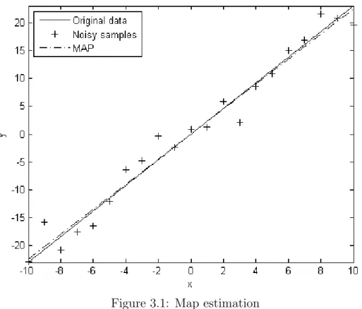
A numeric example to comment on the outcome of the MAP estimation is illustrated below. θ is chosen to be 2.3 for this example, that is,
y = θx + ω, θ = 2.3 (3.24)
where ω is additive noise with a Gaussian distribution N (0, 4). Prior distribution is also chosen to be a Gaussian distribution N (1, 2). Sample pairs of x and y are populated using Eq. (3.24) and then Eq. (3.23) is used to calculate ˆθ which is evaluated as ˆθ = 2.24 against the original value of θ = 2.3. Results are plotted in Fig. 3.1.
Figure 3.1: Map estimation
For estimation problems where the posterior PDF cannot be derived, Metropolis-Hastings algorithm is one way to generate samples from the posterior PDF and take the average of these samples to make an estimation.
3.3 Markov Chain Monte Carlo
In statistics, Markov Chain Monte Carlo (MCMC) methods are a class of algorithms for sampling from the probability distributions based on constructing a Markov chain that has the desired distribution as its equilibrium distribution [29]. Often after a large amount of steps, the state of the chain converges to the desired distribution which can then be used as a sample. As the number of steps are increased the quality of the sample improves as a function of it.
A Markov chain [30] is a mathematical system that undergoes transitions from one state to another, between a finite or countable number of possible states. It is a stochastic process. The next state of a Markov process does not depend on any previous states but only on the current state, giving it the memoryless property. This is also called the Markov property.
Considering experiments [31] which the outcomes of these experiments are equally likely and independent of each other, knowledge of the previous outcomes for these experiments have no effect on the predictions for the outcomes of the proceeding experiments. Sequence of these experiments may be used to construct a tree of for example n experiments and this tree can be used to answer probability questions about these experiments.
To specify a Markov chain, a set of states S = {s1, s2, ..., sr} must be designated. A
process begins at one of the states and moves successively to another state from its current state in each step. The probability pij of moving from state si to state sj is independent
from the previous state of the process.
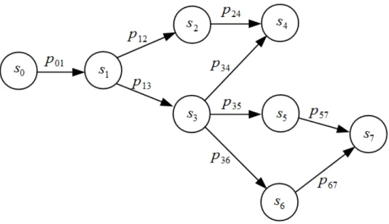
The probabilities pij are called transition probabilities as shown in Fig. 3.2. The process
may stay at its current state without moving to any other state with the probability pii. An
Figure 3.2: A simple Markov chain
A Markov chain can also be presented with the transition matrix. The elements of a transition matrix represent the transition probabilities between the intersections. A transi-tion matrix P for a set of N states is of N × N size and given below,
P = p0,0 p0,1 · · · p0,N p1,0 p1,1 · · · p1,N .. . ... . .. ... pN,0 pN,1 · · · pN,N (3.25)
The matrix element pij is the transition probability from state i to state j. Transition
matrix is not required to be symmetrical as state transitions may be one directional or have different probabilities for pij and pji.
Convergence of a Markov chain may be defined as the resemblance of the histogram of the samples to the distribution used to generate the samples. Here the probability of the states corresponds to the points on the PDF acquired from the histogram of the samples.
Construction of a Markov chain satisfying the desired properties is usually not so difficult. The challenge lies in the determination of the number of steps that are needed to converge to the desired distribution within an acceptable error. A good chain which has rapid mixing, will resemble the desired distribution quickly starting from an arbitrary position. Rapid mixing is defined under Markov chain mixing time.
Normal usage of MCMC sampling doesn’t go far from approximating the desired dis-tribution considering the unwanted effect regarding the starting postion. Better and more sophisticated MCMC-based methods, i.e. coupling from the past can generate exact samples of the desired distribution. These methods require more computational burden and indefinite running time.
These algorithms are commonly applied to evaluate multi-dimensional integrals numer-ically. These methods introduce the walker concept where a walker moves around randomly to find a place with reasonably high contribution to the integral. Random walk methods can be considered as a random simulation or Monte Carlo method. Nonetheless, random samples of the integrand achieved by the random walk of the walker in a conventional Monte Carlo integration are statistically independent but the samples achieved by MCMC are correlated. A Markov chain is to have the integrand as its desired distribution which is often not so hard to accomplish.
Markov chain Monte Carlo methods are widely used in Bayesian statistics, computa-tional physics, computacomputa-tional biology and computacomputa-tional linguistics where multi-dimensional integrals often are the case.
Most MCMC methods takes relatively small steps to move around the desired distri-bution and with no intention to take the steps in the same direction. Apart from being easy to implement, these methods may consume relatively long times for the walker to explore all of the sample space and also may revisit the space already explored. Some examples to these methods are Metropolis-Hastings algorithm (the one chosen for this study), Gibbs sampling, Slice sampling, and Multiple-try Metropolis.
More sophisticated algorithms implement a method to prevent the walker from walking back to the already explored parts of the space. Although these methods are harder to implement, they may provide faster convergence. Some of these algorithms are Successive over-relaxation, Hybrid Monte Carlo, some variations of slice sampling, Langevin MCMC, and other methods that rely on the gradient of the log posterior.
There are other MCMC methods that change the dimensionality of the space. To name one, the reversible-jump method is a variant of Metropolis-Hastings which makes use of the proposals to change the dimensionality of the space. These methods find usage in statistical physics applications where a grand canonical ensemble distribution needs to be used.
3.4 Metropolis-Hastings Method
Metropolis-Hastings [12] [32] method is one of the various Monte Carlo Markov Chain (MCMC) methods that is useful for obtaining a sequence of random samples from a prob-ability distribution. It is used when direct sampling is either difficult or impossible. The distribution is approximated with this method and the histogram generated will trace the actual distribution. Metropolis-Hastings method can also be used for sampling from multi-dimensional distributions which is the case for this thesis. This method is chosen for its simplicity and effectiveness.
The only requirements for Metropolis-Hastings method to work are the availability of a function f (x) that is proportional to the probability density of the distribution (PDF) and the value of f (x) can be calculated. The advantage to this algorithm is that it can work with proportional functions to the PDF rather than requiring the PDF itself.
The idea behind Metropolis-Hastings method is that after a sequence of samples pro-duced in an increasing number, the distribution of the generated samples will converge to the PDF itself. When the samples are produced iteratively, the next sample depends on the current sample thus making these sequence of samples into a Markov chain. After the next sample candidate is generated, the sample itself is accepted for the next in sequence with a
probability that is decided by comparing the likelihoods of the current and candidate sample values with respect to the PDF.
Metropolis algorithm [11], a special case for Metropolis-Hastings method has two stages to succeed, presented below:
1- Initialization: An arbitrary point x0 is chosen for the first sample. This decision
of an arbitrary point may effect the convergence of the resulting sample distribution as it may not converge to the desired distribution in a practical number of samples if it’s badly chosen. An arbitrary probability density Q(x|y) is chosen to generate the next sample candidate x around the previous sample y. Metropolis algorithm requires Q to be symmetric Q(x|y) = Q(y|x) thus it’s chosen to be a Gaussian centered at y most of the time. Q is called proposal density or jumping distribution.
2- Iteration:
• Next sample candidate x0 is generated from the distribution Q(x0|x).
• The acceptance ratio α is calculated according to the ratio f (x0)/f (x). Here f (x)
may be the desired PDF if it’s available.
• The value of α is used to decide whether to accept or reject the sample candidate x0.
If α ≥ 1, the candidate is directly accepted else the candidate is accepted with α probability. That is if α is greater than a uniformly distributed number α0 then it is accepted and rejected otherwise. If the candidate is rejected, current sample is put next in sequence.
The iteration step is repeated until there are enough samples to approximate the desired distribution. The algorithm basically moves in the sample space, accepting the more probable samples and mostly rejecting the less probable samples. By the use of this algorithm low density regions of f (x) are visited occasionally and samples are mostly generated from high density regions of f (x).
There are a couple of disadvantages to Metropolis-Hastings method. The generated samples are correlated resulting from the proposal density function Q(x|y) depending on the previous sample. This is especially true for consequent samples although the overall process approximate the desired PDF. To overcome this correlation problem, every nth sample can be
taken from the resulting sequence. n depends on the autocorrelation of consequent samples. Autocorrelation can be reduced by increasing the variance of the proposal density in which case the samples will be further apart but this also decreases the probability that the sample candidate will be accepted. These parameters must be chosen carefully for a reasonable estimate of the desired distribution.
Another disadvantage of the Metropolis-Hastings method is the initial samples gener-ated around the initial point x0 may not follow the desired distribution if the x0 is chosen
in a low density region. One may overcome this problem by discarding the first necessary number of samples.
Compared to other sampling methods, Metropolis-Hastings method does not suffer from the curse of dimensionality where the probability of rejecting the sample candidates increases exponentially as a function of dimensions, to the point where other methods suffer. And usually it is the only logical method to sample from a desired distribution.
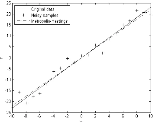
To compare the results of the algorithm, numeric example of MAP estimation is used again, this time with Metropolis-Hastings method. Noisy samples are again generated using,
y = θx + ω, θ = 2.3 (3.26)
where ω has a Gaussian distribution N (0, 4). Prior distribution is also chosen to be a Gaussian distribution N (1, 2). Sample pairs of x and y are populated using Eq. (3.26) and then Metropolis-Hastings algorithm is used to calculate ˆθ which is evaluated as ˆθ = 2.19 against the original value of θ = 2.3. Results are plotted in Fig. 3.3.
As can be seen from Fig. 3.3, Metropolis-Hastings algorithm can give a good estimate for θ. Same result can also be used to compare it with MAP algorithm. It can be con-cluded that both algorithms give similar results making Metropolis-Hastings algorithm an alternative to MAP algorithm where the PDF of the target distribution cannot be derived.
Chapter 4
TRAINING DTCNNs USING BAYESIAN LEARNING
4.1 System Model
Before a DTCNN is ready to process the input data, it must be trained. Training step tells the DTCNN how to act on the input data. The training step is crucial to setup the DTCNN. Before starting the training step, DTCNN must be initialized with the initial feedback (A), control (B) operators and the bias (z) value. The initial value of feedback operator is chosen according to the stability criteria mentioned in Sec. 2.2. Considering this, there are only 5 different coefficients for a feedback operator of size 3 × 3 satisfying the space invariance property, A = b c d e a e d c b (4.1)
Satisfying the space invariance property also for the control operator B makes a total of 11 coefficients to start the training with, including the bias coefficient. B is also in the same form as A, B = g h i j f j i h g (4.2)
The column vector θ of the estimated coefficients can be constructed from the coeffi-cients of A and B and the bias as follows,
where k represents the bias z. The placement of the coefficients are arranged according to the implemented software.
Main equation for the system model then becomes,
y = f∞(x, u, θ) + ω (4.4)
where x is the state, u is the input, y is the desired output, ω is the noise, and f∞ is
the processing function of the CNN till the CNN converges, denoted by the ∞ subscript. There is no analytical representation for the f∞ as the CNN design is recursive so f∞ is
considered as the output for the CNN after certain number of iterations. Although the space invariance property guarantees the CNN to converge, it doesn’t guarantee the convergence in a reasonable number of iterations so for practical reasons number of iterations required to conclude the output is usually limited according to the application.
The state variable x is an intermediate variable which is affiliated with the output y. In fact y is a function of x and only y is of importance in the output of CNN other than the initial value of x. Because of this, x variable will not be included in the CNN output function f∞ from now on.
Additive noise ω is added to transform the training step into an estimation problem which makes usage of the MAP estimation possible. After the system is transformed then the underlying probabilistic tools can be used to estimate the network parameters. The additive noise has a Gaussian PDF with variance σ2ω and its mean µω is assumed to be zero
for this study.
For discrete samples, the corresponding parameters are indexed with n,
y[n] = f∞[n](u, θ) + ω[n] , n = 0, 1, ..., N − 1 (4.5)
where each u[n] and y[n] corresponds to a pixel of the input image and its output in the output image respectively as images are considered as inputs and outputs. The superscript
[n] is used to index the nth output of function f∞. Here inputs u are known. Using the
vector notation Eq. (4.5) can be restated as,
y = f∞(u, θ) + ω (4.6)
Likelihood p(y|θ) is a Gaussian distribution with mean f∞(u, θ) and variance σω2 since
noise ω has zero mean and variance σ2ω,
y|θ ∼ N (f∞(u, θ), σω2I) (4.7)
As each p(y(n)|θ) is independent of each other, p(y|θ) can be written as,
p(y|θ) = p(y(0)|θ)p(y(1)|θ)...p(y(N − 1)|θ) (4.8)
and the resulting p(y|θ) becomes,
p(y|θ) = pω(y − f∞) = N −1 Y n=0 1 p2πσ2 ω e −(y[n] − f [n] ∞(u, θ))2 2σ2 ω (4.9)
Prior distribution of θ is also assumed to be Gaussian. The means of network param-eters θ1, θ2, ..., θ11 is the column vector,
µθ = [µθ1, µθ2, ..., µθ11] >
and variances of network parameters σ12, σ22, ..., σ112 resides in the covariance matrix, Σθ = σ2 1 0 · · · 0 0 σ22 · · · 0 .. . ... . .. ... 0 0 · · · σ112 (4.11)
where Σθ represents the covariance matrix. Network parameters θ1, θ2, ..., θ11 are assumed
to be uncorrelated for this study. Because of this, cross correlation terms are zero. Prior PDF can be written using the means vector and covariance matrix in matrix form,
p(θ) = 1 p(2π)11|Σ θ| e− (θ − µθ)>Σ−1θ (θ − µθ) 2 (4.12)
where |Σθ| is the determinant of the covariance matrix.
Combining both the likelihood and prior PDFs gives the posterior PDF for the overall system, p(θ|y) = N −1 Y n=0 1 p2πσ2 ω e −(y[n] − f∞[n](u, θ))2 2σ2 ω (4.13) × 1 p(2π)11|Σ θ| e− (θ − µθ)>Σ−1θ (θ − µθ) 2
As stated before the requirement for MAP estimation is,
ˆ
θM AP = argmax θ
p(θ|y) (4.14)
Unfortunately Eq. (4.13) is not derivable because of the piece wise linear function used in the CNN. To overcome this problem Metropolis-Hastings method is implemented as
an alternative to the analytical method. To achieve the estimation of network parameters, Metropolis-Hastings method is used to generate samples from Eq. (4.13).
4.2 Metropolis-Hastings Implementation
As stated before Metropolis-Hastings method generates samples from the given dis-tribution by using an algorithm which basically tries to find a better sample candidate by comparing the probability of the new sample against the one comes before it. A better explanation would be to demonstrate the algorithm.
Before the samples are generated, an initial point must be chosen. The closer this initial point is to the optimal value of the network coefficient, the faster the sample sequence will converge to the desired distribution. This point may be predicted according to the prior information,
θ(0) = [θ0(0), θ1(0), ..., θ11(0)] >
(4.15)
where θ(0) is the vector of initial points for each network coefficient.
After the initial points are determined, a new sample vector θnewis generated according
to the proposal density. Proposal density must be a symmetric distribution like the Gaussian distribution which is also chosen to be the proposal density for the Metropolis-Hastings algorithm implemented in this study. For the new sample vector to take its place in the sample sequence, it must be trialled using the posterior distribution of Eq. (4.13). To manage this, the following proportion which is denoted by α, is evaluated,
α = p(θnew|y)
p(θ(k − 1)|y) (4.16)
where p(θnew|y) is the posterior distribution evaluated with the new sample vector and
constants in the nominator and denominator of Eq. (4.13) which doesn’t involve any variables cancel out in the proportion of Eq. (4.16) and the products of p(y|θ) can be written as a sum in the exponent. Then the resulting equation for α becomes,
α = e
− N −1
P
n=0
(y[n] − f∞[n](u, θnew))2
2σ2 ω .e −(θnew− µθ) >Σ−1 θ (θnew− µθ) 2 e − N −1 P n=0 (y[n] − f∞[n](u, θ(k − 1)))2 2σ2 ω .e −(θ(k − 1) − µθ) >Σ−1 θ (θ(k − 1) − µθ) 2 (4.17)
If α ≥ 1 then the new sample vector is inserted directly into the sample sequence. If α < 1 then it is accepted with α probability. To manage this, a random number denoted by α0 is generated from a uniform distribution of U (0, 1) and then α is compared with α0. In the case where α ≥ α0, the new sample vector is inserted into the sample sequence. Otherwise the preceding sample vector is inserted into the sample sequence. The acceptance of the new sample vector is summarized below,
α ≥ 1 ⇒ θ(k) = θnew (4.18)
α < 1 & α ≥ α0 ⇒ θ(k) = θnew
α < 1 & α < α0 ⇒ θ(k) = θ(k − 1)
After the new sample candidate or the previous one is inserted into the sample sequence, the loop starts again by producing a new sample vector by using the proposal density and continues till the intended number of samples are generated. Then the resulting sample sequences for each parameter are averaged to estimate the parameter itself.
Samples sequences of network coefficients are in the following form, θ(0) = [θ1(0), θ2(0), ..., θ11(0)] > (4.19) θ(1) = [θ1(1), θ2(1), ..., θ11(1)] > .. . = ... θ(K − 1) = [θ1(K − 1), θ2(K − 1), ..., θ11(K − 1)] >
where K is the total number of samples generated. To calculate the mean of each coefficient, the resulting summation of each sample is divided by K,
E[θ|y] = 1 K K−1 X k=0 θ(k) (4.20) = θ(0) + θ(1) + ... + θ(K − 1) K
where E[θ|y] is the expected value of θ with respect to y, namely the average of θ|y. The resulting estimation of θ|y in vector form is,
ˆ
θ =hˆb, ˆc, ˆd, ˆe, ˆa, ˆg, ˆh,ˆi, ˆj, ˆf , ˆki
>
(4.21)
and these coefficients are then used for testing.
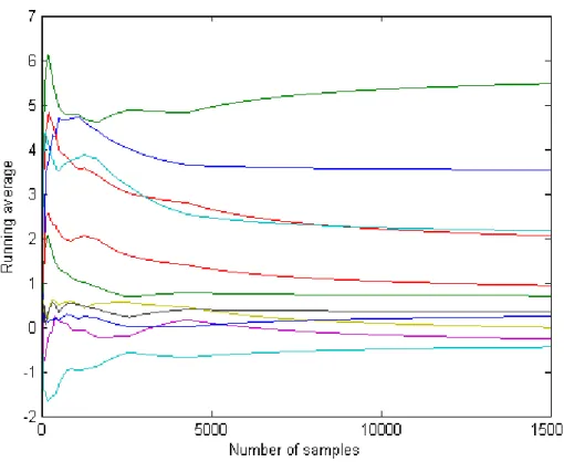
Convergence of the network coefficients for a single run of the implemented software can be seen in Fig. 4.1. The term running average is the calculated average (mean) of the present samples so far each time a new sample is generated. Then these running averages are plotted versus the number of samples. As can be seen from Fig. 4.1, network coefficients converge to their intended values after certain number of iterations.
Figure 4.1: Convergence of network coefficients
Software used for this study is implemented in C++ programming language using various open source tools [33][34][35][36].
Chapter 5 RESULTS
Implemented DTCNN is trained for an edge detection application to be used in image processing. In this application edges in the input are detected by highlighting the edges. The input and desired output images in Fig. 5.1 are used for training.
(a) input image u (b) desired output y
Figure 5.1: Input (a) and desired output (b) of edge detection application
In the training step Eq. (2.3) and Eq. (2.5) are used to evaluate f∞(u, θ(k)) for
each sample. During the training step, number of iterations for each sample is limited to 100 meaning next iteration is not performed if the network hasn’t converged after 100 iterations. This limit can be higher with more computer power but for practical reasons 100 is a reasonable number.
State variable is the same as the input image for this edge detection application. Final output is gathered from the final iteration of the state variable. When the processing starts again after each sampling, state variable is initialized to its initial state which is the input image itself for this application.
After 10000 samples for each parameter, ˆθ is evaluated as (shown with only 2 digits of precision),
ˆ
θ = [−0.49, 0.41, 0.27, −0.39, 6.53, −2.82, 0.45, −3.84, 2.47, 0.41, −2.44]> (5.1)
Resulting feedback and control matrices and bias are,
A = −0.4974 0.4150 0.2714 −0.3985 6.5357 −0.3985 0.2714 0.4150 −0.4974 (5.2) B = −2.8228 0.4582 −3.8480 2.4702 0.4180 2.4702 −3.8480 0.4582 −2.8228 (5.3) z = −2.4452 (5.4)
Test input image is processed using these coefficients with the help of Eq. (2.3) and Eq. (2.5). Actual output of the system is defined as,
y = f∞(u, ˆθ) (5.5)
(a) input (b) actual output
Figure 5.2: Input (a) and actual output (b) of edge detection application
Another implementation is the object filling algorithm. Empty objects in the input image are filled by using this algorithm in image processing. To train the system, the input and desired output images in Fig. 5.3 are used.
(a) input image u (b) desired output y
In the training step Eq. (2.3) and Eq. (2.5) are used to evaluate f∞(u, θ(k)) for each
sample. During the training step, number of iterations for each sample is limited to 250 meaning next iteration is not performed if the network hasn’t converged after 250 iterations. This limit heavily depends on the size of the input image but for the input image used in this application 250 is a reasonable number.
State variable is initialized to ones for this object filling application. It is initialized to ones again after each sampling.
After 10000 samples for each parameter, ˆθ is evaluated as (shown with only 2 digits of precision),
ˆ
θ = [1.44, 1.74, 1.57, 2.31, 2.27, 0.13, 2.90, 0.57, 2.29, 3.76, 2.22]> (5.6)
Resulting feedback and control matrices and bias are,
A = 1.4454 1.7490 1.5799 2.3162 2.2744 2.3162 1.5799 1.7490 1.4454 (5.7) B = 0.1335 2.9051 0.5742 2.2910 3.7654 2.2910 0.5742 2.9051 0.1335 (5.8) z = 2.2238 (5.9)
Test input image is processed using these coefficients with the help of Eq. (2.3) and Eq. (2.5). Actual output of the system is defined as,
y = f∞(u, ˆθ) (5.10)
Objects in test input image are filled after 321 iterations as seen in Fig. 5.4.
(a) input (b) actual output
Figure 5.4: Input (a) and actual output (b) of object filling application
For the last test case DTCNN is tested in a filtering application. The input image is polluted with a Gaussian N (0, 4) noise and used as input to train the system for denoising. The input and desired output images in Fig. 5.5 are used for this application.
(a) input image u (b) desired output y
Figure 5.5: Input (a) and desired output (b) of filtering application
In the training step Eq. (2.3) and Eq. (2.5) are used to evaluate f∞(u, θ(k)) for
each sample. During the training step, number of iterations for each sample is limited to 200 meaning next iteration is not performed if the network hasn’t converged after 200 iterations. This limit can be higher with more computer power but for practical reasons 200 is a reasonable number.
State variable is initialized to ones for this denoising application and is initialized to ones again after each sampling.
After 10000 samples for each parameter, ˆθ is evaluated as (shown with only 2 digits of precision),
ˆ
θ = [3.14, 8.50, 5.85, 4.14, 0.37, 2.14, 2.76, 1.72, 0.01, 2.69, −8.26]> (5.11)
Resulting feedback and control matrices and bias are,
A = 3.1434 8.5027 5.8586 4.1402 0.3779 4.1402 5.8586 8.5027 3.1434 (5.12)
B = 2.1436 2.7626 1.7273 0.0115 2.6918 0.0115 1.7273 2.7626 2.1436 (5.13) z = −8.2617 (5.14)
Test input image is processed using these coefficients with the help of Eq. (2.3) and Eq. (2.5). Actual output of the system is defined as,
y = f∞(u, ˆθ) (5.15)
Input image is filtered after 34 iterations as seen in Fig. 5.6.
(a) input (b) actual output
Figure 5.6: Input (a) and actual output (b) of filtering application
The algorithms and operators used in these applications are not limited to simple objects or black and white images. They can also be applied to more complex shapes and gray-scale images but those applications are beyond the scope of this study.
Chapter 6
CONCLUSIONS and FUTURE RESEARCH
6.1 Conclusions
Suggested Bayesian estimation method to find the coefficients for a CNN is a proba-bilistic method in its design. Prior knowledge about the network parameters, if available, can give better estimation results for these parameters. The overall complexity and speed of this method can be decreased heavily by using faster computers. Faster processors means faster iterations and higher performance.
The method overall is relatively more simple and procedural than its counterparts. It doesn’t require way too complex equations to be solved and it doesn’t require indefinite amount of processing time to conclude to reasonable results. PDFs of the system model can be implemented easily in a programming language to achieve quick results for many type of applications. Required computer power is linearly proportional to the required number of samples, meaning this method doesn’t get stuck in various software dead ends. Algorithm runs whether it can generate new samples or not and ends in a definite time for definite number of samples.
One disadvantage is the correlated samples of the Metropolis-Hastings algorithm. Cor-relation of the samples require more samples to take into account to overcome the corCor-relation of two or more consequent samples. This also results in a slower convergence for the network parameters.
6.2 Future Research
Current implementation uses a symmetric distribution (Gaussian) for the Metropolis-Hastings method. Using an asymmetric distribution may increase the convergence speed of the estimated parameters.
Different sampling methods can be used to generate samples from the posterior distri-bution. Metropolis-Hastings method is chosen here because of its high acceptance ratio for multi-dimensional variables. Other methods can be used if more processing power is avail-able. A mixture of sampling methods may also be considered for a better approximation. This may also reduce the dimensionality.
CNN may be fed with gray-scale input images for better human perception. Edge detection and object filling effects can also be acquired with the same architecture but filtering for gray-scale images needs a different approach since the output of the system converges to (+1, −1) because of the binary output property if conditions are met.
REFERENCES
1. L. Roberts, Machine Perception of Three-Dimensional Solids, Massachusetts Institute of Technology, Thesis (Ph.D.), 1963.
2. J. Serra, Image Analysis and Mathematical Morphology, Academic Press, 1983.
3. W. McCulloh, W. Pitts, A Logical Calculus of Ideas Immanent in Nervous Activity, Bulletin of Mathematical Biophysics, vol.5, pp.115-133, 1943.
4. F. Rosenblatt, The Perceptron - A Perceiving and Recognizing Automaton, Cornell Aero-nautical Laboratory, Report 85-46001, 1957.
5. P.J. Werbos, Beyond Regression: New Tools for Prediction and Analysis in the Behavioral Sciences, 1974.
6. L.O. Chua, L. Yang, Cellular Neural Networks: Theory, IEEE Trans. on Circuits and Systems, vol.35, pp.1257-1272, 1988.
7. L.O. Chua, L. Yang, Cellular Neural Networks: Applications, IEEE Trans. on Circuits and Systems, vol.35, pp.1273-1290, 1988.
8. H. Harrer, J.A. Nossek, Discrete-Time Cellular Neural Networks, International Journal of Circuit Theory and Applications, vol.20, pp.453-467, 1992.
9. P.S. Laplace, Thˆeorie analytique des probabilitˆes, 1812.
10. J. Harold, Scientific Inference 3e, Cambridge University Press p.31, 1973.
of State Calculations by Fast Computing Machines, Journal of Chemical Physics, vol.21, pp.1087-1092, 1953.
12. W.K. Hastings, Monte Carlo Sampling Methods Using Markov Chains and Their Appli-cations, Biometrika, vol.57, pp.97-109, 1970.
13. L.O. Chua, T. Roska, Cellular Neural Networks and Visual Computing, Cambridge Uni-versity Press, 2002.
14. A. ¨Ozmen, B. Tander, Channel Equalization with Cellular Neural Networks, MELECON 2010 - 15th IEEE Mediterranean Electrotechnical Conference, 2010.
15. H. Magnussen, J.A. Nossek, Global Learning Algorithms for Discrete-Time Cellular Neu-ral Networks, Cellular NeuNeu-ral Networks and their Applications, CNNA-94, pp.165-170, 1994.
16. S. Arik, Stability Analysis of Dynamical Neural Networks, South Bank University, Thesis (Ph.D.), 1997.
17. M. Vinyoles-Serra, S. Jankowski, Z. Szymanski, Cellular Neural Network Learning Using Multilayer Perceptron, 20th European Conference on Circuit Theory and Design, pp.214-217, 2011.
18. C. G¨uzeli¸s, S. Karamahmut, Recurrent Perceptron Learning Algorithm for Completely Stable Neural Networks, Cellular Neural Networks and their Applications, CNNA-94, pp.177-182, 1994.
19. T. Kozek, T. Roska, L.O. Chua, Genetic Algorithm for CNN Template Learning, Trans-actions on Circuits and Systems, vol.40, no.6, 1993.
20. X. Ding, L. He, L. Carin, Bayesian Robust Principal Component Analysis, IEEE Trans-action on Image Processing, vol. 20, no.12, 2011.
21. M. E. Tipping, Sparse Bayesian Learning and the Relevance Vector Machine, Journal of Machine Learning Research, vol. 1, pp.211-244, 2001.
22. M. Ding, L. He, D. Dunson, L. Carin, Nonparametric Bayesian Segmentation of a Mul-tivariate Inhomogeneous Space-Time Poisson Process, Bayesian Analysis, vol. 7, no. 4, 2012.
23. E. B. Fox, E. B. Sudderth, M. I. Jordan, A. S. Willsky, Bayesian Nonparametric Inference of Switching Dynamic Linear Models, IEEE Transaction on Signal Processing, vol. 59, no. 4, 2011.
24. S. Hartmann, J. Sprenger, Bayesian Epistemology, Routledge Companion to Epistemol-ogy, Routledge 2010, pp.609-620, 2010.
25. I. Kononenko, Inductive and Bayesian Learning in Medical Diagnosis, Applied Artificial Intelligence, vol. 7, no. 4, 1993.
26. F. Parisi, R. L. Scharff, The Role of Status Quo Bias and Bayesian Learning in the Creation of New Legal Rights, Journal of Law, Economics, and Policy, no. 07-10, 2006.
27. R. M. Neal, Bayesian Learning for Neural Networks, University of Toronto, Thesis (Ph.D.), 1995.
28. R.D. Yates, D.J. Goodman, Probability and Stochastic Processes 2nd Edition, John Wiley & Sons, Inc., 2005.
http://en.wikipedia.org/wiki/Markov chain Monte Carlo
30. Markov chain, Wikipedia
http://en.wikipedia.org/wiki/Markov chain
31. C.M. Grinstead, J.L. Snell, Introduction to Probability, American Mathematical Society, 1997.
32. Metropolis-Hastings algorithm, Wikipedia,
http://en.wikipedia.org/wiki/Metropolis-Hastings algorithm
33. GNU Compiler Collection, GCC http://gcc.gnu.org/
34. GCC for Windows, MinGW http://www.mingw.org/
35. Open Source Computer Vision, OpenCV http://opencv.org/
36. CodeBlocks Integrated Development Environment, Code::Blocks IDE http://www.codeblocks.org/