ALGORITHMS FOR STRUCTURAL
VARIATION DISCOVERY USING MULTIPLE
SEQUENCE SIGNATURES
a dissertation submitted to
the graduate school of engineering and science
of bilkent university
in partial fulfillment of the requirements for
the degree of
doctor of philosophy
in
computer engineering
By
Arda S¨
oylev
September 2018
Algorithms for Structural Variation Discovery Using Multiple Sequence Signatures
By Arda S¨oylev
September 2018
We certify that we have read this dissertation and that in our opinion it is fully adequate, in scope and in quality, as a dissertation for the degree of Doctor of Philosophy.
Can Alkan(Advisor)
Mehmet Somel
A. Erc¨ument C¸ i¸cek
C¸ i˘gdem G¨und¨uz Demir
Elif S¨urer
Approved for the Graduate School of Engineering and Science:
Ezhan Kara¸san
ABSTRACT
ALGORITHMS FOR STRUCTURAL VARIATION
DISCOVERY USING MULTIPLE SEQUENCE
SIGNATURES
Arda S¨oylev
Ph.D. in Computer Engineering Advisor: Can Alkan
September 2018
Genomic variations including single nucleotide polymorphisms (SNPs), small INDELs and structural variations (SVs) are known to have significant phenotypic effects on individuals. Among them, SVs, that alter more than 50 nucleotides of DNA, are the major source of complex genetic diseases such as Crohn’s, schizophrenia and autism. Additionally, the total number of nucleotides affected by SVs are substantially higher than SNPs (3.5 Mbp SNP, 15-20 Mbp SV). To-day, we are able to perform whole genome sequencing (WGS) by utilizing high throughput sequencing technology (HTS) to discover these modifications unimag-inably faster, cheaper and more accurate than before. However, as demonstrated in the 1000 Genomes Project, HTS technology still has significant limitations. The major problem lies in the short read lengths (<250 bp) produced by the cur-rent sequencing platforms and the fact that most genomes include large amounts of repeats make it very challenging to unambiguously map and accurately char-acterize genomic variants. Thus, most of the existing SV discovery tools focus on detecting relatively simple types of SVs such as insertions, deletions, and short inversions. In fact, other types of SVs including the complex ones are of crucial importance and several have been associated with genomic disorders. To better understand the contribution of these SVs to human genome, we need new ap-proaches to accurately discover and genotype such variants. Therefore, there is still a need for accurate algorithms to fully characterize a broader spectrum of SVs and thus improve calling accuracy of more simple variants.
Here we introduce TARDIS that harbors novel algorithms to accurately char-acterize various types of SVs including deletions, novel sequence insertions, in-versions, transposon insertions, nuclear mitochondria insertions, tandem dupli-cations and interspersed segmental duplidupli-cations in direct or inverted orientations using short read whole genome sequencing datasets. Within our framework, we make use of multiple sequence signatures including read pair, read depth and
iv
split read in order to capture different sequence signatures and increase our SV prediction accuracy. Additionally, we are able to analyze more than one possible mapping location of each read to overcome the problems associated with repeated nature of genomes. Recently, due to the limitations of short-read sequencing tech-nology, newer library preparation techniques emerged and 10x Genomics is one of these initiatives. This technique is regarded as a cost-effective alternative to long read sequencing, which can obtain long range contiguity information. We extended TARDIS to be able to utilize Linked-Read information of 10x Genomics to overcome some of the constraints of short-read sequencing technology.
We evaluated the prediction performance of our algorithms through several experiments using both simulated and real data sets. In the simulation experi-ments, TARDIS achieved 97.67% sensitivity with only 1.12% false discovery rate. For experiments that involve real data, we used two haploid genomes (CHM1 and CHM13) and one human genome (NA12878) from the Illumina Platinum Genomes set. Comparison of our results with orthogonal PacBio call sets from the same genomes revealed higher accuracy for TARDIS than state of the art methods. Furthermore, we showed a surprisingly low false discovery rate of our approach for discovery of tandem, direct and inverted interspersed segmental du-plications prediction on CHM1 (less than 5% for the top 50 predictions). The algorithms we describe here are the first to predict insertion location and the various types of new segmental duplications using HTS data.
Keywords: Structural variation, high throughput sequencing, combinatorial algo-rithms.
¨
OZET
C
¸ OKLU D˙IZ˙I S˙INYALLER˙I KULLANARAK YAPISAL
VARYASYON KES
¸F˙I ˙IC
¸ ˙IN ALGOR˙ITMALAR
Arda S¨oylev
Bilgisayar M¨uhendisli˘gi, Doktora Tez Danı¸smanı: Can Alkan
Eyl¨ul 2018
Tek n¨ukleotid polimorfizmi (TNP), baz ¸cifti ekleme/¸cıkarma (Indel) ve yapısal
varyasyon (YV) gibi genetik varyasyonların canlılar ¨uzerinde ¨onemli fenotipik
etkileri vardır. Bunların i¸cinde 50’den fazla baz ¸ciftini etkileyen YV’ler, Crohn Hastalı˘gı, ¸sizofreni ve otizm gibi ¸ce¸sitli kalıtsal hastalıkların da temel sebebidir.
Ayrıca YV’lerin etkiledi˘gi baz ¸cifti sayısı TNP’lere g¨ore ¸cok daha fazladır (3,5
Mbp TNP, 15-20 Mbp YV). Bug¨un, yeni nesil dizileme (YND) teknolojisini
kul-lanarak tam genom hizalama (WGS) yapabiliyor ve bu tip varyasyonları ¸cok daha
hızlı, ucuz ve y¨uksek do˘grulukla ke¸sfedebiliyoruz. Ancak 1000 Genom Projesi’nde
de g¨ord¨u˘g¨um¨uz gibi, YND teknolojisinin bazı yetersizlikleri vardır. En ¨onemli
sorun ¸su an kullanılan YND platformlarının ¨uretti˘gi kısa okuma (<250 bp)
boyut-ları ve genomboyut-ların ¸cok tekrarlı b¨olgeler barındırması sebebiyle bu kısa okumaların
y¨uksek do˘grulukla hizalanmasını zorla¸stırmasıdır. Bu durum, ke¸sfedilen genomik
varyasyonların do˘gruluk oranını da etkilemektedir. Bu sebeple, bug¨une kadar
geli¸stirilmi¸s algoritmalar ekleme, silinme ve kısa inversiyonlar gibi g¨orece olarak
daha basit YV’leri karakterize edebilmesine ra˘gmen bir¸cok genetik hastalıkla
ba˘gda¸stırılan daha karma¸sık varyasyonları g¨oz ardı etmi¸stir. Bu tip YV’lerin
insan genomuna etkilerini g¨ozlemlemek i¸cin daha farklı yakla¸sımlar kullanan,
y¨uksek do˘gruluk oranına sahip yeni algoritmalar gerekmektedir.
Bu tezde, YND teknolojisiyle kısa okumaları kullanarak bir canlının geno-mundaki YV’leri bulan TARDIS algoritmasını tanıtıyoruz. TARDIS; silinme, yeni dizi ekleme, inversiyon, transpozon ekleme, mitokondriyal ekleme, ardı¸sık
kopya ve ters/d¨uz ayrı¸sık kopya gibi bir¸cok YV’yi karakterize
edebilmekte-dir. Bu varyasyonların y¨uksek do˘grulukta ke¸sfi i¸cin okuma ¸ciftleri, okuma
de-rinli˘gi ve ayrık okumalar gibi farklı sinyalleri birarada kullanmaktadır. Ayrıca
TARDIS, genomun tekrarlı yapısı sebebiyle aynı okumanın birden ¸cok yere
ben-zer do˘grulukta hizalanmasından dolayı olu¸san hataları g¨oz ¨on¨unde bulundurarak,
vi
kısa okumaların barındırdı˘gı kısıtlamalar sebebiyle yeni k¨ut¨uphane hazırlama
pro-tokolleri geli¸stirilmi¸stir. 10x Genomics de bunlardan biridir. Bu teknik, d¨u¸s¨uk
maliyetle uzun mesafeli biti¸siklik bilgisi (Long range contiguity) sa˘glayan, y¨uksek
maliyetli uzun okumalara alternatif bir y¨ontemdir. TARDIS, kısa okumaların
sebep oldu˘gu kısıtlamaların ¨on¨une ge¸cebilmek i¸cin 10x Genomics’in ba˘glantılı
okumalarını da kullanabilmektedir.
Geli¸stirdi˘gimiz algoritmaların do˘gruluk oranlarını sim¨ulasyon ve ger¸cek veriler
kullanarak de˘gerlendirdik. Sim¨ulasyonlarda TARDIS %97,67 hassasiyet ve %1,12
hatalı tahmin oranını yakaladı. Ger¸cek veri deneyleri i¸cin de iki haploid (CHM1 ve CHM13) ve bir diploid (NA12878) insan genomu kullandık. Sonu¸cları PacBio veri setleriyle kar¸sıla¸stırdı˘gımızda TARDIS’in literat¨urdeki en ba¸sarılı metotlara g¨ore daha y¨uksek do˘grulu˘ga sahip oldu˘gunu g¨ord¨uk. Ayrıca CHM1 genomu i¸cin
TARDIS’in ardı¸sık ve ayrı¸sık kopya varyasyonlarında ¸cok d¨u¸s¨uk hata oranına
sahip oldu˘gunu g¨osterdik (En iyi 50 tahmininde hata oranı %5’den azdır). Son
olarak belirtmeliyiz ki burada tanıttı˘gımız algoritmalar YND teknolojisini
kulla-narak ayrı¸sık yapısal varyasyonları karakterize edebilen ilk algoritmalardır.
Anahtar s¨ozc¨ukler : Yapısal varyasyon, yeni nesil dizileme, kombinatorik
Acknowledgement
First and foremost I wish to express my sincere gratitude to my advisor Dr. Can Alkan. He gave me the opportunity to work in a field where molecular biology and computer science meets. I wouldn’t have imagined such an excellent research field that fits my intentions. He was always sensible, patient and through his immense knowledge and vision, he guided me to great ideas and problems to work on. I want to thank him once more.
I would like to give my appreciation to Dr. Fereydoun Hormozdiari. With his suggestions and contributions, we introduced novel approaches in the field. My visit to his lab in UC Davis was a great experience and it influenced the direction of my research. His motivation and hard work was a model for me. I owe him much and hope to carry on our collaboration.
I would also like to thank the members of my dissertation committee; Dr.
Mehmet Somel, Dr. A. Erc¨ument C¸ i¸cek, Dr. C¸ i˘gdem G¨und¨uz Demir and Dr.
Elif S¨urer for their insightful comments and encouragements, which allowed me
to widen my research from various perspectives.
Besides, I would like to thank our collaborators Iman Hajirasouliha, Camir
Ricketts, Thong Minh Le, Baraa Orabi, Ezgi Ebren, Fatih Karao˘glano˘glu and all
the members of Alkan Lab.
I also acknowledge the support given by TUBITAK through a 1001 grant (215E172).
I would also like to express my deepest gratitude to my family; my wife Zeynep and my little son Hasan Emre, who have given me the strength and motivation throughout my PhD education.
Last, but not least, I would like to thank my parents. My mother and father always supported me unconditionally from the day I born until today. I wouldn’t have done any of these without their presence. This thesis is dedicated to them.
Contents
1 Introduction 1
1.1 DNA and Computational Genomics . . . 1
1.2 Genomic Variation: Changes in DNA Sequence . . . 2
1.2.1 SNPs, INDELs and STRs . . . 4
1.2.2 Structural Variations . . . 4
1.3 High Throughput Sequencing . . . 8
1.3.1 Short-read sequencing . . . 8
1.3.2 Long-read sequencing . . . 10
1.3.3 Linked-Read sequencing . . . 11
1.4 Reference Based Analysis . . . 12
1.4.1 Read mapping . . . 12
1.5 De novo Assembly . . . 13
1.6 Structural Variation Discovery Signatures . . . 16
1.6.1 Read-pair . . . 17
1.6.2 Read-depth . . . 20
1.6.3 Split read . . . 21
1.6.4 Assembly . . . 22
1.7 Contributions . . . 22
2 Overview of TARDIS: Toolkit for Automated and Rapid Discov-ery of Structural Variants 26 2.1 Introduction . . . 26
2.1.1 Motivation . . . 26
2.1.2 Our approach . . . 27
CONTENTS ix
2.2.1 Quick Mode . . . 30
2.2.2 Sensitive Mode . . . 31
2.3 SV Discovery via Maximum Parsimony . . . 32
2.3.1 Building clusters . . . 33
2.3.2 Set-Cover approximation to find putative SVs . . . 34
2.4 Using Linked-Read Information . . . 39
3 Structural Variation Discovery with TARDIS 43 3.1 Introduction . . . 43
3.2 Characterizing Various Types of SV . . . 44
3.2.1 Discovering deletions and insertions . . . 44
3.2.2 Characterizing inversions . . . 47
3.2.3 Transposon insertions . . . 49
3.2.4 Nuclear mitochondria (NUMT) insertions . . . 52
3.2.5 Duplications . . . 54
3.3 Incorporating Split Read Information To Improve SV Calls . . . . 58
3.3.1 Detection and clustering of split reads . . . 59
3.3.2 Runtime and memory usage of split reads . . . 62
4 Results 67 4.1 Simulation . . . 68
4.2 Real Data Experiments . . . 69
4.2.1 Deletions . . . 70 4.2.2 Inversions . . . 72 4.2.3 Duplications . . . 73 4.2.4 Insertions . . . 74 4.3 Sensitive Mode . . . 76 4.4 Linked-Reads . . . 78
4.5 Time and Memory Consumption . . . 80
5 Conclusion and Discussion 82 5.1 Future Work . . . 84
List of Figures
1.1 Structural Variations (SV) types of deletion, insertion, inversion,
mobile element insertion (MEI), interspersed segmental duplica-tion with direct and inverted orientaduplica-tions, tandem duplicaduplica-tion and
translocation are depicted. . . 5
1.2 Sequencing approach employed by the first generation sequencers,
i.e., Sanger Sequencing. Briefly, DNA is cut into multiple
frag-ments randomly and each fragment is sequenced using clones. . . 8
1.3 The change of cost to sequence a genome between years 2001
-2017. Rapid decrease in 2007-2008 demonstrates the transition to
HTS platforms. Data is retrieved from [1]. . . 9
1.4 Whole Genome Shotgun (WGS) sequencing. Firstly, DNA is
frag-mented randomly and then each fragment is sequenced from both left and right ends using a sequencer. These are called paired-end reads. The number of base-pairs that the sequencer reads called read length depends on the sequencing machine used. Finally, the reads; (a) can be assembled into contigs when a reference genome
is not available or (2) can be mapped to a reference genome . . . 14
1.5 Read-pair signatures of each SV event is shown. Reads are mapped
to the reference genome and the distance between the mate-pairs or the orientation of the mapped reads determine whether a potential
LIST OF FIGURES xi
1.6 Span size distribution of read-pairs sampled from NA11930
genome. When the read-pairs are mapped to the reference genome, distance between them is a possible indication of a genomic varia-tion. If the distance is below or above the expected cut-off values; min = mean − (4 × stdev) = 170, max = mean + (4 × stdev) = 500 in this case; then these read-pairs are called “discordant” and they
are the ones considered as potential SVs [2]. . . 20
1.7 Read-depth signatures of SV events are shown. When reads are
mapped a region, divergence from the distribution implies a dele-tion (decrease in depth) or a duplicadele-tion (increase in
read-depth) event. . . 21
1.8 Split read signatures of SV events are displayed. Here, unmapped
reads are split and each fragment is remapped to the reference
genome to observe potential SVs. . . 25
2.1 Read-pair sequence signatures of some SV events are the same
such as inversions, interspersed inverted duplications and gene con-versions. Similarly deletions, interspersed direct duplications and
gene conversions also show the same signature. . . 35
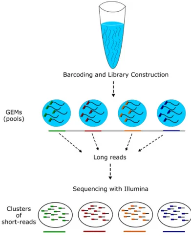
2.2 Details of 10x technology. Each step of 10x pipeline is briefly
de-picted. Firstly, 1 ng of high molecular weight DNA is extracted
from the sample and distributed to approximately 106 pools, where
they are barcoded and subjected to priming and polymerase am-plification. After the library preparation process, they undergo
Illumina sequencing process. . . 40
3.1 Figure shows the IGV [3, 4] visualization of a deletion event
predicted by TARDIS within 19:8,231,867-8,256,118 for CHM1 genome [5, 6]. Absence or decrease of read-depth within the
break-point is an indication of a deletion. . . 45
3.2 Read pairs mapped to the reference genome A) insertion signature,
B) deletion signature. . . 46
3.3 Figure shows the IGV output of an inversion event predicted by
LIST OF FIGURES xii
3.4 Inversion signature of the read pairs mapped to the reference genome. 49
3.5 An example of a false SV prediction is depicted in the figure. There
is a deletion event in the left mapping when the duplication in the genome is not considered. We need to check wheter any of the pairs hit the annotated transposon interval in order to make a correct
prediction since the MEI insertions can be underestimated. . . 50
3.6 The figure depicts the overview of MEI clustering approach we
uti-lize in TARDIS. (A) We first check the paired-end reads where one end maps to an annotated transposon and the other to elsewhere within the genome. (B) For such cases, we cluster the pairs that map to elsewhere in the the genome based on their orientations within an interval. Then we bring forward and reverse pairs to-gether inside the same cluster and treat them as paired-end reads
in order to detect the insertion breakpoints. . . 51
3.7 There are four different cases for mobile elements (copy events) in
direct orientation. The cases are based on the position of PBr, and
orientation of the mappings. . . 52
3.8 There are 4 different cases for mobile elements (copy events) in
inverted orientation. The cases are based on the position of PBr,
and orientation of the mappings. . . 53
3.9 For NUMT insertion, we check whether any of the pair maps to
mitochondria. Such cases is an indication of NUMT insertions
within the genome. . . 54
3.10 Relative abundance of complex SVs among the inversion calls re-ported in the 1000 Genomes Project [7]. 54% of predicted inver-sions are in fact inverted duplications and only 20% are correctly
predicted as simple inversions. . . 55
3.11 Figure shows the IGV output of a tandem duplication event
pre-dicted by TARDIS within 3:1,216,580-1,217,848 for CHM1 genome. 56
3.12 Tandem duplication signature of the read pairs mapped to the
reference genome. . . 57
LIST OF FIGURES xiii
3.13 IGV visualization of interspersed SD in A) direct orientation and B) inverted orientation. It should be clear that the signature in (A) is +/− and −/+, in (B) −/− and +/+. The first one is exactly the same as the signature of deletion and tandem duplication, the
second one as inversion. . . 63
3.14 The sequence signatures for interspersed SDs in (A) inverted (B)
direct orientations. . . 64
3.15 Figure shows some reads mapped to the reference genome with multiple mappings allowed. We also show how the reads align with some mismatches allowed. The nucleotides in red color are
the mismatches. . . 65
3.16 When aligning a read to a reference genome, some bases match, some don’t. SAM/BAM specification outputs this information in a CIGAR string. The position of the read aligned to the reference
is 0-based starting position of the alignment. . . 65
3.18 Split read signatures used by TARDIS to characterize SV types of deletion, novel sequence insertion, transposon insertion, inversion, tandem duplication and interspersed segmental duplication in di-rect and inverted orientations. Briefly, when a read is mapped to the reference genome, the SV is hidden inside the read and this is
resolved by splitting the read into two segments. . . 66
4.1 Comparison of deletion accuracy (>100 bp) between TARDIS and
LUMPY using NA12878 genome (a). We also provide a deletion length histogram (b) exhibiting the expected peaks at 300 bp and
5,900 bp for ALU and L1 deletions . . . 72
4.2 Receiver operator characteristic (ROC) curve for the comparison
of inversion predictions on CHM1 and CHM13 datasets. Overall, TARDIS achieves better area under the curve (AUC) statistics compared to the other tools. (a), (b) comparison of CHM1 and CHM13 predicted inversions using PacBio reads based on BLASR mappings. (c) validation of top predicted inversion of different
LIST OF FIGURES xiv
4.3 Comparison of top inversion prediction on NA12878 sample against
predicted and validated set of inversion of the same samples using
PacBio data from [8] . . . 74
4.4 a) Illumina signature for an inverted duplication, b) PacBio
vali-dation. . . 76
4.5 Alu insertion predictions in CHM1 and CHM13 datasets, compared
List of Tables
1.1 SV discovery algorithms that use short reads. . . 18
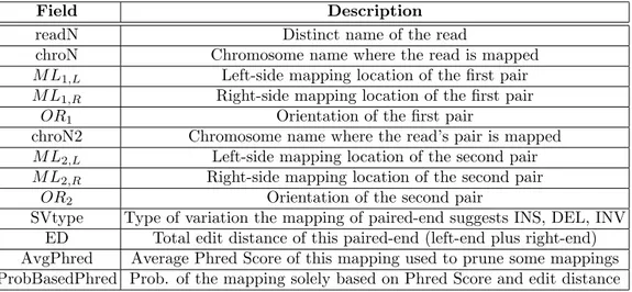
2.1 Mandatory fields of mrFAST output and how TARDIS handles
them. . . 31
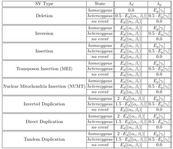
2.2 Formulation for λd and λp for maximum valid cluster Si . . . 38
4.1 Summary of simulation predictions by TARDIS, LUMPY and
DELLY. . . 69
4.2 Characterization of different types of segmental duplications using
TARDIS on simulated data. . . 70
4.3 Properties of the datasets we utilized in our eperiments. . . 71
4.4 Comparison of deletion accuracy between TARDIS, LUMPY and
DELLY using CHM1, CHM13 and NA12878 data sets . . . 71
4.5 50 highest scoring segmental duplications predicted by TARDIS in
the CHM1 genome. . . 75
4.6 Comparison of simulation predictions for Sensitive and Quick
Mode of TARDIS. . . 77
4.7 Comparison of real data (CHM1 genome) predictions for Sensitive
and Quick Modes of TARDIS. . . 78
4.8 Evaluation of Linked-Read performance of TARDIS. . . 79
Chapter 1
Introduction
To expose the mysteries of genome, various biological studies had been conducted in the past by researchers. With computational approaches today, we are able to make progress much more rapidly than before. Human Genome Project and 1000 Genomes Project are two milestones in biological research executed in the last 20 years, although they are not the only ones. With the introduction of high-throughput sequencing, the results of genomics became more valuable as this platform opened tremendous research opportunities to researchers.
1.1
DNA and Computational Genomics
The first clues of heredity in living organisms became evident in 1865 when Gregor Mendel explained how traits passed down from parent to child. A few years later, Friedrich Miescher identified “nuclein” in white blood cells of human, which is what we know as deoxyribonucleic acid today. Although the importance of Miescher’s findings was not realized for many years, Franklin, Watson and Crick’s description of the double helix structure of DNA [10] opened a new era in the field of genetics.
cell of living organisms. It has two long sequences of nucleic acids made up of four bases; Adenine (A), Thymine (T), Guanine (G) and Cytosine (C). These sequences are attached together by chemical bonds and are called base pairs; A pairs with T and C pairs with G on complementary strands.
DNA of an organism is packaged into structures called chromosomes inside the nuclei of cells. Human genome includes 46 chromosomes; 22 autosome pairs and two sex chromosomes that can be either XX or XY, for females and males respectively. The total length of these chromosomes is around 3 km in length and contains nearly 3.2 billion base-pairs (bp) with the addition of mitochondrial DNA (mtDNA) present inside the mitochondria that represents only a small fraction of the total DNA. These chromosomes and mtDNA contain the genes that code for proteins and human genome contains 20,000 to 25,000 of them. The combination of all the genes or the genetic makeup of an organism is what we call genome.
Human Genome Project (HGP) was launched in 1990 with the aim to sequence whole human genome and released the first results in 2001 [11]. This is a near complete human genome sequence created from the genomes of a few individuals and is called the “reference genome”. The project was completed in 2004 [12], but is still being updated. HGP attempt led to various new projects in the field of genomics [13, 14, 15, 16, 17, 18, 19, 20, 21], therefore the amount of data increased tremendously. With this increase, researchers were forced to rely on computational methods and subsequently new techniques and tools emerged. This can be regarded as the second birth of computational genomics area in the intersection of genomics and computer science.
1.2
Genomic Variation: Changes in DNA
Se-quence
Genomic variation is defined as the genomic differences between individuals. It has been shown that 99.9% of any two copies of human genomes are identical
(approximately 1 variant per 1,000 bases) [22, 23]. This minor variation causes biological differences between individuals and is what makes each unique. On the other hand, some of these variations are the causes of genetic diseases such as psoriasis [24], Crohn’s disease [25], renal disease [26], diabetes [26], AIDS sus-ceptibility [27], neurodevelopmental diseases (e.g., epilepsy, intellectual disability, autism, and schizophrenia) [28, 26, 29, 30] and many more. Thus, studying ge-nomic variations is crucial not only for most of the branches in molecular biology and genetics but also for medical sciences.
Genomic variations can be broadly classified into four groups based on their sizes; (1) Single Nucleotide Polymorphisms (SNPs) are the point mutations i.e., changes in one nucleotide of the genome; (2) INDELs are small insertions and deletions up to 50 bps and short tandem repeats (STR) are repeated small seg-ments up to approximately 171 bps; (3) Structural Variations are the genomic changes that affect more than 50 bps to several megabases; (4) Chromosomal changes that affect the whole chromosome i.e., trisomy or monosomy. The fre-quency of these variations are inversely proportional to their sizes.
In 2008, 1000 Genomes Project was launched to sequence the genomes of at least one thousand humans to create a catalog of human genetic variations using newer sequencing technologies. They launched the initial results in 2010 [14] and 2012 [18]. With the completion of the project in 2015 [20, 21], genomes of 2,504 individuals from 26 different populations were sequenced using predominantly Illumina technology, an integrated map of 84.7 million SNPs, 3.6 million INDELs, and > 65, 000 SVs were publicly reported. The project also revealed that a typical genome differs from the reference at around 4 million sites where more than 99.9% of these are SNPs or small INDELs and 2,100 to 2,500 of them are SVs.
There are also other genome sequencing projects [31, 32, 33, 34, 7] and among these Turkey has started a new project where the aim is to sequence and analyze 100,000 Turkish genomes in three years.
1.2.1
SNPs, INDELs and STRs
In 2001, The International SNP Map working group revealed 1.42 million SNPs in human genome [23] and in 2002, Intenational HapMap Project was initiated with the goal of determining the common patterns of DNA sequence variations in human genome by characterizing sequence variants, their frequencies and correla-tions among them [13]. In phase 1 of the project, 1.3 million SNPs and in phase 2, a further 2.1 million SNPs were genotyped and phased using 270 individuals from diverse populations [35, 36]. Thus, having these associations led to more accurate, faster and cheaper Genome Wide Association (GWAS) studies.
On the other hand, INDELs have not been studied as broadly as SNPs but they comprise 16% to 25% of all sequence polymorphisms in human genomes [37]. INDELs are known to cause phenotypic changes and diseases like cystic fibrosis [38] and fragile X syndrome [39]. There are some methods that dis-cover and genotype INDELs using high throughput sequencing datasets such as SPLITREAD [40] and Scalpel [41].
Finally, Short Tandem Repeats (STRs) are repetitive DNA motifs that consist of micro, mini, beta and alpha satellites that are utilized frequently in forensics, population genetics, and genetic genealogy [42]. They are also known to play an important role in genetic diseases such as various types of neurological disorders including Huntington’s disease [43]. Although detection of these events with computational approaches is very challenging, there are still some methods such as lobSTR [44] and hipSTR [45] that discover STRs.
1.2.2
Structural Variations
Structural Variations (SVs) are genomic rearrangements that affect >50 bps in the sequence of a genome including insertions, deletions, duplications, inversions,
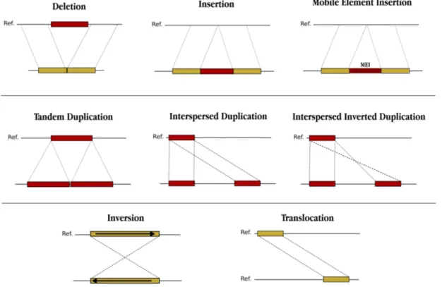
mobile element transpositions and translocations [46, 47, 48, 49, 2, 50] (Fig-ure 1.1). Among these, copy number variations (CNVs) are referred to as un-balanced structural variants that change the number of base pairs in the genome including insertions, deletions and duplications, whereas balanced rearrangements include inversions and translocations [51].
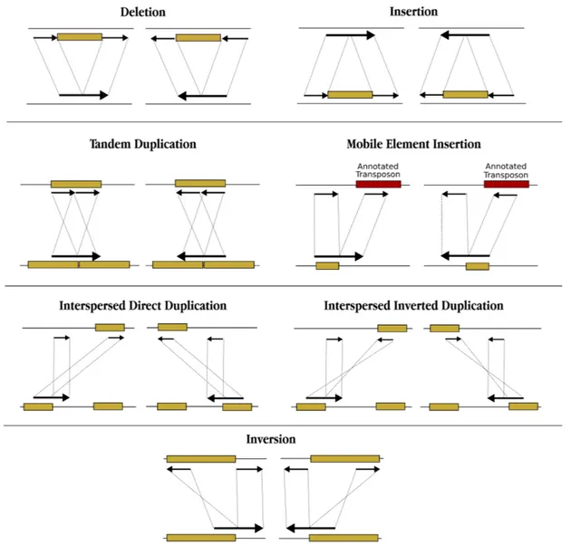
Figure 1.1: Structural Variations (SV) types of deletion, insertion, inversion, mobile element insertion (MEI), interspersed segmental duplication with direct and inverted orientations, tandem duplication and translocation are depicted.
There are various studies that associate SVs with genetic diseases ranging from neurological and neurocognitive disorders to autism, obesity, bipolar disorder, schizophrenia [52, 53, 54, 55, 56, 57] and cancer [58, 59]. Therefore the discovery and genotyping of SVs are of crucial importance in understanding their affects on human health.
The approaches to detect SVs can be broadly categorized into two groups; hybridization-based microarrays and sequencing-based computational ap-proaches.
1.2.2.1 Hybridization-based microarrays
Microarrays have traditionally been used for multiple purposes in molecular biol-ogy; gene expression, fusion gene profiling, alternative splicing, etc. Before high throughput sequencing, they were the main instruments for SNP, INDEL and CNV detection and genotyping [46, 47, 60, 61]. There are mainly two different methods; SNP microarrays and array comparative genomic hybridization arrays (arrayCGH) and they are both based on hybridization.
In arrayCGH, reference and test DNA samples are labeled with fluorescent tags and are hybridized to target genomic arrays (long oligonucleotides, bacterial artificial chromosome (BAC) clones are used for this purpose). After hybridiza-tion, the signal ratio reveals copy-number differences between the DNA samples. [62, 51].
On the other hand, SNP microarrays are used to find CNVs and single nu-cleotide polymorphisms in spite of the fact that their probe designs are specific to SNPs. They were mainly used in HapMap project to find millions of SNPs. Un-like arrayCGH, hybridization is performed on a single sample per microarray in SNP microarrays. Hybridization intensities and allele frequencies are compared with average values, which indicate a change in copy number.
In general, microarrays are cheap and fast, however, they have drawbacks; poor breakpoint resolution, always specific to a reference individual, not able to detect transposon insertions, novel sequence insertions and balanced rearrangements, i.e., inversions and translocations. They are also unreliable within segmental duplications.
There are additional approaches like polymerase chain reaction (PCR) used for SNPs, quantitative real-time PCR (qRT-PCR) for CNVs and fluorescent in situ hybridization (FISH) used for larger events [63, 64].
1.2.2.2 Sequencing-based computational approaches
DNA sequencing is the process of determining the order of nucleotides in a DNA molecule. This is a challenging task since there is currently no machine that takes a genome as input, reads it from start to end, and outputs the entire sequence.
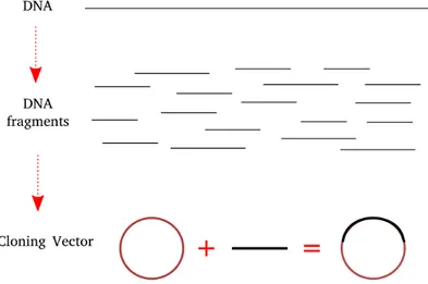
First attempts to sequence a genome involved breaking the DNA into many small pieces, sequencing them and assembling them again. As Figure 1.2 shows, DNA is cut into multiple fragments or inserts randomly where each fragment is sequenced using clones (Plasmids carry 3-7 Kbps, Fosmids carry ∼40 Kbps and BACs carry ∼150 - 200 Kbps). However, as entire clone cannot be sequenced, only some number of bases (∼1000) are sequenced and these are called “reads”. Sequencing can be done from rightmost, leftmost or both ends. Paired-end se-quencing is the process when the sequencer sequences from both left and right ends. It should be noted that the number of reads are redundant in order to reconstruct the original genome. As the redundancy increases, accuracy also in-creases and restoring the original genome becomes easier. This is called depth of coverage indicating the average number of reads that cover each base pair.
The history of DNA sequencing goes back to Gilbert [65] and Sanger [66] methods in 1977, where the first one is based on chemical sequencing and the latter on chain termination sequencing and both generate labeled fragments of varying lengths that are further electrophoresed. However, Sanger method gained more popularity and was used as the main sequencing tool in Human Genome Project.
Briefly, Sanger Sequencing relies on ddNTP, which is a modified nucleotide that can stop replication. As the DNA polymerase copies a DNA strand, when one of four dideoxy nucleotides (ddATP, ddGTP, ddCTP, or ddTTP), which lack a 3’ hydroxyl group, became incorporated instead of a dNTP, synthesis terminates. So four different test tubes containing a template DNA strand and a primer attached to it, a DNA polymerase, dNTPs and a few ddNTPs of the same type are used. Then, by using capillary gel electrophoresis, the molecules ending with ddNTPs with various different lengths are separated by size and then fluorescent tag on
each ddNTP are read in order to determine the nucleotides.
Figure 1.2: Sequencing approach employed by the first generation sequencers, i.e., Sanger Sequencing. Briefly, DNA is cut into multiple fragments randomly and each fragment is sequenced using clones.
Thus, Sanger sequencing allows long stretches of DNA fragments to be se-quenced (∼ 1000) with high accuracy using clone libraries, which can be used
in further processing. However, this technology is very expensive and slow.
Also, building and storing clone libraries is difficult and time consuming. With the introduction of next-generation sequencing (NGS), or currently called high-throughput sequencing (HTS), the field of genomics has been revolutionized. However, we should also note that the methods such as depth [67], read-pair [2] and split read [37] that we utilize with HTS technology today were first developed and used with Sanger sequencing technology.
1.3
High Throughput Sequencing
1.3.1
Short-read sequencing
Before 2005, Sanger sequencing, considered as the first generation sequencing platform, was the most feasible approach to sequence a genome harboring long
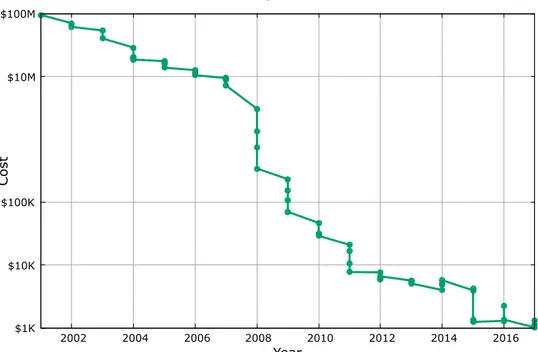
read length and high accuracy. However, newer sequencing platforms have emerged and changed genomics entirely as they are much faster and cheaper. Figure 1.3 shows the change of costs to sequence a genome between 2001 - 2017. The sudden decrease in 2008 displays the transition from Sanger sequencing to HTS [1]. It is noteworthy that sequencing a genome was around ∼ $100 million in 2001 and is only ∼ $1, 200 in 2017, a decrease of five orders of magnitude.
$1K $10K $100K $10M $100M 2002 2004 2006 2008 2010 2012 2014 2016 C os t Year Cost to Sequence a Genome
Figure 1.3: The change of cost to sequence a genome between years 2001 - 2017. Rapid decrease in 2007-2008 demonstrates the transition to HTS platforms. Data is retrieved from [1].
Main differences between the short-read sequencing and traditional Sanger se-quencing is that it produces up to billions of reads in parallel, which are much shorter (35 − 250 bps depending on the platform). Nevertheless, it has higher error rate and possesses bias against high and low GC contents. HTS platforms commonly utilize three main steps but differ in how they handle them; (1) tem-plate preparation; (2) sequencing and imaging; (3) data analysis [68]. Indeed, the fundamental difference between the commercial HTS sequencers is in terms of sequencing technology they utilize; 454 Life Sciences is based on pyrosequenc-ing, Illumina uses sequencing by synthesis and AB SOLiD employs sequencing by ligation.
There are two main approaches to analyze the reads of short-read sequencers: read mapping and de novo assembly. As both of these methods are highly complex and difficult to achieve, coupled with short nature of the reads, the problem gets even more difficult. Consequently, a combination of Sanger sequencing (longer read lengths) and HTS platform (faster and cheaper) was needed. 3rd generation sequencing (also known as long-read sequencing, single molecule sequencing or next-next generation sequencing) can be regarded as the result of this demand.
1.3.2
Long-read sequencing
Single molecule DNA sequencing was launched in 2008 with Helicos Biosciences [69], then Pacific Biosystems (PacBio) with Single Molecule Real-Time (SMRT) sequencing [70] and Oxford Nanopore Techniques (ONT) with nanopore sequenc-ing [71]. In contrast to 2nd generation sequencsequenc-ing, there is no clonal amplifica-tion step in library preparaamplifica-tion as they are able to detect single molecule in real time, i.e., the optics of these systems are very sensitive such that they can detect incorporation of one fluorescently labeled nucleotide [72].
Thus, 3rd generation sequencers have reduced PCR based errors, they have much longer read length (10-15 Kbps for PacBio and 6 Kbps for Oxford Nanopore) and they do not suffer from GC bias. Additionally, they are not slow either [73, 74, 75]. However, compared to short-read sequencers, their error rates are higher (0.1% for Illumina, 5−20% for Oxford Nanopore and 10−15% for PacBio) and they are much more expensive [76, 77, 78].
Currently, these sequencers are mostly utilized in de novo assembly algorithms such as FALCON [79], HGAP [80] and MHAP [81] and there are relatively few algorithms such as PBHoney [82], SMRT-SV [83], Sniffles [84] and HySA [85] for reference based SV detection.
1.3.3
Linked-Read sequencing
Recently, to overcome the limitations of short and long read sequencers, a new approach called Linked-Read sequencing developed by the 10x Genomics (10xG) company has been introduced. According to this approach, short reads are gen-erated with additional long range information producing Linked-Reads of tens of Kbs originating from the same haplotype [86, 87], obtaining high sequence coverages with the cost of generating moderate coverage data.
This new technology works by first partitioning large DNA molecules (typi-cally 10-100 Kbps) into partitions called GEMs or pools, that contain ≤ 0.3× copies of the genome (2-30 large molecules) with unique barcodes, which are then sequenced using Illumina sequencer. Looking at the barcode information of each read-pair, long range information can be deduced; sequences derived from the same molecule shares the same barcode, thus they are linked [88].
There are currently a few algorithms that use Linked-Reads to identify SVs. LongRanger [89] is one of the pioneering approaches developed by 10x Genomics, which is a comprehensive package capable of doing both sequence alignment and SV detection using barcoded reads. On the other hand GROC-SVs [90] focus on cancer genomes using Linked-Reads and is also able to detect complex SV events
employing local assembly. ZoomX [91], another algorithm that uses
Linked-Read sequencing, is able to identify complex genomic rearrangements (>200 Kbp) in somatic and germline cells. Finally VALOR [92] characterizes large (>500 Kbp) inversions using “split molecule” signature, which is a similar approach to traditional split reads, but having the additional advantage of spanning over repetitive regions.
1.4
Reference Based Analysis
1.4.1
Read mapping
Read mapping or read alignment is the process of aligning reads onto the ref-erence genome, only if available, in order to detect which part of the genome they likely originated from and expose genomic variations. However this problem is very challenging. First, ∼ 50% of the human genome is repetitive [93, 94] and it is impossible to know which copy of the repeat the read should belong to (ambiguity). Second, alignments may contain mismatches, which may be due to sequencing errors, genuine differences (SNPs, INDELs) between reference and query organisms, or both [95]. Indeed, in order to achieve higher accuracy, a confidence score (mapping quality) is needed for the alignments [96]. Finally, due to the huge number of reads, memory consumption will be very high and the speed of the algorithm will decrease. Therefore an optimal alignment (i.e., Smith-Waterman local alignment [97] algorithm) is not possible, so read map-ping algorithms apply heuristics. There are two main approaches; (1) hash based seed-and-extend aligners such as mrFAST [98], BFAST [99], mrsFAST [100], SHRIMP 2 [101], FASTHash [102], NovoAlign [103]; (2) Burrows-Wheeler Trans-form & Ferragina-Manzini Index based aligners PatternHunter 2 [104], Bowtie [95], BWA [105], Bowtie 2 [106].
Hash based aligners initially partition the reference genome into overlapping, equal sized k − mers and index them in a lookup table (i.e., hash table). When searching for the position of the reads, each read is also cut into k − mers sim-ilarly and these k-mers are used as keys to look up the matching positions in the reference. Once a match is found, it is extended to align the entire read. Although this approach is sensitive, it is very costly in terms of memory and it is computationally slow. Indeed, most of the time, more than 90% [107, 108], is spent in the verification step that is based on edit distance. Algorithms such as Levenshtein’s edit distance [109], Smith-Waterman [97] or Needleman-Wunsch [110] are used for this purpose [111].
On the other hand, Burrows-Wheeler Transformation (BWT) is a data com-pression method that is used to compress the genome, which can be used to reduce memory load. Utilizing this strategy, second type of aligners store a memory-efficient representation of the reference genome and use Ferragina-Manzini index data structure that retains the suffix array’s ability for rapid subsequence search [112]. Then, each read is aligned character by character against the transformed string [113]. By this way, hits can be found very quickly in a memory efficient manner with reduced sensitivity.
There are also other approaches that apply different strategies to map long reads such as LAST [114], BLASR [115], BWA-MEM [116], DALIGNER [117], GraphMap [118], MECAT [119], LAMSA [120], Minimap 2 [121] and NGMLR [84].
1.5
De novo Assembly
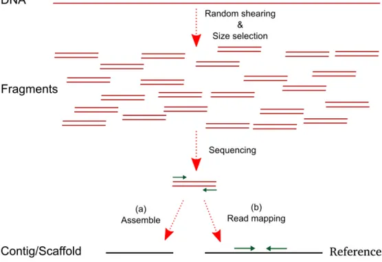
De novo assembly involves assembling the reads to reconstruct the original genome. However, this is currently an expensive task, comprising many chal-lenges. Shown in Figure 1.4, fragments are randomly sheared and expected to be overlapping with each other. Theoretically, entire genome can be assembled using the similarities of the overlapping parts inside the fragments and larger contiguous sequences called contigs, can be obtained [122]. The first challenge is the repetitive nature of the genome (∼ 50% of the human genome is repetitive). This becomes even more difficult with shorter read sizes; when the repeat element is larger than the read length, the algorithm cannot distinguish between the two copies. This results in gaps or missing sequence information.
Second, due to the heterozygosity of the genomes (human genome is diploid; 2 alternates of each locus), two inherited copies will have differences and both copies should ideally be constructed by the assembler. Third, because of the double helix structure of the DNA, reverse and complemented forms of the strings should be considered and sequencing errors need to be handled properly. Finally, similar
Figure 1.4: Whole Genome Shotgun (WGS) sequencing. Firstly, DNA is frag-mented randomly and then each fragment is sequenced from both left and right ends using a sequencer. These are called paired-end reads. The number of base-pairs that the sequencer reads called read length depends on the sequencing ma-chine used. Finally, the reads; (a) can be assembled into contigs when a reference genome is not available or (2) can be mapped to a reference genome
to most of the bioinformatics problems, size of the data is huge and there are billions of reads, therefore proper memory management is crucial.
First attempts to solve de novo assembly problem were formulized as shortest common superstring problem (SCS), which is known to be NP-Complete [123]. Given a collection of strings S = {s1, s2, ..., sn}, SCS asks to find the shortest
string s that contains all the substrings in S. Various heuristics or approximation algorithms for either SCS or its reductions to other NP-Complete problems such as Traveling Salesman and Hamiltonian path have been devised. Today three main approaches are being used: (1) Construction of contigs greedily (TIGR [124], PHRAP [125]); (2) Overlap-Layout-Consensus (OLC) (ARACHNE [126],
Phusion [127], PCAP [128], BOA [129]); (3) De-Bruijn Graphs (DBG) (EULER-SR [130], Velvet [131], EULER-U(EULER-SR [132], ABySS [133], Ray [134], SOAP-denovo [135], ALLPATHS-LG [136], [137], Meraculous [138], Cortex [139], SPAdes [140], HipMer [141]).
In the greedy approach, best matching prefix-suffix pairs are merged into longer sequences iteratively in a greedy manner. Most algorithms use overlap graphs or lists to keep the overlaps but generally these algorithms does not scale well with repeats (not appropriate for eukaryotic genomes, can be used for some bacterial or viral genomes).
OLC is composed of three main steps; in the “overlap” step, an overlap graph with prefix-suffix matches of all pairs of reads is created. The second step, called “layout”, consists of building contigs by passing over each node exactly once using Hamiltonian path or Traveling Salesman Path, which is NP-Hard. Finally, in the “consensus” step, consensus sequence is determined using multiple sequence alignment of overlapping contigs created in the second step. The main drawback of OLC is the huge and slow-to-build overlap graphs, which is inappropriate for 2nd generation sequencers that have billions of reads. They were mostly used for Sanger sequencing and currently have applications to 3rd generation sequencers [142].
De Bruijn graph (DBG) assembly is considered as the most appropriate
approach for short-read sequencing. Formally, given a set of reads S =
{s1, s2, . . . , sn} and an integer k, we define De Bruijn graph as G(S, k), where
the verticies are substrings of length k. There exists a directed edge between any two vertices u and v if and only if the last k − 1 characters of u is equal to the first k − 1 characters of v. Thus, the paths in the graph are the reads and a solution to the assembly problem is an Eulerian path that includes all reads as subpaths [143]. The assembler constructs the contigs using Eulerian walks in O(|E|) time where E is the number of edges. However, DBG also has drawbacks; sequencing errors (gaps, etc) or uneven coverage can make the graph non-Eulerian. Even if not, genomic repeats produce many possible walks (i.e., fragmented assemblies) [144].
All these assemblers create thousands to millions of contigs depending on the data. To help improve assembly contiguity, scaffolding algorithms are used that is the process of ordering and orienting these contigs with respect to each other using various data such as paired-ends. Usually assembler have scaffolding feature but there are also standalone scaffolding algorithms such as SSPACE [145], Opera [146], SCARPA [147], BESST [148] and LINKS [149].
1.6
Structural Variation Discovery Signatures
To detect structural variations, ideally two assembled genomes are needed; a genome that we seek to detect SVs (donor) and a second genome with no vari-ation (the reference). This way, a direct comparison of these two genomes will reveal the genetic variations trivially. However, because of the limitations of the current technology, we only have the reference genome correctly assembled (not 100% though) and chunks of the donor genome aligned to it (billions of reads). Therefore, we need to rely on signatures to detect structural variations. As Fig-ure 1.4 shows, sequencing machines generate two reads from both ends (start and end) of a fragment and these reads are called mate-pairs or paired-end reads. The distance between these two mates, called “insert size”, is the major data we have in order to utilize the sequence signatures in general.
There are four main signatures used to find SVs; (1) read-pair, (2) read-depth, (3) split read, (4) assembly; and all of these methods are based on the principle of aligning billions of reads to a reference genome and identifying potential SV events [150, 151]. However, there are complications with respect to specificity and sensitivity. The main problem lies in the repeated nature of the human genome. It comprises long segmental duplications and repeats where most of the potential SVs intervene with them. When using unique mapping of the reads, sensitivity decreases, whereas ambiguous mappings increases the false positive count. Additionally, incompleteness of the reference genome causes more prob-lems in accurate detection since these missing portions are mostly duplications. Second, many SVs are complex with many rearrangements at the same site. In
addition, tight breakpoint resolution is often difficult to achieve with specific se-quence signatures, besides, most of the smaller SVs (50 bp to 1 Kbp in length) cannot be resolved with short read sequencing [9]. Finally, short read sequencing approaches suffer from the GC bias (regions with elevated G plus C bases have higher read depth [152]).
First attempts to detect structural variations relied on similar approaches used in capillary sequencing [2, 153] and were able to detect only some basic types of SVs such as insertions, deletions, inversions and tandem duplications by using one of the sequence signatures. The following algorithms are some of the earlier approaches; (1) Read-pair signature based; VariationHunter [154], PEMer [155], BreakDancer [156], MoDIL [157], SVDetect [158], GASV [159] (2) Read depth signature based; CNVnator [160], EWT [161], mrCaNaVaR [98] (3) Split read signature based; Pindel [162], AGE [163] (4) Assembly based; NovelSeq [164], Cortex [139], SOAPdenovo [135].
On the other hand, newer approaches mostly utilize more than one sequence signatures to detect SV events and some are also able to characterize more com-plex variations. Table 1.1 shows state-of-the-art short-read sequencing algorithms that use Illumina platform to detect SVs by tracking multiple SV discovery sig-natures.
1.6.1
Read-pair
Read-pair (RP) method is the most widely employed approach and was first intro-duced in [153] for bacterial artificial chromosome end sequences generated from the breast cancer cell line MCF-7. Later, it was applied to discover germline genetic variation using fosmid paired-end sequencing [2]. Then, with the intro-duction of NGS, it was applied to short-read sequencing with 454 FLX platform [176] and then to Illumina.
The general strategy is based on aligning the paired-end reads to the reference genome and observing the distance, called “insert size”, between the pairs as
Table 1.1: SV discovery algorithms that use short reads.
Signatures
SV Types
DEL INS INV MEI NUMT TRA Duplication
TDUP ISP ISP-INV
CNVer(2010) [165] RP, RD X X X X X X X X X inGAP-sv(2011) [166] RP, RD X X X X X X X X X DELLY(2012) [167] RP, SR X X X X X X X X X GASVPro(2012) [168] RP, RD X X X X X X X X X PeSV-Fisher(2013) [169] RP, RD X X X X X X X X X LUMPY(2014) [170] RP, RD, SR X X X X X X X X X
Manta(2015) [171] RP, SR X X X X X X Xcannot distinguish
SV-BAY(2016) [172] RP, RD X X X X X X X X X
Pamir(2017) [173] RP, SR, AS X X X X X X X X X
TARDIS(2017) [174] RP, RD, SR X X X X X X X X X
SvABA(2018) [175] RP, SR, AS X X X X X X Xcannot distinguish
State-of-the art short-read sequencing algorithms that use Illumina platform are summa-rized in the table. We limit the algorithms to the ones tracking more than one sequence signature as none of the algorithms that use a single signature is comprehensive and newer approaches employ multiple signatures to increase sensitivity and specificity. Thus, for each algorithm, we give the sequence signatures it utilizes (RP, RD, SP, AS denote read-pair, read-depth, split read and assembly, respectively) and whether it is able to discover SV types of deletion (DEL), insertion (INS), inversion (INV), mobile element insertion (MEI), nuclear mitochondria insertion (NUMT), translocation (TRA), tandem duplica-tion (TDUP), interspersed segmental duplicaduplica-tion in forward (ISP) and reverse (ISP-INV) directions.
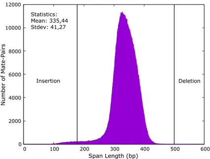
shown in Figure 1.5. Figure 1.6 shows the distribution of insert sizes (or span sizes) for NA11930 genome. If the insert size of a paired-end read is below the expected distance (∼ 170 bp in this example), there is a high possibility of an insertion event and larger insert size relative to the expected threshold (∼ 500 bp) is an indication of a deletion event relative to the reference genome.
In broad terms, algorithms that use read-pair sequencing use the term “discor-dant” for read-pairs whose insert size is smaller/larger than the expected interval when mapped to the reference genome. Also, “concordant” read-pairs are those having expected insert size, i.e., when the distance between the aligned reads is within the expected range. Therefore the algorithms that make use of read-pair method mostly deal with the discordant read-pairs as they indicate possible SV loci.
In addition to observing the insert size, if one of the pairs has an unexpected orientation, it’s likely the result of an inversion [2] and these read-pairs are also
Figure 1.5: Read-pair signatures of each SV event is shown. Reads are mapped to the reference genome and the distance between the mate-pairs or the orientation of the mapped reads determine whether a potential SV is implied or not.
classified as discordant. Note that reads should typically map in forward-reverse (+/−) orientation, which is considered correct mapping, i.e., the left mate is mapped to the “+” strand, and the right mate is mapped to the “−” strand. However, for inversions, one of the ends has flipped orientation, so +/+ or −/− mappings are tracked.
In case of tandem duplications, both ends map in everted (−/+) orientation. For mobile element insertions, the approach is different; if one of the mate pairs fall inside the annotated transposons, we see a potential mobile element insertion event. Finally, for interspersed segmental duplications, two types of mappings should be detected; +/− and −/+ for direct and +/+, −/− for inverted seg-mental duplications. However, these signals might not be enough for detecting interspersed segmental duplications as they are very similar to other types of SV events, so different types of signals or post-processing based on a likelihood model
0 2000 4000 6000 8000 10000 12000 0 100 200 300 400 500 600 Number of Mate-P airs Span Length (bp) Statistics: Mean: 335,44 Stdev: 41,27 Deletion Insertion
Figure 1.6: Span size distribution of read-pairs sampled from NA11930 genome. When the read-pairs are mapped to the reference genome, distance between them is a possible indication of a genomic variation. If the distance is below or above the expected cut-off values; min = mean − (4 × stdev) = 170, max = mean + (4 × stdev) = 500 in this case; then these read-pairs are called “discordant” and they are the ones considered as potential SVs [2].
might be needed.
1.6.2
Read-depth
Read-depth (RD) signature was first applied to old capillary sequencing data in order to identify duplications in human genome by [67]. It was later applied to HTS data to define rearrangements in cancer [177, 178] and then segmental duplication and absolute copy-number maps in human genomes [98, 179]. The general idea is simple and depends on the assumption that number of reads mapping to any region follows a Poisson distribution. Thus, by analyzing the divergence from this distribution reveals deletions or duplications in the sample. As displayed in Figure 1.7, deleted regions will have lower read-depth, whereas duplicated regions will have higher read-depth compared to regions of diploid nature.
Figure 1.7: Read-depth signatures of SV events are shown. When reads are mapped a region, divergence from the distribution implies a deletion (decrease in read-depth) or a duplication (increase in read-depth) event.
The accuracy of this method is highly correlated to the coverage of the dataset; with lower coverages, accurate SV detection will not be possible. Compared to read-pair approach, detection of larger SVs are possible with this approach, although smaller events that RP is able to detect with lower coverages might not be detected by RD signals [150]. As expected, breakpoint resolution of the method is poor. Finally, RD approach is highly affected by the sequencing bias of HTS technology, as some regions are over or under sampled mostly due to the GC bias.
1.6.3
Split read
The first application of split read (SR) signature was based on Sanger sequencing [37], and Pindel [162] was the first to apply it to HTS data. According to this method; when a read maps to a reference genome, there are some chunks of the read, mostly at the beginning or at the end, called soft clips, that cannot be mapped correctly. Split read approach involves remapping these chunks into the reference with gaps indicating a possible SV event (Figure 1.8).
This approach depends on read-length and is more successful when the reads are longer because they will be more likely to span SV breakpoints. Additionally, remapping of each split will be more accurate when read length increases as the difficulty of the alignment decreases.
1.6.4
Assembly
As described in Section 1.5, by assembling reads into DNA fragments (contigs), one can detect any type of genomic variations by comparing them directly to the reference genome. However, assembly (AS) is a hard problem such that the human genome is highly repetitive and consists of too many duplications [180, 181], which results in low-quality contigs. Thus, these drawbacks are prohibitive for using assembly to detect structural variations, although there are some assemblers that characterize SVs using de novo assembly, local or reference guided.
1.7
Contributions
In this dissertation, we present TARDIS (Toolkit for automated and rapid dis-covery of structural variants) that uses high-throughput sequencing technology to detect various types of genomic variations. TARDIS harbors novel algorithms to accurately characterize both simple and complex SV types including deletions, novel sequence insertions, inversions, transposon insertions, nuclear mitochondria insertions, tandem duplications and interspersed segmental duplications in direct or inverted orientations using short read whole genome sequencing datasets. Our algorithms make use of multiple sequence signatures including pair, read-depth and split read to find near-exact loci of each variation while resolving ambiguities among various putative SVs: 1) at the same locations signaled by different sequence signatures, and 2) in different locations signaled by the same mapping information. Additionally, TARDIS is able to analyze more than one possible mapping location of each read to overcome the problems associated with repeated nature of genomes. Finally, we extended TARDIS to be able to utilize Linked-Read information of 10x Genomics to overcome some of the constraints of short-read sequencing technology. TARDIS is the first method to predict insertion locations of complex SV events including tandem, direct and inverted interspersed segmental duplications. Using simulated and real data sets, we showed that it outperforms state-of-the-art methods in terms of specificity and demonstrates
comparable sensitivity for all types of SVs, and achieves considerably high true discovery rate for segmental duplications.
Before giving the details of our approach in the following chapters, we briefly describe two other state-of-the-art SV discovery tools, namely DELLY [167] and LUMPY [170] that we used to compare our results with. DELLY uses read-pair and split read signatures to characterize deletions, inversions, tandem du-plications and translocations. It utilizes an undirected graph based paired-end clustering, where each node in the graph denotes a paired-end read. The edges between the nodes indicate that both paired-end reads support the same SV and the edge weights denote the difference between the predicted SV sizes of the map-ping locations. It assumes that the graph contains one fully connected component for each SV and it could thus be identified by computing the connected compo-nents of the graph. However, this is an ideal condition, which is not possible in most cases, thus they identify maximum cliques heuristically in the components. In order to fine map the genomic rearrangements at single-nucleotide resolution, they utilize this information as input to their split read analysis.
LUMPY, on the other hand, has a module based probabilistic framework, which is able to discover deletions, inversion, tandem duplications and transloca-tions. It harbors read-pair, split read and a generic module to convert SV signals from each alignment to probability distributions assuming that they reflect the uncertainty in the reference genome that can be a potential end of a breakpoint, i.e., the split read module maps the output of a split read sequence alignment algorithm. The algorithm simply maps the evidences from the alignment signals to breakpoint intervals and the overlapping ones are put into the same cluster by integrating their probabilities. Finally, breakpoint regions with sufficient ev-idence is returned as SV predictions (If the alignments are not given as input, they utilize SAMBLASTER [182] to detect discordant reads and split reads using the input BAM file). Sites of known variants can also be provided to LUMPY as prior knowledge in order to improve sensitivity.
describing genomic variations, technologies of the past and the present, and ap-proaches used to detect genomic variations. Finally, we outlined our contributions shortly. In Chapter 2, we give an overview of our approach to the problem of structural variation discovery with TARDIS. In Chapter 3, details of structural variations and our approach to characterize them are given in detail. We present our results in Chapter 4 and finally conclude the dissertation by exploring poten-tial future research directions throughout Chapter 5.
Figure 1.8: Split read signatures of SV events are displayed. Here, unmapped reads are split and each fragment is remapped to the reference genome to observe potential SVs.
Chapter 2
Overview of TARDIS: Toolkit for
Automated and Rapid Discovery
of Structural Variants
2.1
Introduction
2.1.1
Motivation
Genomic variations are known to be the prominent source of genetic diseases. These variations range from single nucleotide polymorphisms (SNPs) that affect a single nucleotide as substitution, to small insertions/deletions (INDELs) up to 50 bp, structural variations that affect more than 50 bp and larger chromosomal alterations that alter the whole chromosome.
Beginning with the introduction of high throughput sequencing platforms, and later 1000 Human Genome Project (1000GP), several researchers focused on char-acterizing SVs in human genome. Thus a plenty of algorithms have been devel-oped. Compared to the previous approaches to detect SVs that involved using
BAC arrays, oligonucleotide array comparative genomic hybridization, SNP mi-croarrays and finally Sanger sequencing, speed and cost of HTS platforms are unimaginably low and they are able to detect plenty of SVs. As a matter of fact, with the completion of 1000GP, over 65, 000 SVs [20, 21] were reported, which was made possible with the algorithms that utilize HTS platforms.
However, these algorithms have considerable drawbacks as well; first, although they possess acceptable sensitivity, they have many false predictions. Second, they are able to discover only simple types of SVs such as insertions, deletions and short inversions as they cannot accurately characterize complex SV events. Indeed, this is one of the reasons for lower specificity they possess.
Earlier algorithms rely on using only one of the possible sequence signatures (read pair, read depth, split read or assembly). This results in fewer detectable SV types since each signature is capable of detecting only some specific SV classes. Additionally, using a single sequence signature reduces the precision of the al-gorithms as they have no way of verifying detected SVs by taking advantage of multiple evidence. On the other hand, newer approaches combine more than one sequence signature, however the second signature is mostly used as a post-processing approach for verification. Thus, since they aim to characterize only a few types of SVs, they do not try to resolve conflicting SVs within the same loci. Another weakness of these algorithms is that most of them consider only high confidence alignments and dismiss reads with lower quality alignments or reads with multiple possible mapping locations. Considering the repetitive nature of human genome, this naturally decreases the sensitivity of the algorithms within the repeated segments.
2.1.2
Our approach
Here we introduce TARDIS, a toolkit for automated and rapid discovery of SVs using both whole genome sequencing data (WGS) generated by Illumina platform and Linked-Read sequencing of 10x Genomics (10xG) [87]. However it can easily
be extended to support long read sequencing such as PacBio or Oxford Nanopore. The general framework to using paired-end reads to detect SVs between a reference and a donor genome was first formulated by [153] and [2]. It was based on a simple idea with two steps; (1) Mapping the paired-end reads to the reference genome; (2) Observing the orientations and distance of the discordant mappings.
When the read pairs are mapped to the reference genome, there are two signs that we track; span size and orientation of the pairs. First, the distance be-tween the pairs, called insert size or span size, is expected to be in some range
[δmin, δmax]. Read pairs within this range are categorized as concordant and the
ones that are below or above are called discordant. Indeed, discordant read-pairs suggest potential SV regions where larger or smaller insert sizes indicate deletions or insertions respectively. Second, orientation of the read-pairs are expected to be correct, i.e., +/− is the correct orientation for Illumina platform. Accordingly, the read-pairs with unexpected orientation are also designated as potential SVs such that −/− or +/+ are inversions and −/+ are tandem duplications.
Similar to most modern SV callers, TARDIS integrates multiple sequence sig-natures including read-pair, read-depth and split-read to accurately characterize both simple variants such as novel insertions, deletions, inversions, mobile element insertions, nuclear mitochondria insertions; and complex variants such as tandem duplications, direct and inverted interspersed segmental duplications (SDs) ac-curately. Besides, it resolves ambiguities such as; (1) Two or more SVs reported to be at the same location but signaled by different signatures; (2) Two or more SVs in different locations signaled by the same mapping information. However, current SV callers are incapable of characterizing several forms of complex SVs
such as tandem or interspersed segmental duplications (SDs) [183, 184] with
the exception of read-depth based methods that can only identify the existence of SDs [98, 179], but cannot detect breakpoints. TARDIS, on the other hand, is the first method to characterize insertion locations of segmental duplications using HTS data.
In this chapter we describe our approach to the problem of structural vari-ation discovery using HTS and leave the details of SV discovery to Chapter 4. The next section elucidates how we handle the mapping information (all possi-ble mappings of the reads to the reference vs. unique mappings) given as input to TARDIS. Then the details of the Maximum Parsimony Structural Variation approach (MPSV), adapted from [154, 185, 186] are given. Finally, we describe our approach using Linked-Read data.
Before proceeding, we give a brief description of the MPSV approach; It is a two-step process, where the first involves creating clusters with paired-end reads that suggest the same potential SV. Then in the second step, final alignments of each read-pair are determined by eliminating read-pairs from the clusters step-by-step. This is similar to the classical Set-Cover problem that is known to be NP-Complete, however [154] provides a greedy algorithm with an approximation factor of O(logn) using only the read-pair signature. TARDIS builds upon this approach, using the same objective function, but it also includes methodologi-cal and heuristic novelties; (1) incorporates split-read signature and adds novel paired-end reads to the clusters; (2) uses a probabilistic model that makes use of read-depth signature to assign a likelihood score to each potential SV.
We should also note that TARDIS is implemented in C using HTSlib and it is suitable for cloud use. Source code is also freely available at https://github. com/BilkentCompGen/tardis.
2.2
Read Mapping
In order to discover genomic alternations in a genome, the initial step constitutes mapping the reads belonging to a donor genome to the reference. Therefore, one can observe the variations from the reference genome. This preliminary step is achieved by using a read mapping algorithm. There are currently a vast amount of read mappers, which can be categorized based on various aspect such as the data structures they utilize, their output types, etc. Indeed, for SV discovery
algorithms, there is an important distinction between these read mappers. Some of them report only the best or an arbitrary mapping of the reads in case of a tied map locations such as MAQ [96], BWA [116], Bowtie [95] and some report all possible map locations such as mrFAST [98] and mrsFAST [100].
As we already know that most SVs lay within the repeated regions, consider-ing all possible mappconsider-ing locations of the reads is of crucial importance. There are currently some algorithms that utilize this information [187, 154, 188, 168]. Therefore the number of hits they have increase, although their specificity de-creases proportionally as some of these map locations might be incorrect. In addition to this, running time of these type of algorithms inherently increase, as searching for multiple map locations is a costly operation in terms of memory consumption.
In TARDIS, we possess two distinct modes of operation where the “Quick Mode” works only with the best mappings of each read-pair and “Sensitive Mode” deals with all the potential mappings.
2.2.1
Quick Mode
In order to interpret the mappings produced by a read mapper, TARDIS re-quires the mapper to utilize the well-known and most-widely used Sequence Align-ment/MAP (SAM) format and it needs the compressed and indexed BAM version [189] as input. The BAM file is composed of an optional header, that contains information about the reference that the individual has been mapped to, and an alignment section consisting of the actual alignments. Quick Mode of TARDIS utilizes the mapping information produced by BWA [116] or a similar aligner as input. It works by reading each mapping sequentially and deciding whether the mapping is a potential SV or not. Additionally read count and read-depth information is retained for read-depth analysis and yet, soft-clipped reads are manipulated for split reads.
![Figure 3.1: Figure shows the IGV [3, 4] visualization of a deletion event predicted by TARDIS within 19:8,231,867-8,256,118 for CHM1 genome [5, 6]](https://thumb-eu.123doks.com/thumbv2/9libnet/5555083.108305/60.918.173.791.169.470/figure-figure-shows-visualization-deletion-predicted-tardis-genome.webp)
