Coulomb effects in open quantum dots within the random-phase approximation
V. Moldoveanu1and B. Tanatar21National Institute of Materials Physics, P.O. Box MG-7, 077125 Bucharest-Magurele, Romania 2Department of Physics, Bilkent University, Bilkent, 06800 Ankara, Turkey
共Received 26 October 2007; revised manuscript received 7 April 2008; published 2 May 2008兲 The effect of electron-electron interactions on coherent transport in quantum dot systems is theoretically investigated by adapting the well-known random-phase approximation共RPA兲 to the nonequilibrium Green– Keldysh formalism for open mesoscopic systems. The contour-ordered polarization operator is computed in terms of the Green functions of the noninteracting system. We apply the proposed RPA-Keldysh scheme for studying Coulomb-modified Fano lines and dephasing effects in interferometers with side-coupled many-level dots. Our method allows us to treat on equal footing the decoherence induced by the intradot interaction and that by the Coulomb coupling to a nearby system. In the case of a single interferometer, we show that the intradot Coulomb interaction leads to a reduction of the Fano line amplitude. From the analysis of the inter-action self-energy, it follows that this effect originates in inelastic scattering processes in which electron-hole pairs are involved. The interplay between the interdot and the intradot interactions in decoherence is discussed for two nearby identical T-shaped interferometers. We also show that the intradot interaction does not prevent the observation of controlled dephasing due to a nearby charge detector, as long as the latter is subjected to a sufficiently large bias.
DOI:10.1103/PhysRevB.77.195302 PACS number共s兲: 73.23.Hk, 85.35.Ds, 85.35.Be, 73.21.La
I. INTRODUCTION
Understanding the role of Coulomb interactions in trans-port phenomena at nanoscale has become an imtrans-portant task for an accurate description of the underlying physics, espe-cially in the context of mesoscopic interferometry1and semi-conductor spintronics.2The reason is twofold. On one hand, the electron-electron interactions in highly confined systems such as quantum dot arrays are responsible for nontrivial effects that are appealing from the applications point of view 共Coulomb blockade,3–6 Kondo correlated transport,7 charge sensing,8,9 etc.兲 On the other hand, it was theoretically predicted10–12that the coherent features of transport are dam-aged by the inelastic processes due to the Coulomb interac-tion of the system with its environment. This statement was confirmed later on in the experiment of Buks et al.13 More precisely, it was reported that the Aharonov–Bohm oscilla-tions in a ring with an embedded quantum dot are partially reduced when a quantum point constriction subjected to a finite bias is placed near the quantum dot. Since the proper-ties of the constriction and of the dot are easily tunable, this decoherence process is also called controlled dephasing; it opened the way to indirect measurement techniques of quan-tum interference in mesoscopic systems. In contrast, the hy-perfine interaction between the electronic and nuclear spins sets undesired limits for solid-state implementation of quan-tum computation algorithms.14The problem of decoherence induced by intradot interactions was theoretically addressed by Sivan et al.15and by Altshuler et al.16
Since electron-electron interactions are a built-in feature of semiconductor nanostructures, considerable experimental efforts nowadays are focused on designing suitable quantum dot-based devices allowing the “reading” of interference ef-fects and the coherent manipulation of electrons while keep-ing the losses due to decoherence negligible. From the theo-retical point of view, the description of quantum transport in
interacting systems is not straightforward because one has to essentially deal with a many-body problem that leaves no room for an exact treatment except for very few simple mod-els. One crucial point then is to choose appropriate approxi-mation schemes for the Coulomb interaction in order to cap-ture subtle effects that play an important role in coherent or incoherent transport.
In this work, we propose a treatment of the Coulomb interaction based on the random-phase approximation共RPA兲 and on the Keldysh formalism, which we find useful in the study of dephasing in mesoscopic interferometers. Both the RPA and the Keldysh approaches are well established formal tools that lead to important progress in the description of two-dimensional electron gas properties and of the mesos-copic transport phenomena. In spite of this fact, the possibil-ity of combining them for studying open interacting systems driven by a finite bias has not been explored yet. In order to set the general context for our approach, we give in the fol-lowing a brief account of the Keldysh formalism and of its main applications. The main idea behind the nonequilibrium Green’s function formalism is to compute all relevant quan-tities of a system coupled to several biased leads by using the equilibrium state of the noninteracting disconnected system.17–19The coupling to the leads plays the role of the perturbation and is usually adiabatically switched. Then, a standard derivation leads to a closed formula for the current in terms of nonequilibrium Green functions. In the interact-ing case, the difficult and technical problem that remains to be solved is the calculation of these functions.
One approach is based on the equation-of-motion共EOM兲 method that was initiated by Zubarev20 and is extensively used by many authors in the study of Anderson and Kondo Hamiltonians 共see Refs. 21 and 22and references therein兲.
The usual strategy is to factorize the thermal averages of products of four creation共annihilation兲 operators in order to close the otherwise infinite chain of equations for higher-order Green functions 共see, for example, Refs. 23and 24兲.
One exactly solvable Fano–Kondo Hamiltonian within the EOM method is presented in a recent work.25
Another way to approximately compute interacting Green functions is to perform a perturbative expansion with respect to the interaction strength and to write down expressions for the first and second-order contributions to the interaction self-energy. This procedure successfully describes the con-trolled dephasing in mesoscopic interferometers Coulomb coupled to charge detectors.26,27This is because the second-order diagram for the interaction self-energy is the electron-hole bubble, which already takes into account inelastic pro-cesses that induce decoherence in the system. It should be mentioned that in this approach, a single-level quantum dot is considered and, therefore, the intradot interaction effect cannot be captured. König et al.28 argued that a single-particle approximation oversimplifies the role of the interac-tion and therefore cannot capture decoherence effects due to intradot Coulomb repulsion. Clarifying the role of interdot interactions in decoherence as well as the interplay between intradot and interdot interactions in controlled dephasing constitutes another motivation for considering the RPA-Keldysh approach to steady-state transport in interacting quantum dot systems.
We mention that Faleev et al.29 performed a self-consistent RPA calculation of the equilibrium Green func-tions and interaction self-energies for a homogeneous two-dimensional electron gas in the Kadanoff–Baym framework. Our approach is similar, the difference being that we con-sider open systems subjected to a finite bias and that the numerical simulations are done for lattice models. In a recent work, Wulf et al.30 calculated the admittance of one-dimensional open systems subjected to an additional ac bias superimposed to the source-drain bias. The steady-state re-gime of the system共that is, in the absence of the ac bias兲 is described within the Landauer formalism and the random-phase approximation is used to estimate the density change induced by the ac bias. Here, we study steady-state transport and focus on decoherence effects due to electron-electron interactions. We present two applications that are relevant to the dephasing problem in mesoscopic interferometers. The first model system we consider is a many-level one-dimensional quantum dot side-coupled to a single channel lead共the so-called T-shaped interferometer兲.
These systems attracted considerable attention since the observation of the Fano interference in the experiment of Kobayashi et al.31 Johnson et al.9 also reported different transport regimes of a quantum dot coupled to a single con-ducting channel: pure Coulomb peaks and charge sensing effect at very weak coupling to the channel or Coulomb-modified Fano lines at moderate coupling. The charge sens-ing effect allows measurements of Coulomb blockade with noninvasive voltage probes and requires a theoretical de-scription beyond the orthodox picture of the Coulomb blockade.32,33
The role of electron-electron interactions on the transport properties of side-coupled quantum dots has been theoreti-cally investigated especially in the context of the Fano– Kondo effect.34 Solving this problem requires nonperturba-tive techniques共such as the slave-boson mean-field theory or the renormalization group method兲 for dealing with the
on-site共Hubbard兲 interaction at the quantum dot, which leads to the strongly correlated Kondo state.35–37 Numerical or ana-lytical results have been obtained for single-level quantum dots only. On the other hand, Orellana et al.38 considered a one-dimensional side-coupled array of noninteracting quan-tum dots and found that the transport properties共resonances or antiresonances兲 depend on the number of sites in the array 共odd or even兲. The conductance is computed by using a re-cursive formula for the retarded Green function. Neverthe-less, to our best knowledge, no calculation of the Fano inter-ference for interacting many-level side-coupled dots has been done yet.
The paper is organized as follows: In Sec. II, we describe the method in a rather general form, in the sense that we do not specialize to the tight-binding Hamiltonian of a given structure. All we assume is that the electron-electron interac-tions are present only in some central region and not in the leads, as it is usually done in the Keldysh formulation of electronic transport. The spin degrees of freedom and the Kondo problem are not considered in this work. For the role of spin-flip effects in dephasing, we refer to the works of König and Gefen39 and of Silva and Levit.40In Sec. III, we show that the Fano interference is reduced when the Cou-lomb interactions inside the dot are taken into account. In the second half of Sec. III, we take two nearby T-shaped inter-ferometers and investigate in detail their coherence proper-ties in the presence of interdot and intradot interactions. The effect of a charge detector placed near the side-coupled quan-tum dot is also discussed. Finally, Sec. IV is devoted to con-clusions.
II. FORMALISM
In any theoretical approach to interacting quantum trans-port, one starts with a formal tool to write down a formula for the current through the considered system, in terms of the interacting quantities. The explicit results are then obtained by using approximation schemes for the interaction effects. Here, we use the nonequilibrium Keldysh formalism for electronic transport and the random-phase approximation for the Coulomb interaction. In view of the numerical imple-mentation, we shall work with tight-binding Hamiltonians. The system configuration is typical to the Keldysh approach: a central region共C兲 is coupled to noninteracting semi-infinite leads via a time-dependent switching共t兲. An adiabatic cou-pling is tacitly assumed in most of the theoretical calculations,17,41 which means that 共t兲 vanishes in the re-mote past, and the steady-state current is computed in the long-time limit. Actually, recent rigorous results show that the steady-state current does not depend on the way in which this coupling is achieved.42 Transient current calculations within the Keldysh formalism for noninteracting dots that are suddenly coupled to biased leads were also performed recently.43
We use the index␥ for the leads and di†共di兲 is the pair of
creation共annihilation兲 operators corresponding to the ith site of the lead. We also denote by al
†共a
l兲 the creation
共annihila-tion兲 operators on the lth site of the lattice describing the central region. Then, the system Hamiltonian quite generally reads
H共t兲 = Hcen+ Hleads+共t兲共Htun+ Hint兲, Hcen=
兺
l,m苸C 共l␦lm+ tlm兲al†am, Hleads= tL兺
␥ ⬍i,j⬎苸L兺
␥ di†dj, Htun=兺
i苸L␥l兺
苸C 共Vil␥di † al+ H.c.兲, Hint= U 2l兺
⫽m nˆlnˆm 兩rl− rm兩 . 共1兲In Eq. 共1兲, Vil␥ is the hopping coefficient between the
corre-sponding sites of the lead ␥ and of the central region. For simplicity, we take Vil␥to be real and nonvanishing only if i , l
are nearest neighbors. The last term in the Hamiltonian is written in terms of the on-site number operator nˆl= al†aland
describes the electron-electron interaction between charges localized in different sites of the central region. The interac-tion strength is characterized by the parameter U and rl
de-notes the position of the lth site. tLis the hopping energy on
leads, ⬍,⬎ denotes nearest neighbor summation and for simplicity the on-site energy of the leads is taken equal to zero.
Note that共t兲 switches both the coupling to the leads and the Coulomb interaction, which means that in our calcula-tion, the initial correlations are neglected.18,19 In the long-time limit when the system achieves a steady state, this ap-proximation is permitted. Finally, tlm are nearest neighbor
hopping parameters inside the central region and the on-site energieslmay include a constant gate potential Vg.
The standard application of the Keldysh machinery leads to the following preliminary formula for the current through the lead ␣in the steady state of the system:
J␣= e
បi苸L
兺
␣,m苸C冕
=⬁⬁
dE Re关Vmi␣Gim⬍共E兲兴, 共2兲
where Gmi⬍共E兲 is the Fourier transform of the lesser Green
function Gmi⬍共t,t
⬘
兲=i具ai†共t兲dm共t兲典. Note that the operators arewritten in the Heisenberg picture with respect to the total Hamiltonian and that we assumed the steady-state regime so that the Green function depends only on time differences. At this point, one has to express the mixed index Green function according to the Langreth rules,18
Gli⬍=
兺
␥ j兺
苸L␥m兺
苸C 共Glm R Vmj␥ g⬍ji+ Glm⬍Vmj␥gji A兲, 共3兲where gA,⬍ are the advanced and lesser Green functions of
the semi-infinite leads that are known共see, for example, Ref.
44兲.
Substituting their expressions into Eq. 共2兲, one ends up
with the following 共we omit the energy dependence for the simplicity of writing兲:
J␣=ie ប
冕
−2tL2tL
dE Tr关⌫␣共GR− GA兲f␣+ G⬍兴. 共4兲
In Eq. 共4兲, the Green functions are to be understood as
ma-trices and the trace means a sum over all sites of the central region. f␣ is the Fermi function of the lead␣ and ⌫␣ is a matrix linewidth, which is essentially given by the density of states in the lead,共E兲=共兩E兩−2tL兲
冑
4tL2− E2/2tL, and by thehopping constant between the lead ␣ and the central region 关共x兲 is the step function兴,
⌫lm␣共E兲 = 2Vil␣Vjm␣共E兲. 共5兲
Equation共4兲 was obtained for the first time by Jauho et al.41 and has been widely used in transport calculations for both interacting and noninteracting structures. In the noninteract-ing case, the perturbation comes only from the couplnoninteract-ing to the leads, whose self-energy is known,
⌺L,lm R 共E兲 = V li ␣V mj ␣ Im g ij R共E兲, 共6兲 ⌺L,lm⬍ 共E兲 = 2iVli␣Vmj␣ gij⬍共E兲. 共7兲
When the Coulomb interaction is taken into account, the main technical task is to compute, within appropriate ap-proximations, the interacting self-energy⌺I that should then
be plugged into the Dyson and Keldysh equations, GR= G0R+ G0R共⌺L R +⌺I R兲GR , 共8兲 G⬍= GR共⌺L⬍+⌺I⬍兲G A , 共9兲
where G0R,⬍are Green functions of the noninteracting discon-nected system. Using the known identity 共see Ref. 45兲 GR
− GA= 2iGRIm共⌺ L R
+⌺I
R兲GA and the Keldysh equation, one
obtains J␣=e h
冕
−2tL 2tL dE Tr关⌫␣GR⌫ GA共f␣− f兲 − ⌫␣GRIm共⌺I⬍ + 2f␣⌺I R兲GA兴. 共10兲This is an alternative form for the current that is particularly useful for emphasizing the limitations of the Landauer for-mula when applied to interacting systems.
One notices at once that the first term in the current has a Landauer form in spite of the fact that the Green functions appearing there are interacting quantities. The second term is given by the imaginary part of the interaction self-energy. In our previous work,27 we used the above formula to investi-gate the controlled dephasing in single-dot Aharonov–Bohm interferometers Coulomb coupled to a charge detector. The self-energy was computed by a perturbative approach up to the second order in the interaction strength.
Here, we propose an alternative method to compute the interaction self-energy based on the random-phase approxi-mation. The starting point of the RPA scheme is to construct the polarization operator ⌸. In the non-self-consistent ver-sion of the RPA that we implement here, the polarization operator is built from the noninteracting Green functions of
the coupled system. We denote these functions by Geffand
compute them by the Dyson equation共in the Keldysh space兲 with respect to the self-energy of the leads,
Geff= G0+ G0⌺LGeff. 共11兲
Since the Green functions we deal with are contour or-dered, the polarization operator⌸ has also lesser and greater components, besides retarded and advanced ones 共k,l are sites from the central region兲,
⌸kl共t1,t2兲 = − Geff,kl共t1,t2兲Geff,lk共t2,t1兲. 共12兲
Using the rules for diagrammatic expansion of the Keldysh– Green function, one is led to direct and exchange terms de-fined by the following RPA self-energies 共the corresponding diagrams are given in Fig.1兲:
⌺˜kl共t1,t2兲 = iVkl共t1,t2兲Geff,kl共t1,t2兲, 共13兲 ⌺˜ ˜ kk共t1,t2兲 = − i
兺
l Vkl共t1,t2兲Geff,ll共t2,t2兲, 共14兲where k , l denote sites from the central region and time ar-guments run along the two-branch Keldysh contour. V is the screened potential that obeys the Dyson equation with re-spect to the polarization operator⌸,
V共t1,t2兲 = V0共t1,t2兲 +
冕
dt冕
dt⬘
V0共t1,t兲⌸共t,t⬘
兲V共t⬘
,t2兲.The above integrals are along the Keldysh contour and we introduced the instantaneous bare Coulomb potential,
V0,kl共t,t2兲 = U 兩rk− rl兩
␦K共t1− t2兲, 共15兲
where the delta function is defined on the Keldysh contour 共see, for example, Ref.19兲,
␦K共t1− t2兲 =␦共t1− t2兲3, 3=
冉
1 0
0 − 1
冊
. 共16兲 Note that on each branch of the Keldysh contour K, the Cou-lomb interaction is instantaneous and also that it does not couple different branches on the contour. Using again the Langreth rules, one obtains explicit expressions for lesser and retarded quantities while the integrals are to be per-formed on individual pieces of the Keldysh contour. The retarded polarization is computed via the Kramers–Königre-lation and then the two basic equations for the polarization operator become ⌸kl⬍,⬎共E兲 = − 1 2i
冕
dE⬘
Geff,kl ⬍,⬎共E⬘
兲G eff,lk ⬎,⬍共E⬘
− E兲, 共17兲 ⌸R共E兲 = i 2冕
dE⬘
⌸⬎共E⬘
兲 − ⌸⬍共E⬘
兲 E − E⬘
+ i0 . 共18兲 Noticing that the integration range in Eq.共17兲 is restricted to关−2tL, 2tL兴 and that Green function is nonvanishing only if
兩E
⬘
− E兩⬍2tL, it follows that E苸关−4tL, 4tL兴. At the next step,one has to compute the RPA interaction according to the Dyson and Keldysh equations,
VR共E兲 = V
0+ V0⌸R共E兲VR共E兲, 共19兲
V⬍,⬎共E兲 = VR共E兲⌸⬍,⬎共E兲VA共E兲, 共20兲 where in Eq. 共20兲 we have used the property V0⬍= 0. The self-energies are then given by the following set of equations 共the argument E covers the interval 关−2tL, 2tL兴, as required
by the integral in the current formula兲:
⌺⬍,⬎共E兲 = ⌺˜⬍,⬎共E兲 + ⌺˜˜⬍,⬎共E兲, 共21兲
⌺˜kl⬍,⬎共E兲 = i 2
冕
dE⬘
Vkl ⬎,⬍共E⬘
兲G eff,kl ⬍,⬎共E − E⬘
兲, 共22兲 ⌺˜ ˜ kk ⬍,⬎共E兲 = − i 2冕
dE⬘
兺
lGeff,ll⬍,⬎共E
⬘
兲Vkl⬎,⬍共E兲, 共23兲⌺R共E兲 = i
2
冕
dE⬘
⌺⬎共E
⬘
兲 − ⌺⬍共E⬘
兲E − E
⬘
+ i0 . 共24兲 A particular feature of the RPA-Keldysh scheme is that the usual first order, direct, and exchange diagrams are not recovered when the RPA potential is introduced in the ex-pressions for ⌺˜ and ⌺˜˜. The reason for this is the following: the self-energies contain the lesser and greater components V⬍,⬎, which are given by the Keldysh equation whose first term is of order 2 in the bare Coulomb potential. This is different from the equilibrium version of RPA, wherein the self-energy contains the retarded component of the screened potential whose Dyson expansion starts with the first-order term. Therefore, we have to add by hand the first-order dia-grams in the final result for the retarded self-energy,⌺˜kl R共E兲 = i 2
冕
dE⬘
Geff,kl ⬍ 共E − E⬘
兲V 0,kl共E⬘
兲, 共25兲 ⌺˜˜kk R共E兲 = − i 2冕
dE⬘
兺
l⫽k Geff,ll⬍ 共E⬘
兲V0,kl. 共26兲 Equations 共25兲 and 共26兲 were obtained by again using thediagrammatic expansion and the Langreth rules. Note that in Eq. 共26兲, the integrals are actually decoupled and that
Im⌺˜˜kk R
= 0. Also,⌺˜R is off-diagonal because Vkk= 0 by
defi-k l k
FIG. 1. The two types of diagrams contributing to the interac-tion self-energy. The solid lines represent noninteracting Green functions Geffcalculated in the presence of the leads and the wiggly line is the RPA potential.
nition. Another useful quantity is the occupation number of the system, which is computed as usual from the lesser Green function 共i runs over all sites of the quantum dot兲,
N = − i 2
兺
i冕
−2tL 2tL dEGii⬍共E兲 =冕
−2tL 2tL dEN共E兲, 共27兲 where N共E兲 is the density of states.We end this section with some comments about the ex-pected range of validity for the RPA approach presented here. As pointed out by Henrickson et al.,44 first-order self-consistent calculations break down when the interaction strength exceeds the hopping constant on leads. This is be-cause in this range, elementary excitations are not captured by the perturbative approach. In a very recent work,46 the density of states for interacting electrons in graphene was calculated within the RPA and no plasmonic excitations were reported. In the numerical simulations presented in Sec. III, the interaction strength is always much smaller than the hop-ping constant of the leads.
III. APPLICATION TO DEPHASING IN T-SHAPED INTERFEROMETERS
In this section, we use the above RPA-Keldysh scheme to study the transport properties of a quantum wire with a side-coupled quantum dot. The specific system we shall study is a one-dimensional quantum dot having two sites, one of which is coupled to a single channel lead. In order to compare the effects of interdot and intradot interactions, we consider also two such interferometers that are Coulomb coupled when placed close to one another 共see the sketch in Fig.2兲. The
on-site energies of the dots are denoted by m共upper
inter-ferometer兲 and m 共lower interferometer兲, m=1,2, and the
hopping constant between the dots and the leads is denoted by . The sites of the leads where the dots are coupled are characterized by the on-site energy 0 and 0. The Hamil-tonian of the system then reads as
Hcen=
兺
m=1,2 关共m+ Vg兲am†am+共m+ Vg⬘
兲bm†bm兴 + tD共a1†a2 + b1†b2+ H.c.兲 +共a0 † a1+ b0 † b1+ H.c.兲 Hint=U 2l,m,l兺
⫽m nˆlnˆm rl− rm , 共28兲 Htun= tLa0 †共d 0␣+ d0兲 + tLb0 †共d 0␦+ d0␥兲 + H.c. 共29兲The annihilation and creation operators for the upper and lower interferometer are denoted by am, am
† and b
m, bm
†. Also,
we use the notations a0, a0 †
and b0, b0 †
for the operators asso-ciated with the two sites on the leads where the dots are attached. The hopping constant between the sites of the dots is tD, while tLis the hopping energy between the leads and
the central region. 0,=␣, ..,␥is the first site of the lead nu that is attached to the central region. We take m=mto be
the energy reference. Vg and Vg
⬘
simulate gate potentialsap-plied on the dots. The last term in the Hamiltonian contains both the interdot and the intradot interactions between the two dots. Htunis the tunneling term between the leads and the
system. We can also include the interaction between the dot and the neighboring site of the lead but this is not essential for our discussion. The bias, the energy, the hopping con-stants on the leads, the coupling and interaction strengths, and the gate potential will be expressed in terms of the hop-ping energy tD of the dots, which is chosen as the energy
unit. The hopping energy on leads is tL= 2tD, leading to a
bandwidth of the leads W = 8tD 共recall that the spectrum of
the semi-infinite one-dimensional lead is 关−2tL, 2tL兴兲. The
numerical simulations were performed in the very low-temperature regime kT = 10−4.
A finite bias is applied on the leads, i.e., V =␣− and V
⬘
=␥−␦, where ␣, . . . ,␦ are the chemical potential of the semi-infinite leads. We apply the bias in a symmetric way with respect to zero, that is,␣,=⫾V/2 and␥,␦=⫾V⬘
/2. All the curves we present below were obtained by using a suitable grid for the energy range in the integrals in order to obtain stable results. Typically, one needs 1500 points in the range关−4tL: 4tL兴. The main care here is to take properly intoaccount the very sharp peaks of the Green functions of the noninteracting system.
We first look at the role of the intradot interaction and consider only one interferometer. In Figs.3共a兲and3共b兲, one finds the first and the second Fano line shapes of the current as a function of the gate potential Vg. The bias is fixed 共V
= 0.2兲 and for the interaction strength we choose U = 0.1, 0.2, 0.3. We present the two peaks in separate plots in order to better discern the dephasing effect. The Fano pattern of the current as a function of the gate potential applied on the lateral dot originates in the interference between elec-tronic waves freely passing through the wire 共forming the so-called background signal兲 and waves that are scattered at least once at the side-coupled dot共the resonant contribution兲. It is clear that in the interacting case, both the amplitude and the shape of the asymmetric Fano line change. A small re-duction of the peak is seen but the main differences appear in the region of the Fano dip. At U = 0.1, the dip is pushed above the noninteracting one, but it almost disappears at U = 0.2. When further increasing the interaction to U = 0.3, the first Fano dip is recovered and a local maximum develops on its left side. In contrast, the second dip is even more dam-aged. Below, we shall discuss these features in more detail. Figure 3共c兲shows the density of states in the dot as a func-tion of energy and gate potential in the case U = 0.2. It is clear that at resonances共i.e., at Vg⬃−1 and Vg⬃1兲, the dot
G G G G G G α β γ δ ε ε ε 0 1 2 0 1 2 λ λ λ
FIG. 2. Schematic of two T-shaped interferometers. The nota-tions are explained in the text.
loses one electron as the localized states enter the bias win-dow关−0.1:0.1兴. This is why the two traces in Fig.3共c兲 dis-appear at energies E⬎0.1. We have also performed numeri-cal simulations for three- and four-site quantum dots and qualitatively obtained the same results.
We emphasize that a similar dephasing effect was ob-tained in our previous work,27 but there the effect was en-tirely due to the Coulomb interaction between a single-site dot embedded in an Aharonov–Bohm ring and a nearby de-tector. Here, it is the intradot interaction that leads to deco-herence.
We extend our analysis by showing in Figs.4共a兲and4共b兲 the current through the interferometer for fixed bias V = 0.1 and different signs of the Fano parameter. More precisely, the Fano parameter q is positive共i.e., the dip is located to the left side of the peak兲 if the on-site energy of the contact site 0= −0.75 and negative if0= 0.75. We plot also the separate
contributions of each term in the current formula关Eq. 共10兲兴.
The second term gives just a “bump” around the Fano reso-nance and we shall denote this contribution by Ji as it is
entirely due to the electron-electron interaction. The asym-metric shape of the resonance is given by the first term, which is proportional to the difference of the Fermi func-tions. Since in the noninteracting case this term is related to the Landauer formula for the conductance, we use the nota-tion Jc.
In both Figs. 4共a兲and4共b兲, a reduction of the Fano line amplitude is noticed in the presence of electron-electron in-teraction. The line shapes move to the right, which is essen-tially due to a Hartree-type shift from the interaction self-energy. Another observation is that the second Fano resonance is less affected by the Coulomb interaction, its shift being also smaller than in the case of the first Fano line. This happens because there is more charge in the side-coupled quantum dot before the first resonant tunneling. It is well known that at resonance the occupation number N of the
0 0.05 0.1 0.15 0.2 -1.4 -1.2 -1 -0.8 -0.6 -0.4 -0.2 0 Current Gate potential 0 0.05 0.1 0.15 0.2 0 0.2 0.4 0.6 0.8 1 1.2 1.4 Current Gate potential 0 10 20 30 40 50 60 Energy G ate potential -1.5 -1 -0.5 0 0.5 1 1.5 -2 -1.5 -1 -0.5 0 0.5 1 1.5 2 (b) (a) (c)
FIG. 3. 共Color online兲 共a兲 The first and 共b兲 the second Fano line shapes of the current through the interferometer as a function of the gate potential for different values of the interaction strength: full line, U = 0.3; dashed line, U = 0.2; dotted line, U = 0.1; long-dashed line, U = 0.0.共c兲 The density of states in the dot as a function of energy and gate potential 共see the comments in the text兲. Other parameters: V = 0.2,=0.35, =−0.75, and tL= 1. 0 0.05 0.1 0.15 0.2 -2 -1.5 -1 -0.5 0 0.5 1 1.5 2 C urrent Gate potential 0 0.05 0.1 0.15 0.2 -2 -1.5 -1 -0.5 0 0.5 1 1.5 2 C urrent Gate potential (b) (a)
FIG. 4. 共Color online兲 共a兲 The contribution of the two terms in the current formula for different signs of the Fano parameter共a兲 q ⬍0 and 共b兲 q⬎0. Full line, the total current; dashed line, the Lan-dauer current Jc; long-dashed line, the correction Ji; dotted line, the noninteracting Fano line. Other parameters: U = 0.2 V = 0.2, = 0.35, and tL= 1.
dot decreases by 1 over a range that roughly equals the reso-nance linewidth. Now, clearly, the first Fano line corresponds to the transition 2→1 and the second one develops as the quantum dot is emptied i.e., 1→0 关see also the density of states given in Fig.3共c兲兴. It is therefore understandable that the Coulomb effects are weaker on the second resonance.
The above comments apply to both Figs. 4共a兲and 4共b兲. Now we discuss the details of dephasing. When q⬍0 关Fig.
4共a兲兴, the suppression of the Fano line is mainly due to the enhanced value of the dip at U = 0.2. The reason is evident when we look at the two contributions to the current. On one hand, Jcalready displays a dip that is higher than the
nonin-teracting one, and on the other hand, the correction Jiadds to
the final value of the dip. Note that the Fano peaks are not drastically affected and that contribution of Ji decreases on
the second resonance.
Turning to Fig. 4共b兲 in which q⬎0, we observe that the suppression of the first Fano interference is symmetric, in the sense that the dip is enhanced and the peak diminishes. It is also interesting to mention that the contribution due to Ji
differently affects the two types of interference共constructive or destructive兲. In contrast to Fig.4共a兲where the maximum of Jiis located below the Fano dip, in Fig.4共b兲 this point is
rather below the Fano peak. As a consequence, the total peak is higher than Jcand the Fano dip is lower than the one in Fig.4共a兲. Nevertheless, when comparing to the noninteract-ing Fano line, we see that a dephasnoninteract-ing still exists. For the second line shape, the constructive interference 共i.e., the Fano peak兲 is reduced and the destructive one is not changed. The correction is again present but it does not change either the peak or the dip and affects rather the middle of the Fano line.
The above discussion suggests that in the presence of an intradot interaction, both constructive and destructive Fano interference are affected and that their sensitivity depends on the sign of the Fano parameter, that is, on the order in which the two types of interference are experienced by the system. If q⬍0, the destructive interference appears first and the interaction effects are predominant. If q⬎0, the Fano peak amplitude reduces and the Fano dip is less affected.
Now, we discuss the behavior of the interaction self-energy, which will shed some light on the main processes that induce decoherence in the system. For this, we have to consider the various matrix elements of⌺I.
In Fig. 5共a兲, we give the imaginary part of the retarded self-energy at the first site as a function of energy and gate potential关for a better visibility of Fig.5共a兲, we actually plot −Im⌺I,11兴. It is evident that at a very small temperature, it
suffices to restrict the energy range to 关−0.1:0.1兴, which equals the bias window共we take␣= 0.1 and= −0.1兲. One observes that the main contribution to the imaginary part corresponds to gate potentials that are located around the two resonances. We remark that the maxima of the self-energy have rather equal heights but they are not aligned in energy. Actually, the maximum around the second resonance is not centered in the bias window. A similar behavior is obtained for −Im⌺I,22. The imaginary part of the off-diagonal element
⌺I,12plotted in Fig. 5共b兲 is much smaller than the diagonal
counterpart. This is expected because for long-range poten-tials, as it is the case here, the exchange diagrams can be
neglected with respect to the direct contribution.47Note that Im⌺I,12is both positive and negative.
The imaginary part of the retarded self-energy is related to the inverse of the quasiparticle lifetime. In our case, there are two contributions to the resonance width: one comes from the leads’ self-energy ⌺L
R
and is roughly on the order of O共兲2 and the other one is entirely due to the Coulomb
re-pulsion. From the diagrams that correspond to Im⌺I,11, it
follows then that the dephasing in the upper interferometer, say, is mainly due to the interaction with at least one electron-hole pair that is excited in either one of the two subsystems. We recall that the creation and destruction of the electron-hole pairs are inelastic scattering processes.
In what concerns the real part of the interaction self-energy, it is responsible for the shift of the resonance and the main contribution is given by the Hartree diagram 关see Eq. 共26兲兴. This diagram contains the on-site occupation number
that is constant except at resonance when electrons escape from the dot to the side-coupled leads. This behavior is eas-ily checked in Fig. 6共a兲. Note that this term is energy inde-pendent since the involved scattering process is elastic. For completeness, we show in Fig. 6共b兲 the real part of the ex-change self-energy ⌺I,12. Again, it is smaller than Re⌺I,22.
In the following, we investigate the transport properties of two identical T-shaped interferometers that are mutually coupled via the Coulomb interaction between the side-coupled dots. If not otherwise stated, all interactions 共inter-dot and intra共inter-dot兲 are taken into account. We take the same lead-dot coupling strength on both systems. When the inter-ferometers have the same set of parameters, their Fano line shapes coincide. In Figs.7共a兲and7共b兲, we compare the
sec-0.05 0.04 0.03 0.02 0.010 -0.4 -0.2 0 0.2 0.4 -1.5 -1 -0.5 0 0.5 1 1.5 0.05 0.04 0.03 0.02 0.01 0 Self-energy Energy Gate potential Self-energy -5 -2 x 10 -5 -1.5 x 10 -5 -1 x 10 -6 -5 x 100 -6 5 x 10 -5 1 x 10 -0.4 -0.2 0 0.2 0.4 -1.5 -1 -0.5 0 0.5 1 1.5 -5 -1.5 x 10 -5 -1 x 10 -6 -5 x 10 0 -6 5 x 10 Self-energy Energy Gate potential Self-energy (b) (a)
FIG. 5. 共Color online兲 共a兲 −Im ⌺I,11R as a function of energy and gate potential. The important contribution comes from energies in-side the bias window关−0.1:0,1兴 and for gate potentials at which the Fano resonances appear.共b兲 Im ⌺I,12R as a function of energy and gate potential. Other parameters: U = 0.2, Vsd= 0.2,=0.35, and tL
ond Fano resonance in this case to the similar curve from Figs. 4共a兲 and 4共b兲. The dephasing is now given by both intradot and interdot Coulomb interactions. Overall, the Fano lines are similar to the ones obtained for the single interfer-ometer but several differences appear: 共i兲 The Fano lines of the Coulomb-coupled interferometers are shifted even fur-ther to the right when compared to the single interferometer case. 共ii兲 The constructive interference is more suppressed than in the single interferometer case. The reason for this is that when both systems are in the constructive regime, a large current passes through them and this amplifies the charge sensing effect.
It is a known fact, both experimentally and theoretically, that for two Coulomb-coupled systems, the dephasing effect increases at higher values of the bias.13,27We have checked this feature for the two T-shaped interferometers. Below, we present numerical results that emphasize a more interesting effect, namely, the enhancement of dephasing when two lev-els participate in the quantum interference, at a fixed and rather low bias. From the experimental point of view, this situation is met when bigger dots are used, which lead to a smaller level spacing, but also for double dots having a small interdot coupling. This is the situation we simulate in Figs.
8共a兲and8共b兲 by taking the hopping parameter between the two sites tD= 0.25 共the density of states in this case shows
that there are two levels that enter the bias window when the gate potential is varied兲. We take 0= −0 so that the two
systems show line shapes with Fano parameters of different sign. Figure 8共a兲shows the noninteracting Fano lines. Each system exhibits only one Fano line, and by comparing Fig.
8共a兲to Fig.7, one infers that in the two-level case, an addi-tional shoulder appears in the middle of the Fano line. This is associated with the entrance of the second level inside the bias window. We notice that the amplitude of the resulting
Fano line is not twice as large as the one shown in Fig. 7, which means that the contributions of the two levels to the current do no simply add. This suggests that a more compli-cated interference takes place in the system. Actually, each level causes an interference with the background signal, but the nature of this interference can be different 共purely con-structive, purely destructive, or intermediate兲. When electron-electron interactions are included in the calculation, a clear reduction of the constructive interference appears in the current through the lower interferometer. The additional shoulder is more difficult to discern. The upper interferom-eter shows, in turn, a Fano line whose dip is damaged. We believe that this dephasing effect for Coulomb-coupled T-shaped interferometers should be easily observed in ex-periments. One only has to compare the Fano line shapes of a single interferometer and of the double interferometer. Let us stress again that this effect does not require a large bias.
The analysis we made so far shows that both intradot and interdot Coulomb interactions cause a reduction in the Fano interference. Since the intradot interaction is bigger than the interdot repulsion, an important point would be to check if by placing a quantum dot near an interacting interferometer the controlled dephasing effects can still be discerned. To this end, we have performed numerical simulations for the interferometer with a two-site side-coupled dot, which is
0.02 0.06 0.1 0.14 0.18 0.22 -0.4 -0.2 0 0.2 0.4 -1.5 -1 -0.5 0 0.5 1 1.5 0.02 0.06 0.1 0.14 0.18 0.22 Self-energy Energy Gate potential Self-energy -0.03 -0.02 -0.010 0.01 0.02 0.03 -0.4 -0.2 0 0.2 0.4 -1 -0.5 0 0.5 1 -0.03 -0.02 -0.010 0.01 0.02 0.03 Self-energy Energy Gate potential Self-energy (b) (a)
FIG. 6.共Color online兲 共a兲 Re ⌺I,11R and共b兲 Re ⌺I,12R as a function of energy and gate potential for the single interferometer. Other parameters: U = 0.2, V = 0.2,=0.35, and tL= 1. 0 0.05 0.1 0.15 0.2 0.6 0.8 1 1.2 1.4 C urrent Gate potential 0 0.05 0.1 0.15 0.2 0.6 0.8 1 1.2 1.4 Current Gate potential (b) (a)
FIG. 7. 共Color online兲 The cumulative effect of the interdot and intradot interaction can be noticed in the current through the upper interferometer共full line兲 when comparing to the current for a single interferometer 共dashed line兲. The dotted line represents the nonin-teracting Fano line. The parameters are as in Fig.4.
Coulomb coupled to an additional single-site dot attached to biased leads. Due to the charge sensing effect, one expects to see changes in the current through the second dot when the Fano resonance develops in the interferometer. Conversely, the Fano line itself should be modified as the electrons are “detected” by the nearby quantum dot. In Fig. 9共a兲, we plot the current through the interferometer as a function of the gate potential for two values of the bias applied on the de-tector. For comparison, we also show the current in the ab-sence of the detector共the dotted line兲. It is clear that at bias V = 1.0, the amplitude of the Fano lines is reduced, both from the peak and the dip. We remark also that at V = 2.0, it is only the Fano peak that decreases. Figure 9共b兲 confirms that the single-site quantum dot detects the passage of electrons through the side-coupled dot. Away from resonances, the current does not depend on Vg. This result suggests that
con-trolled dephasing can be also put into evidence for T-shape interferometers.
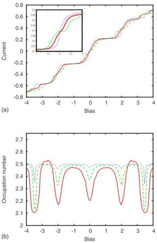
One of the advantages of the Keldysh formalism is that it allows one to investigate the nonlinear transport regime, that is, to study the dependence of the current on the applied bias. We show in Fig.10共a兲the behavior of the current through a T-shaped structure with four side-coupled sites as a function of the applied bias for different values of the interdot
inter-action. The gate potential on the side-coupled sites is fixed to Vg= 0 and also the on-site energy of the contact site is ⑀0
= 0. The bias was varied in a symmetric way as follows: we start with a negative bias V = −4 by choosing ␣= −2 and
= 2. Then, we simultaneously increase the chemical poten-tial of the left lead and decrease the chemical potenpoten-tial of the right lead until the bias changes sign and reaches the final value V = 4.
For U = 0, the current displays the well-known steplike structure. The jumps between two steps correspond to a change in the number of states located inside the bias win-dow. In the absence of the electron-electron interactions, the spectrum of the central region is symmetric with respect to zero. Consequently, the states whose energies differ just by a sign simultaneously align to the positive共negative兲 chemical potential of the leads, and at each passage between current steps, two more states enter or leave the bias window. In the interacting case, one notices the appearance of additional steps 关see, for example, the step around V=2 shown in the inset of Fig. 10共a兲兴. This happens because the Coulomb
in-teraction pushes up the spectrum breaking its symmetry and then two levels cannot enter or leave the bias window
simul-0 0.05 0.1 0.15 0.2 -1.5 -1 -0.5 0 0.5 1 1.5 Current Gate potential 0 0.05 0.1 0.15 0.2 -1.5 -1 -0.5 0 0.5 1 1.5 Current Gate potential (b) (a)
FIG. 8. 共Color online兲 The two-level Fano effect for two T-shaped interferometers. By setting the hopping constant inside the dots to tD= 0.25, two levels can be brought inside the bias window
of the leads by varying the gate potential. 共a兲 Noninteracting case
U = 0.0 and共b兲 interacting case U=0.2. The bias is V=V⬘= 0.2. The full line is the current through the upper interferometer; the dashed line represents the current through the lower interferometer.
0.06 0.08 0.1 0.12 0.14 0.16 -2 -1.5 -1 -0.5 0 0.5 1 1.5 2 C urrent Gate potential 0.8 0.81 0.82 0.83 0.84 0.85 0.86 0.87 0.88 0.89 0.9 -2 -1.5 -1 -0.5 0 0.5 1 1.5 2 C urrent Gate potential (b) (a)
FIG. 9. 共Color online兲 共a兲 The Fano interference in a T-shaped interferometer is further reduced when a nearby charge detector is subjected to a finite bias V⬘. Full line, V⬘= 2; dashed line, V⬘= 1. The dotted line represents the interacting Fano line in the absence of the detector.共b兲 The current across the detector as a function of the gate potential applied on the dot. The charge sensing effect leads to changes in the detector current around each Fano resonance in the side-coupled dot. Other parameters: U = 0.2, V = 0.1, =0.35, and tL= 1.
taneously. Clearly, the length of the steps increases with the interaction strength, a feature that was also noticed by Hen-rickson et al.44共see Fig. 5 of Ref.44兲 within a self-consistent approach to nonlinear transport in interacting quantum dots. Note that the interaction does not affect the symmetry of the current curve with respect to the bias.
The dependence of the occupation number in the dot as a function of bias is shown in Fig. 10共b兲 and offers a better understating of the changes induced in the current curves by the Coulomb interaction. If the bias window covers the entire spectrum of the system, the occupation number N⬃2.5, which corresponds to nearly half-filling. The highest energy level is the first one left above the bias window as the bias window shrinks, while the lowest energy level is still active for transport, as it is being pushed upward by the interaction. In this regime, the occupation number decreases. Then, the lowest level passes below the bias window and it can be fully occupied, which leads to an increase of the charge accumu-lated in the dot and a decrease in the current. Note that when the interaction increases and the bias V = 0, the occupation number goes below 2.5 because the energy of the middle level is positive. We have also checked the current conserva-tion 共i.e., the identity J␣= −J兲. The results presented above
are consistent with previous self-consistent calculations of Henrickson et al.44 and therefore show the reliability of our method. On the other hand, the RPA approach taken here is able to capture nontrivial effects due to the inelastic effects that cannot be reproduced by mean-field approximations.
We end with a discussion about the possible improve-ments of the present method. It is clear that one could per-form self-consistent calculations by defining the polarization operator in terms of interacting Green functions. This proce-dure leads to longer times in the numerical simulations espe-cially for large number of sites. Also, the self-consistency condition should be carefully checked at any value of the relevant parameters 共interaction strength or the tunneling constant between the dot and the lead兲. In the self-consistent scheme, the self-energies will be directly related to the inter-acting Green functions and the position of the poles is ex-pected to be slightly different from the noninteracting case due to the Hartree shift. Nevertheless, for the few-level sys-tem we are considering here, this does not lead to qualitative changes in the numerical results.
IV. CONCLUSIONS
We have implemented the random-phase approximation in the framework of the nonequilibrium Keldysh Green’s function formulation for electronic transport in many-level quantum dots. The starting point is the polarization operator, which in the present approach is built from noninteracting Green functions. The calculation of interaction self-energy takes into account all scattering processes that involve electron-hole pairs and also the contribution of the exchange diagram. This approach has therefore a clear advantage over the second-order perturbation theory in the interaction strength used previously in Ref.27and could also be used as an alternative to the equation-of-motion approach or to the mean-field approximation.
As a first application of this method, we have considered the interplay between the intradot and interdot interactions in electronic transport in Coulomb-coupled T-shaped interfer-ometers. For a single interferometer, the numerical calcula-tions show that the intradot electron-electron interaction it-self suppresses the quantum interference, even in the low bias regime. The various contributions to the interaction self-energy were analyzed as well as the dependence on the bias and gate potential.
In the presence of a second T-shaped interferometer or of a charge detector coupled to leads, further dephasing appears due to the charge sensing effect. We show that the dephasing increases when the Fano interference implies two levels of the dot, which are coupled to the continuum. The high tun-ability of side-coupled quantum dots should allow the obser-vation of our theoretical predictions in future experiments.
ACKNOWLEDGMENTS
V.M. acknowledges financial support by TUBITAK-BIDEB and by CEEX Grant No. D11-45/2005. B.T. is sup-ported by TUBITAK 共Grant No. 106T052兲 and TUBA.
-0.8 -0.6 -0.4 -0.2 0 0.2 0.4 0.6 0.8 -4 -3 -2 -1 0 1 2 3 4 Current Bias 0.2 0.25 0.3 0.35 0.4 0.45 0.5 0.55 0.6 1 1.5 2 2.5 3 2 2.1 2.2 2.3 2.4 2.5 2.6 2.7 -4 -3 -2 -1 0 1 2 3 4 Occupation number Bias (b) (a)
FIG. 10. 共Color online兲 共a兲 Current vs bias for different interac-tion strengths: dotted line, U = 0; full line, U = 0.15; dashed line,
U = 0.25. The interaction leads to the formation of additional steps
when compared to the noninteracting case. The inset shows the formation of a new step in the bias range关1:3兴. 共b兲 The occupation number of the dot as a function of bias for different interaction strengths. Full line, U = 0.15; dashed line, U = 0.05; dotted line, U = 0.01. Other parameters:=1 and tL= 0.5.
1Y. Imry, Introduction to Mesoscopic Physics共Oxford University Press, Oxford, 2002兲.
2Semiconductor Spintronics and Quantum Computation, edited by D. D. Awschalom, D. Loss, and N. Samarth共Springer, Berlin, 2002兲.
3R. I. Shechter, Zh. Eksp. Teor. Fiz. 63, 1410共1972兲 关Sov. Phys. JETP 36, 747共1973兲兴.
4E. Ben-Jacob and Y. Gefen, Phys. Lett. 108A, 289共1985兲. 5D. V. Averin and K. K. Likharev, J. Low Temp. Phys. 62, 345
共1986兲.
6H. van Houten, C. W. J. Beenakker, and A. A. M. Staring, in
Single Charge Tunneling, NATO Advanced Studies Institutes,
Series B: Physics Vol. 294, edited by H. Grabert and M. H. Devoret共Plenum, New York, 1992兲.
7D. Goldhaber-Gordon, H. Shtrikman, D. Mahalu, D. Abusch-Magder, U. Meirav, and M. Kastner, Nature共London兲 391, 156 共1998兲.
8M. Field, C. G. Smith, M. Pepper, D. A. Ritchie, J. E. F. Frost, G. A. C. Jones, and D. G. Hasko, Phys. Rev. Lett. 70, 1311 共1993兲.
9A. C. Johnson, C. M. Marcus, M. P. Hanson, and A. C. Gossard, Phys. Rev. Lett. 93, 106803共2004兲.
10B. L. Altshuler, A. G. Aronov, and D. E. Khmelnitskii, J. Phys. C 15, 7367共1982兲.
11A. Stern, Y. Aharonov, and Y. Imry, Phys. Rev. A 41, 3436 共1990兲.
12S. A. Gurvitz, arXiv:quant-ph/9607029 共unpublished兲; Phys. Rev. B 57, 6602共1998兲.
13E. Buks, R. Schuster, M. Heiblum, D. Mahalu, and V. Umansky, Nature共London兲 391, 871 共1998兲.
14T. Fujisawa, D. G. Austing, Y. Tokura, Y. Hirayama, and S. Tarucha, J. Phys.: Condens. Matter 15, R1395共2003兲. 15U. Sivan, Y. Imry, and A. G. Aronov, Europhys. Lett. 28, 115
共1994兲.
16B. L. Altshuler, Y. Gefen, A. Kamenev, and L. S. Levitov, Phys. Rev. Lett. 78, 2803共1997兲.
17C. Caroli, R. Combescot, P. Nozieres, and D. Saint-James, J. Phys. C 4, 916共1971兲.
18H. Haug and A.-P. Jauho, Quantum Kinetics in Transport and
Optics of Semiconductors共Springer, Berlin, 1996兲.
19M. Wagner, Phys. Rev. B 44, 6104共1991兲. 20D. N. Zubarev, Sov. Phys. Usp. 3, 320共1960兲. 21C. Lacroix, J. Phys. F: Met. Phys. 11, 2389共1981兲.
22V. Kashcheyevs, A. Aharony, and O. Entin-Wohlman, Phys. Rev. B 73, 125338共2006兲.
23Y. Meir, N. S. Wingreen, and P. A. Lee, Phys. Rev. Lett. 66, 3048共1991兲.
24B. R. Bulka and P. Stefanski, Phys. Rev. Lett. 86, 5128共2001兲. 25I. V. Dinu, M. Ţolea, and A. Aldea, Phys. Rev. B 76, 113302
共2007兲.
26A. Silva and S. Levit, Phys. Rev. B 63, 201309共R兲 共2001兲. 27V. Moldoveanu, M. Ţolea, and B. Tanatar, Phys. Rev. B 75,
045309共2007兲.
28J. König, Y. Gefen, and A. Silva, Phys. Rev. Lett. 94, 179701 共2005兲.
29S. V. Faleev and M. I. Stockman, Phys. Rev. B 66, 085318 共2002兲; 62, 16707 共2000兲.
30U. Wulf, P. N. Racec, and E. R. Racec, Phys. Rev. B 75, 075320 共2007兲.
31K. Kobayashi, H. Aikawa, A. Sano, S. Katsumoto, and Y. Iye, Phys. Rev. B 70, 035319共2004兲.
32G. Hackenbroich, W. D. Heiss, and H. A. Weidenmüller, Phys. Rev. Lett. 79, 127共1997兲.
33R. Berkovits, F. von Oppen, and Y. Gefen, Phys. Rev. Lett. 94, 076802共2005兲.
34M. Sato, H. Aikawa, K. Kobayashi, S. Katsumoto, and Y. Iye, Phys. Rev. Lett. 95, 066801共2005兲.
35Tae-Suk Kim and S. Hershfield, Phys. Rev. B 63, 245326 共2001兲.
36R. Franco, M. S. Figueira, and E. V. Anda, Phys. Rev. B 67, 155301共2003兲.
37P. S. Cornaglia and D. R. Grempel, Phys. Rev. B 71, 075305 共2005兲.
38P. A. Orellana, F. Dominguez-Adame, I. Gómez, and M. L. Ladrón de Guevara, Phys. Rev. B 67, 085321共2003兲.
39J. König and Y. Gefen, Phys. Rev. Lett. 86, 3855共2001兲. 40A. Silva and S. Levit, Europhys. Lett. 62, 103共2003兲.
41A.-P. Jauho, N. S. Wingreen, and Y. Meir, Phys. Rev. B 50, 5528 共1994兲.
42H. D. Cornean, H. Neidhardt, and V. A. Zagrebnov, arXiv:0708.3931共unpublished兲.
43V. Moldoveanu, V. Gudmundsson, and A. Manolescu, Phys. Rev. B 76, 085330共2007兲.
44L. E. Henrickson, A. J. Glick, G. W. Bryant, and D. F. Barbe, Phys. Rev. B 50, 4482共1994兲.
45H. M. Pastawski, L. E. F. Foa Torres, and E. Medina, Chem. Phys. 281, 257共2002兲.
46Xin-Zhong Yan and C. S. Ting, Phys. Rev. B 76, 155401共2007兲. 47A. L. Fetter and J. D. Walecka, Quantum Theory of