/S 3 3
1!^» t a ··· l:| и Ч*ЯЦ » i .* л,«, . , ,
“Ч , %· ί» ^ t* * * и1 . (Il* .ш -fc г ^•♦MÄ' 4 l*Ml( Щ 9t lıfifl # *Л. ItAa It * lİL'^ ί ** '*'* *·* Τ !*►*♦>♦ · · · ··* ι ... ■■ " *· ■’■' ’-■ - ^·^ « ■*-· *» * « V ««ιΐ 'Μ/ R Λ α Μи ÏÏ ÎS ; fit; ϊ ftt ж
;i^·'s“!; €: V □ >*«: · } ' « А in· г « - . s ϋ»;4Γΐ..5,.ίϋ Sïi r¿ 2 îU i‘S «а Й “4^I?İîSİİ2Sîi' f|;“
t’!J irr^Äj» ;Ss ;:^ί :Ь ïj ^ ί;^ İ5 ;¿Í ;;|^ -ί;;}·
■ ^ ‘і 'в і Т І г * a 5 W
‘*^‘:aй!д■«г?i^4ад,
'S^ù îf »ί·’IW‘w’'■·
’ ;· : .. J u·!^—i* Λϊ.;,?',tr' ' « - * « ?;ïî ..t·;. Г' ■■ r'"^ >r· ■·: ■: - r « -, ,·, -■ ;,;î·—..-, - - 2Lii’ir' li ν„ι· íi i·,,··.« «,-μ·«·* i;-*S;iftL 2.йУЙ*й-:4‘® i а ϋ'·^.>ΐΤ’ΰ:ίή
*Sî*;l:·-! î:f’::;^TT;f"rÎî:“-f :·' ^ íi'rJM “’“/bíí!ίΓ.'ί::^
**í: Чм:*'і-г^«‘«г t:» Ч-,д -η.,·/ •'»'Ч İHI ·!·4ΐ! V *i ,',ρ' s:, i ■'ïî‘ s ji 2 ' ·* ·■· ^ -.· ·· >·'^ - ·■ '- . ' V- "
::V 3 ..: :r. l··.?:·;, ü: « í í · · ; ; « : ; ï 'Ліз:.·.- : *·' I» IS«' « МЯ «. u i · *í 325^ i *2 - Л! 1'2.V.r''2 ‘i;,.'· ■? ,·, o U : - ' · t:·. i % 4^^íí^r*5í i r r; к З Я Г 2 <·"’Ί ' ■’!C ·■ ''^ '., V T f ' î - ί ’ ΐ Γ ϊ - ί ί · ; ' · v i ‘«i»sï'""îiâr'‘!i|·’ * г·;:... . - ' ..■ . 1-* і" Ж··!·!*:'* Ï 5 «¡ is t; L,<i (ί ν .«·1ιι(1·41 «1 я 4/ V i ' i ÿ , : :î^, ’ - S ' - , :i ;.' · 'W ? “ ІгВШ ТН'£ iíi'i» . . . . и . i » . '■·’■ ! ·-.) ? ·' 1* ? ' . ; - {; í m"ΜW i.i Í«4 ^ ·ι ‘»A" -* M(S i ϋβ ¿1 mît t*,., Н ' Л С і Б · z z Z >ñ. ІЛ.1 ” «· Ι·»· ■ t» '«•.vi !* ■· * 'ii.,-*i."Î.Ï2 '*'2ÿ
GENERAL GRAPHS
A THESIS
SUBMITTED TO THE DEPARTMENT OF INDUSTRIAL ENGINEERING
AND THE INSTITUTE OF ENGINEERING AND SCIENCES OF BILKENT UNIVERSITY
IN PARTIAL FULFILLMENT OF THE REQUIREMENTS FOR THE DEGREE OF
MASTER OF SCIENCE
By
Alper Atamtiirk
December, 1993
è 023230
o ,ç \
ib<o
Assoc. kgul(Principal Advisor)
I certify th at I have read this thesis and that in my opinion it is fully adequate, in scope and in quality, <is a thesis for the degree of Master of Science.
Assoc. Prof. €^man Oğuz
I certify that I have read this thesis and that in my opinion it is fully adequate, in scope and in quality, as a thesis for the degree of Master of Science.
Assoc. Prof. Barbaros Tansel
Approved for the Institute of Engineering and Sciences:
Prof. M ehm et^aray
ABSTRACT
EFFICIENT ALGORITHMS FOR THE MINIMUM COST
PERFECT MATCHING PROBLEM ON GENERAL
GRAPHS
Alper Atamturk
M.S. in Industrial Engineering
Supervisor: Assoc. Prof. Mustafa Akgiil
December, 1993
The minimum cost perfect matching problem is one of the rare combinatorial optimization problems for which polynomial time algorithms exist. Matching algorithms find applications in Postman Problem, Planar Multicommodity Flow
Problem, in heuristics to the well known Traveling Salesman Problem, Vehicle Scheduling Problem, Graph Partitioning Problem, Set Partitioning Problem, in VLSI, et cetera. In this thesis, reviewing the existing primal-dual approaches in
the literature, we present two efficient algorithms for the minimum cost perfect matching problem on general graphs. In both of the algorithms, we achieved drastic reductions in the total number of time consuming operations such as scanning, updating dual variables and reduced costs. Detailed computational analysis on randomly generated graphs has shown the proposed algorithms to be several times faster than other algorithms in the literature. Hence, we conjecture that employment of the new algorithms in the solution methods of above stated important problems would speed them up significantly.
Key words: Minimum Cost Perfect Matching Problem, Primal-dual Algo
rithms, Blossom Algorithm, Fibonacci Heaps.
GENEL ÇİZGELERDE EN KÜÇÜK MALİYETLİ TAM
EŞLEME PROBLEMİ İÇİN ETKİN ALGORİTMALAR
Alper Atamtürk
Endüstri Mühendisliği Bölümü Yüksek Lisans
Tez Yöneticisi: Doç. Dr. Mustafa Akgül
Aralık, 1993
En küçük maliyetli tam eşleme problemi, çözümü için polinom zamanlı algo ritmaların bulunduğu ender kombinatoryal en iyileme problemlerinden biridir. Eşleme algoritmaları Postacı Problemi, Yüzeysel Çoklu Mal Akış Problemi ile iyi bilinen Gezgin Satıcı Problemi, Taşıt Çizelgeleme Problemi, Çizge Parçalama
Problemi, Küme Parçalama Problemi ve diğerleri için sezgisel yordamlarda
kullanılır. Bu tez çalışmasında, literatürdeki primal-dual yaklaşımları gözden geçirdikten sonra, en küçük maliyetli tam eşleme probleminin çözümü için iki etkin algoritma sunuyoruz. Her iki algoritmada da tarama, ikil değişken ve indirgenmiş maliyet güncellemesi gibi zaman alıcı işlemlerin sayısında büyük ölçüde indirime gidilmiştir. Detaylı sayısal analizler önerilen algoritmaların rassal olarak üretilen çizgelerde literatürdeki diğer algoritmalardan birçok kat daha hızlı olduklarını göstermiştir. Sonuç olarak, yeni algoritmaların yukarıda değinilen önemli problemlerin çözüm metodlarında kullanıldığında, bunlarda da kayda değer hızlanmaların olabileceğini söyleyebiliriz.
Anahtar Kelimeler: En Küçük Maliyetli Tam Eşleme Problemi, Primal-
dual Algoritmalar, Gonca Algoritması, Fibonacci Öbekleri.
IV
I am indebted to Associate Professor Mustafa Akgül for his invaluable guid ance, encouragement not only throughout this study but also during my under graduate years. I thank to Associate Professor Osman Oğuz, Associate Pro fessor Barbaros Tansel and Associate Professor Ömer Benli for careful reading of the thesis.
I wish to express my deepest gratitude to my family without whom this study would have not been possible.
I would also like to extend my sincere thanks to Levent Kandiller, for the enthusiasm he inspired on me for the last three years.
My special thanks are to Nilgun Tene for her love, moral support and encouragement.
Contents
1 INTRODUCTION 1.1 P re lim in a rie s ... 2 1.2 Matching P o ly to p e ... 3 1.3 Combinatorial Background 2 LITERATURE REVIEW 122.1 Edmonds’ Blossom A lg o rith m ... 13
2.2 Ball and Derigs’ Algorithm ... 21
3 MULTIPLE AUGMENTATION ALGORITHM 28
4 SINGLE STAGE ALGORITHM 34
5 COMPUTATIONAL STUDIES 41
6 CONCLUSION 50
1.1 A matching example
1.2 A fractional m atching... 4
1.3 A hypomatchable and nonseparable subset of N 1.4 Matching on P before augm entation... 7
1.5 Matching on P after augmentation ... 8
1.6 Shrinking the odd cycle r,x ,y ,z ,s... 9
2.1 Fibonacci H eaps... 15
2.2 G ro w ... 17
2.3 S h r in k ... 18
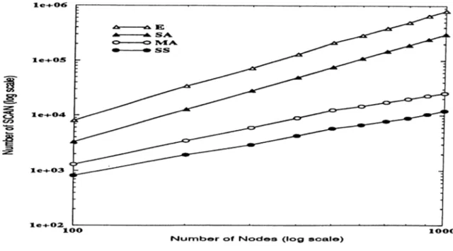
2.4 Expand 19 2.5 Augment 19 3.1 Marking trees, where augmenting paths are found 29 4.1 Heap Elements after an Augmentation 36 5.1 Number of SCAN Operations versus Number of N o d e s ... 44
LIST OF FIGURES vin
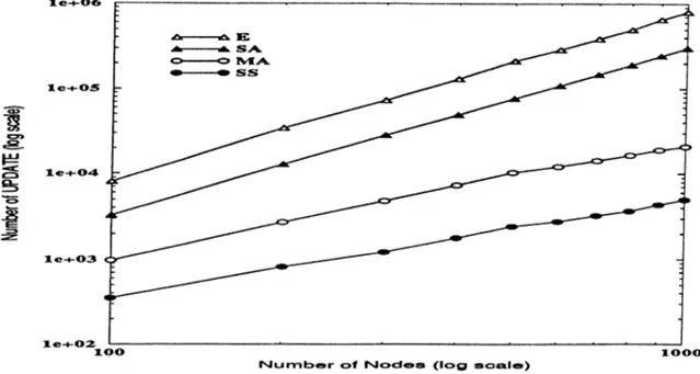
5.2 Number of UPDATE Operations versus Number of Nodes . . . 45
5.3 Number of FINDMIN Operations versus Number of Nodes . . . 46
5.4 Comparison of CPU t i m e s ... 47
5.5 Comparison of CPU times (log-log s c a le )... 47
5.6 Augmentations per Stage versus Ratio of SCAN and UPDATE Operations performed by SA to by M A ... 48
2.1 Worst case complexity of weighted matching algorithm s... 13
5.1 Comparison of SCAN operation by algorithms on random graphs with varying node size, (20% edge d e n sity )... 43
5.2 Comparison of UPDATE operation by algorithms on random
graphs with varying node size, (20% density)... 44
5.3 Comparison of FINDMIN operation by algorithms on random graphs with varying node size, (20% density)... 45
5.4 Comparison of CPU times required by the algorithms on random graphs with varying node size, (20% density)...46
5.5 Comparison of the number of UPDATE operations performed by the algorithms on random graphs with varying edge density, (500 n o d e s ) ... 48
5.6 Comparison of the number of UPDATE operations performed by the algorithms on random graphs with varying edge density, (500 n o d e s ) ... 48
5.7 Comparison of the number of FINDMIN operations performed by the algorithms on random graphs with varying edge density, (500 n o d e s ) ... 49
LIST OF TABLES
5.8 Comparison of CPU times required by the algorithms on random graphs with varying edge density, (500 n o d e s ) ... 49
INTRODUCTION
The minimum cost matching problem is one of the rare combinatorial op timization problems for which polynomial time algorithms exist. Matching algorithms find applications in Postman Problem [10], Planar Multicommodity
Flow Problem [20], in heuristics to the well known Traveling Salesman Prob lem [7], Vehicle Scheduling Problem [4], Graph Partitioning Problem [6], Set Partitioning Problem [21], in VLSI [19], et cetera. In this thesis, we aimed at
finding exact fast algorithms for the problem. We present two such algorithms in the following chapters.
The thesis is organized in six chapters. In the first chapter, we introduce the problem, give the definition of the matching polytope and present augmenting paths for finding matchings on graphs. Second chapter reviews two important primal-dual algorithms for the problem. In chapters three and four, we give two efficient algorithms, respectively. A series of detailed computational studies is summarized in chapter five. Finally, we conclude the presentation with chapter six.
1.1
P r e lim in a r ie s
Let G = {N, E) be an undirected graph, where N is the set of nodes, E is the set of edges and c be a real valued cost vector associated with the edges. We will use n to denote the number of nodes and m for the number of edges of graph G. A matching M on G is a subset of edges no two of which are incident to a common node. An edge in M is called a matching edge·, conversely, every edge not in Af is a free edge. A node is said to be a matched node if it is incident to a matching edge and a free node otherwise. The size of M is the number of edges it contains and the cost of M is the sum of its edge costs. A
perfect matching has size n / 2. The problem we want to solve is that of finding
a minimum cost matching among the perfect matchings on G.
CHAPTER 1. INTRODUCTION 2
D
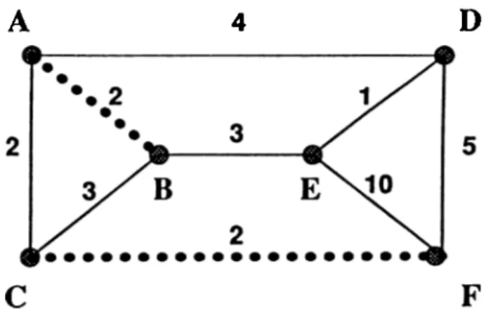
Figure 1.1: A matching example
In Figure 1.1 a matching on a small graph is illustrated. Dotted edges, (A,B) and (C,F) represent the matching edges. Rest of the edges are free. Only nodes E and D are free, others are matched nodes. Obviously, matching
1.2
M a tc h in g P o ly t o p e
Let Y C N ,
A(K) = e E : i € Y, j i Y)
r ( n = { { i j ) e E i i e Y J € Y}
We may simply refer to A (F ) as the cut edges of Y . S(Y) G /2*” is a vector associated with the edge set A (F ), where component of S{Y) is 1 if edge is in A (F ), 0 otherwise. We also define 7 (F ) € R”^ similarly for the set r ( F ) . If F is a singleton we simply write ^(t) instead of and A(i) for A({i}). Furthermore let us define the incidence vector G /2”* of F C E, where component of is 1 if A:‘* edge is in F, 0 otherwise.
Let 'Pjv^(G) be the perfect matching polytope of G, which is the convex hull of the incidence vectors of perfect matchings in G, i.e.
Fm{G) = conv{x^ G /2”* : Af is a perfect matching in G)
Using combinatorial properties of the problem, Pm(G) is described with a set
of linear equalities and inequalities.
First, let X be an integer vector to describe a matching, then, the minimum
cost perfect matching problem can be formulated cis:
min s.t.: T c X P I) x'^S{i) = 1 , V i G AT X 6 {O,!}”»"*
The equalities used in PI are called the assignment equalities and when x is a binary vector, they indicate that for every node in the graph only a single edge incident to it should be in the matching. However, with this integer formulation it is very unlikely to solve the problem in polynomial time, unless P = NP. On the other hand, linear programming (LP) relaxation of PI does not guarantee an integer solution for the problem. Mere the assignment equalities in this case may yield a fractional solution. This is easy to see in Figure 1.2.
= (0,0,0,0.5,0.5,0.5,0.5,0.5,0.5) is an extreme solution of the LP relaxation of PI.
CHAPTER 1. INTRODUCTION 4
x, = 0
D
D efin itio n 1.1 For G = {N ,E ) and W d N we define G[W] = (lP ,r(l'P ))
and call it subgraph induced by W.
D efin itio n 1.2 A cutnode of a graph G — (N ,E ) is a node w E N such that
G[N \ {tw}] has more connected components than G has.
D efin itio n 1.3 y4 graph G is called nonseparable if it does not contain any
cutnode.
D efin itio n 1.4 For an odd cardinality W C G with |H^| > 3, G\W] is called
hypomatchable if for every w there exists a perfect matching with respect
to G [fr\{ u ;} ].
For X € R!J! and every IV C N with |VF| > 3 and odd, the following
inequality is valid for Pm(G) :
This type of inequalities are called blossom inequalities and are due to Ed monds [9]. Edmonds has shown that together with the assignment inequalities, they describe Vm- Even though sufficient, they are far from being minimal.
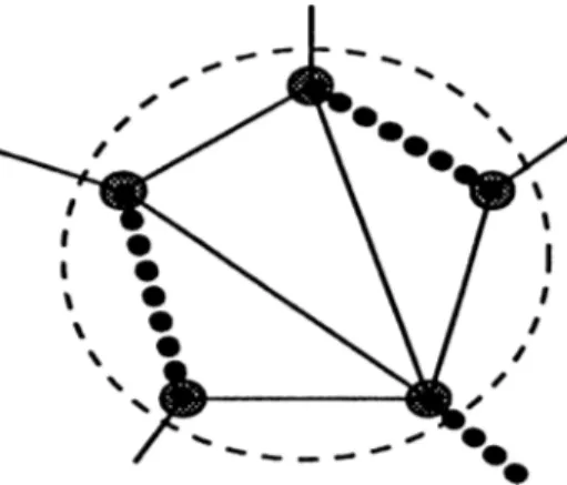
T h e o re m 1.1 (E d m o n d s a n d P u lle y b la n k [10]) Hyperplanes represented by
the blossom inequalities fo r odd cardinality W C. N with | IE |> 3 are the facets
o f Vm If only if G[VE] are hypomatchable and nonseparable (Figure 1.3).
Figure 1.3: A hypomatchable and nonseparable subset of N
Let us use Q to denote the set of all such facet defining subsets of N . Then, facet defining blossom inequalities with the assignment equalities, lead to the below given blossom characterization of the minimum cost perfect matching
problem, mm s.t.: T c X P2) = i y i e N x ' ^ i { W ) < [ \ ! 2 \ w \ \ y w e Q x > Q
Similarly, for IE G Q , we also have the following cut inequalities,
CHAPTER 1. INTRODUCTION
to represent facets of Vm· Using the cut inequalities we can re-formulate
the problem. min c^x s.t.: P3) = 1 V i e N x'^6{W) > 1 v w e Q X > 0
The above formulation is called the cut characterization. Actually there is a bijective linear transformation between the two characterizations.
The dual problem of P3 is,
max s.t.:
12içN Vi + ICweQ yw
D3) y.·+ y i + E{yiv :(*■,;) e A(iU)} < C.J ' i { i , j ) e E yw > 0 V VP € g Let Cij denote the reduced cost of an edge ( i,j) € E., i.e.
Cij = Cij - Vi - y j - 53{yw : (*,i) € A(VP)}
Then the complementary slackness conditions of the linear program for a given
M can be stated as,
( t,i) € M ^ Cij - 0
y w > 0 = ^ |M nA (V P)| = 1
Even though linear characterization of the problem bears exponentially many inequalities in the number of nodes, importance of it comes from the fact that resulting complementary slackness conditions become very powerful tools in designing efficient algorithms for the problem. Also the combinatorial properties of the problem provides enough information so that only O(n^) of the inequalities are encountered in solving the problem.
1.3
C o m b in a to r ia l B a c k g r o u n d
D efin itio n 1.5 A walk on G is a finite sequence o f nodes and edges, where
the elements of the sequence are altematingly a node and an edge and where the starting and ending elements are nodes of G. A path on G is defined as a walk in which all nodes are distinct.
Even though a path is a sequence, we do not distinguish the sequence and the set of elements in the sequence since it will not cause ambiguity in our context.
D efin itio n 1.6 An alternating path is a path where edges are alternatingly
matching and free.
D efin itio n 1.7 An augmenting path is an alternating path whose both ends
are free nodes.
Augmenting paths play a crucial role in matchings. An augmenting path is found by growing alternating paths; whenever one is found, the cardinality of the matching can be increased simply by swapping the free edges and the matched edges on the augmenting path. This is said to be an augmentation. In figure 1.4 an example augmenting path is given. The new matching on the same path after an augmentation is shown in figure 1.5. Thus if M is augmented by the augmenting path P, the new matching M is
A7= A /A P
where M A P denotes the symmetric difference operation on sets M and P.
Figure 1.4: Matching on P before augmentation
Next theorem is used as a stopping criterion in finding maximum cardinality matching.
CHAPTER 1. INTRODUCTION
Figure 1.5: Matching on P after augmentation
T h e o re m 1.2 (Berge[5]) A matching M in G contains the maximum number
of edges if and only if it admits no augmenting path.
D efin itio n 1.8 Let M be a matching in G and let P be an alternating path
with respect to M . We define the length of P as:
4 P ) = IZ Z )
{ i , j } € P n M
Similarly reduced cost length of P is defined as:
^{P)=
Z
Z
{ • j } e P W { i j J e P n M
L em m a 1.1 Let P denote an augmenting path with respect to M in G, then
cost of the augmented matching M , accounts to
Z_^i= Z
+
P ro o f : This holds true, by definitions of C{P) and M .
Hence, cost of the matching is increased by the length of the augmenting path after an augmentation. Now suppose we have have a matching A/*, with I M* 1= k and c{M*) is minimum among all matchings of cardinality k. Then from Lemma 1.1 a, minimum length augmenting path with respect to M* will lead to M with \ M |= A: + 1 and c(M ) minimum among all matchings of cardinality k. Lemma is also valid for the case A/ = 0 for which minimum length augmenting path is simply an edge with minimum cost. So the problem boils down to successively finding minimum length (shortest) augmenting paths between pairs of free nodes until every node is matched. This solution method is called the shortest augmenting path method.
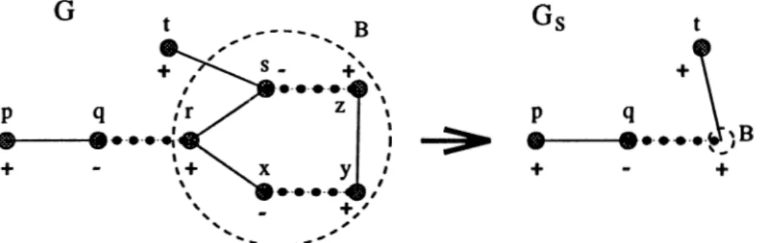
This method of growing alternating trees is performed with ease if the graph is bipartite. However there is a complication in non-bipartite graphs : odd cycles. In figure 1.6 a walk on nodes p, q, r, s, t does not lead to an augmenting path, however there is actually an augmenting path between p and t, which is the walk on p ,q ,r ,x ,y ,z ,s ,t . Existence of odd cycles such as r , x , y , z , s bring about a major difficulty in the identification of augmenting paths. This difficulty is overcome by shrinking the odd cycle into a pseudonode say B . In the same figure it is clear that after the shrinking operation the augmenting path can easily be found.
Figure 1.6: Shrinking the odd cycle r,x,y,z,s
D efinition 1.9 Given G = (N ,E ) let W be a subset of N forming an odd
cycle. Gs = {{N \ W ) U B , { E \ r(VF))), where B is a pseudonode (blossom) obtained by shrinking W , is called the surface graph.
Note that blossoms can be nested, that is a pseudonode and some other (pseudo)nodes in Gs can further be shrunk to form another blossom. In this case, the new surface graph is obtained similarly. If we call the elements that are most recently shrunk in a nested blossom B as maximal., through expan
sion of B one can retrieve those maximal elements of the nested blossom B.
Each one of the maximal elements may be a blossom or a node in G. Let il denote those maximal elements of B. If G$ = {Ny E) is the surface graph be fore the expansion of B, the new surface graph obtained after expansion will be
CHAPTER 1. INTRODUCTION 10
Since minimum number of maximal elements in a blossom is three, maximum number of blossom formation is n /2 — 1. This observation will justify that a polynomial number of the blossom (or cut) inequalities in P2(P3) become tight. Shrinking and expanding blossoms will be explained in detail in the following chapter.
L em m a 1.2 Let Ps be an augmenting path found in Gs· Ps induces an aug
menting path P in G.
P r o o f ; The lemma directly falls from the fact that the blossoms on Ps are hy- pomatchable and nonseparable. Recursive expansion of the maximal elements of the blossoms on Ps leads to P.
At this point we will relate the augmenting paths to the generic primal dual algorithm. It is possible to view shortest augmenting method as in instance of the generic primal dual algorithm. Given a feasible dual solution y (possibly y = 0) to D3 let us call EG{y) = {N, E{y)) equality subgraph, where
E{y) = {e
e E
: Ce =0}
Furthermore let matching M in EG{y) that satisfying the complementary slackness conditions be a compatible pair of y. If M is perfect, that is the primal problem also feasible, then it is optimal. However if M is not perfect, from theorem of alternatives, there exist a feasible direction d, strictly speaking a ray in the dual cone for EG{y), that is the graph restricted to the edges in
E{y). So we can improve the dual solution in the direction of the ray. The
amount of improvement is however dictated by an edge in \ E{y). Let 6 be the maximum improvement in the direction d without violating dual feasibility for the edges in \ E(y), then
0 = min{ce : e e E \ E{y)}
Now an edge e' with Ce< = 0 will be in the new equality subgraph EG{y') =
{N, E[y')), where y' — y-\-0d. Hence maintaining the complementary slackness
optimal or improve the dual objective function. Equality subgraph helps us to maintain the basic invariant of the generic primal dual algorithm, that is the satisfaction of the complementary slackness conditions.
In the shortest augmenting path method, edges on the alternating paths are part of the equality subgraph. Search for an edge with minimum reduced cost to grow a path is nothing but a ratio test of reduced cost among the edges not in the equality subgraph. Growing an alternating path amounts to improving the dual solution. Hence the method is just a combinatorial instance of the generic primal dual algorithm.
Expansion of blossoms turns out to be one of the most cumbersome op erations in matching algorithms for non-bipartite graphs impeding both theo retical and practical computational efficiency. In bipartite graphs, expansion and shrinking are not needed since from an combinatorial point of view, odd cycles are not encountered and from a linear programming point of view, all the variables of the dual problem are free.
Chapter 2
LITERATURE REVIEW
Edmonds[9] presented the first efficient algorithm of O(n^) for the matching problem, which can easily be implemented with O(n^m) complexity. After wards, there came several other primal-dual algorithms, that are improvements of Edmonds’ blossom algorithm. Gabow[13] and Lawler[18] have independently shown that blossom algorithm can be implemented with O(n^) complexity. Galil, Micali and Gabow[16] gave an O (nm logn) algorithm using splittable
heaps. Ball and Derigs[3] presented O(n^) and O (nm logn) algorithms that
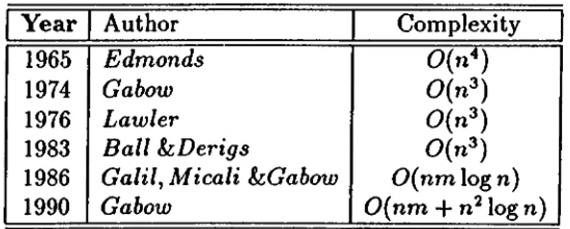
are modifications of the previous ones. Essentially, decrease to 0(nm log n) is achieved through utilization of elegant data structures, rather than a change in the main algorithm. Gabow has recently given an 0 (n m -|- log n) algo rithm for the problem, which also uses quite complicated data structures [14]. There exist other solution methods for the problem such as, primal [8], scaling [15] and cutting plane [17] algorithms; however, here we will concentrate on primal-dual algorithms. Table 1 lists the primal dual algorithms known to us for the minimum cost perfect matching problem.
In the following two sections we will describe our implementations of Ed
monds^ Blossom Algorithm and Ball & Derigs’ Algorithm, respectively. These
implementations are somewhat different than they were originally described. Firstly, our implementations allow growing of many alternating trees simulta neously, rather than one at a time. Secondly, we employ state-of-the-art data
Y ear Author Complexity
1965 Edmonds O K )
1974 Gabow 0(n^)
1976 Lawler O(n^)
1983 Ball L·Derigs O(n^)
1986 Gain, Micali hGabow 0 (nm log n)
1990 Gabow 0 (nm + log n)
Table 2.1: Worst case complexity of weighted matching algorithms
structures such as Fibonacci Heaps which were not known at the time these algorithms were first posed.
2.1
E d m o n d s ’ B lo s s o m A lg o r ith m
We grow alternating trees rooted at each free node to find augmenting paths between pairs of free nodes. The collection of such alternating trees will be called the Planted Forest, PF. Initially, P F consists of trivial trees of single free nodes with © labels. As the trees are grown larger, nodes will assume labels ©/© alternatingly. After an augmentation, trees rooted at newly matched nodes are moved to the Matched Forest, M F , where they are labelled 0. In the case an odd cycle is encountered, it is shrunk to form a pseudonode. As defined in the previous chapter, this new graph induced by the shrinking operation is called the Surface Graph, Gs· From now on, every node in Gs will be called a
blossom. Thus some blossoms are trivial and exist in G = (A^, E), as well. Let
us use b{j) to denote the blossom in G$ that node j is in. In referring to all the nodes j G: N that are included in b{j), we will say real nodes of b{j) and denote them as Real(b(j)).
The Blossom Algorithm aims to find an augmenting path between a pair of free nodes at each iteration. The search for a minimum cost augmenting path is realized by growing minimum reduced cost alternating paths on Gs· Actually, all of the trees rooted at a free node are grown simultaneously, so the
CHAPTER 2. LITERATURE REVIEW 14
augmenting path can be found between any of the trees. When an augmenting path lying on two such trees is found, that is when a minimum cost augmenting path between any two of the roots of the trees in P F is detected, the path is augmented and both of the trees on which the augmenting path lies are carried to M F . After this, a new iteration starts to search for another augmenting path on the remaining alternating trees in PF.
Within an iteration, search for an augmenting path is pursued by seven basic operations. These are Scan, Update, Findmin, Grow, Shrink, Expand and Augment These operations basically have the same function in all of the algorithms that will be presented here, however there exist slight modifications from algorithm to algorithm. At this point, we present the pseudocode of the main algorithm. Then we will describe each operation in detail.
E d m on ds’ B lossom A lgorithm w hile PF Ih do begin Scan(A:),Vfc 6 PF; Update(A:); VA: € PF ( c ,b i) ^ FindminO; if(6 = Cyi) G row (i,i); if (t = 6b)
begin
if (i and j belong to the same tree)
Shrink(t,j); else A u g m en t(t,j); end if (c = ec) Expand(i); end R ecover(M F);
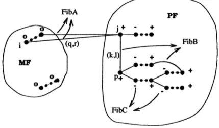
We utilize three Fibonacci Heaps [12] to facilitate fast Findm in operation. Findmin outputs the minimum key (c) over all the three heaps. FihA is for the edges which have one end in M F and one in a © labelled blossom. FihB is for edges with both ends in different © labelled blossoms and FibC is for keeping the dual variables of 0 labelled non-trivial blossoms in PF. For each blossom i in M F we have an element in FibA that keeps the minimum reduced edge from t to a © labelled blossom in PF. FibA; denotes the key in FibA for
the minimum reduced cost cut edge (q, r) of i in figure 2.1, such that b{q) = t,
6(r) = j and Ibi = 0, Ibj = 0 , where /6,· denotes the label of i. In order to store
this edge, we have two entries associated with the heap element, node to keep
q and nb (neighbor) to keep r. Key is the reduced cost of edge (q, r) denoted
as Cgr. FibBj is the key in FibB for the minimum reduced cost edge from 0 labelled blossom j to another 0 labelled blossom. FibBj is half of Cki oí the co-boundary edge (ky 1) of j in the same figure, such that b(k) = j , b(l) = p and Ibj = Ibp = 0 . It is possible that both j and p have distinct elements in
FibB for the same edge. If such an edge causes an augmentation, we simply
delete both of the relevant elements from FibB. Finally, each non-trivial 0 labelled blossom in P F has an element in FibC with a key FibCi that is equal to dual variable of i. In FibC, nb entries are empty since it is for dual variable information of blossoms, rather than for reduced cost of edges.
Figure 2.1: Fibonacci Heaps
In Edmonds’ algorithm Scan is called at every iteration. By scanning each element in the cut edges of 0 labelled blossoms in PF, the minimum reduced cost edge (kept in Fib/[ with the key being the reduced cost) from each 0 labelled blossom to a 0 labelled blossom and the minimum reduced cost edge (kept in FibB with the key being half of the reduced cost) from each 0 labelled blossom to another 0 labelled blossom are determined. Dual variables of 0 labelled blossoms are stored in Fibc·
CHAPTER 2. LITERATURE REVIEW 16 Scan(t) begin if (Ibi = ©) then for V()b, j ) e A ( t ) : b(k) = i do begin if = 0) then FibAk(j) 4- min{FibAk(j),Ckj)\ if = 0 ) and {b{j) ^ t) then FibB(,Q) 4- min{FibB^j^,0.5ckj}; end
else if (Ibi = ©) and (i ^ N) th en /* i is a pseudonode */
FibCi 4- y, ; end /* Scan */ Findm in() begin €a ^ min,'{Fi6i4,·}; €b min,{Fi6B,·}; €c ^ min,{Fi6C,·}; 6 ^ min{6yi,6B,cc};
q <— node achieving this minimum; i 4- b{q);
j 4- b{nbi);
end /* Findmin */
After Scan, Findmin is called to find the minimum key over all of the three heaps, e is this minimum key and q is the real node achieving this minimum.
Now that e is known, Update is called to change the dual variables of the blossoms and the reduced costs of edges in Gs- For each 0 labelled blossom t,
yi is increased by e while reduced costs of the cut edges of i are decreased by e.
Conversely, for each 0 labelled blossom i, yi is reduced by e while reduced costs of the cut edges are increased by e. Observe that, with this kind of an Update operation dual feasibility is maintained for every edge and reduced costs of the forest edges (edges in the equality subgraph) are kept zero. Reason for keeping only half of the reduced cost of edges between different © labelled blossoms in FibB should be clear now. If c = cb with cb = 0.5ce, after the update
Ce becomes zero since e is deducted for both of the 0 labelled blossoms the end nodes of e are in. Also note that at each iteration dual objective function
U pdate(t) begin if (Ibi = ©) then begin Vi ^ Vi
+ c;
for (k,j) G A ( t ) : b(k) — i do ^kj ^ ^kj end else if (Ibi = ©) th en begin Vi Vi -c;
for (k,j) 6 A(t) : b(k) = i do C kj * - C kj + €] end end /* Update */improves as much as (| | —2 | M |) c. This claim follows from the fact that there are (| | —2 | M |) more 0 labelled blossoms than 0 labelled ones in
PF. mate(i) Figure 2.2: Grow Grow(j, i) begin parenti <— j; parent^^teii) ^ »; Ibi
0;
^^mote(i) ^ end /* Grow */Grow is called if Findmin outputs an edge between a 0 labelled blossom j
and a 0 labelled blossom i. In this case, i is made a child of j and moved to
P F from M F together with its matched blossom, denoted as mate(i). Please
refer to fig 2.2.
CHAPTER 2. LITERATURE REVIEW 18
i and j on the same alternating tree. This is the case, when an odd cycle is
found. The odd cycle is shrunk to form a new 0 labelled blossom. Nearest
common ancestor oi i and j , denoted as nca{i,j), is the first common blossom
of paths from i and j to the root of the tree. In figure 2.3 let Pi be the path from i to n ca(t,j) and Pj be the path from j to nca{i,j).
Shrink(i, j ) begin
Shrink P i U P j U (i,j) into B ;
Update Gs",
V B 0;
lbs *—®;
end /* Shrink */
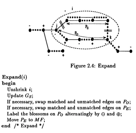
Expand is called if Findmin outputs a non-trivial 0 labelled blossom t. In
this case, i is expanded and Gs is updated to include the maximal elements in
i. Please refer to figure 2.4 for this operation. Let j be the maximal element in i where the unmatched edge in A (i) emanates from, and let k be the maximal
element in i where the matched edge in A(i) emanates from. Furthermore define Pq as the path between j and k with odd number of blossoms, including
j and k. and Pe as the path between the remaining blossoms of i. Existence of
Po and Pe is guaranteed since there are odd number of maximal elements in
i. Note that primal feasibility may be violated for the edges on the alternating
path between maximal elements. This can be reconstructed simply by swap ping the matching edges and free edges on one of the paths. Since swapping takes place in the equality subgraph the objective function is not affected.
0·#·· ^ ^ ^ ^ A • r ^ 1 . Pe ...* ·^ • *’·... . f • t - — 0 e e e e 4 i — ♦ ♦ Figure 2.4: Expand Expand(i) begin Unshrink t; Update Gs]
If necessary, swap matched and unmatched edges on Pq]
If necessary, swap matched and unmatched edges on Pe‘,
Label the blossoms on Pq aJternatingly by 0 and 0 ; Move Pe to MF·,
end /* Expand */
Augment is called if Findmin outputs an edge between two 0 labelled blos
soms i and j on different alternating trees, denoted as T, and Tj respectively in figure 2.5. This is the case, when an augmenting path between the roots of the trees is found. Now, define f*,· as the path from i to the root of Ti and Pj from j to the root of Tj. Then the augmenting path is P = P,· U {i,j) U Pj.
After all the nodes are matched Recover is called to expand all the nested blossoms. One may refer to figure 2.4 again for this operation. Let j be the
CHAPTER 2. LITERATURE REVIEW 20
A ugm ent(i,j)
Swap matched and unmatched edges on P;
Ti ^ Ti \ Pi ; T'i ^ T j \ Pi·,
Move P, T[ and Tj to MF; end /* Augment */
blossom in i where the unmatched edge in A(t) emanates from, and let k be the blossom in i where the matched edge in A(t) emanates from. Furthermore define Po as the path between j and k with odd number of blossoms, including
j and fc, and Pe as the path between the remaining blossoms of i. Finally, let
L be the list of maximal elements in i. Recover is very similar to expand; it
may be viewed as recursive expand operation. Recover(i) if i 6 A return; else begin Unshrink i; Update Gs',
Swap matched and unmatched edges on Pq such that
j is adjacent to a matched edge on Po‘,
Swap matched and unmatched edges on Pe such that
blossom adjacent to j is adjacent to a matched edge on Pe‘,
Recover(/) ,V/ € L; end
end /* Recover */
The algorithm performs Scan and i/pdaie operations before one of the Grow,
Shrink, Augment or Expand operations is called. Scanning and updating before
such a call can be done in 0{m ) time. The other operations can easily be performed in 0 (n ). Between two augmentations there are 0{n) iterations, so the work needed to be done between augmentations is 0{nm ). Since there is a total of n /2 augmentations, we have O(n^m) complexity for the blossom algorithm.
2 .2
B a ll a n d D e r ig s ’ A lg o r ith m
In this section, we define a new terminology called stage. A stage is the period between two augmentations, so it consists of a series of iterations, which ends with an Augment operation. Lawler showed the possibility of implementing the blossom algorithm in such a way that an edge is scanned at most two times during a stage instead twice at each iteration. The basic observation here is that as long as label of a blossom remains the same, its dual variable will continue either to increase or to decrease depending on its label. Change in the reduced cost of the cut edges of that blossom will be in the reverse direction. Within a stage, if the aggregate amount of change that should be done in the dual variable of blossoms and in the reduced costs of the cut edges can be maintained in an efficient way, it may be possible to use this information to arrive at the actual dual variables and reduced costs without the need to calculate them at each iteration. Hence, computational complexity will be reduced to O(n^) and one will achieve considerable saving in the total number of the Scan and Update operations between augmentations.
In this algorithm scanning of a cut edge is done only when blossom of one of the end nodes of the edge assumes a 0 label in a stage. Observe that once the blossom of a node assumes 0 label in P F it will remain © till the end of the stage. Thus an edge is scanned at most twice throughout a stage. However there exists a bit difficulty with © labelled blossoms, since blossom of a real node that was previously © labelled may assume 0 and © labels through successive expand and grow operations. Tackling © labelled blossoms will be explained further in detail.
The algorithm of Ball L· Derigs[3] which is an improvement of Lawler’s orig inal algorithm performs the same Findmin, Recover and similar Grow, Shrink,
Augment, and Expand operations cis Edmonds’. Improvement is achieved
through modification of the main algorithm and of Scan and Update opera tions. The algorithm has two loops, inner and outer. Each call of the outer loop is a stage and there is a total of n/2 stages throughout the algorithm.
CHAPTER 2. LITERATURE REVIEW 22
Ball &; D erigs’ Algorithm while FF ^ 0 do begin Scan(A:),VA: 6 PF; repeat ^ FindminO; if (€ = (a) Grow (t,;); begin
if (t and j belong to the same tree) Shrink(t, j);
else Augment(i, j); end
if (e = (c) Expand(i);
until [there is an augmentation) Update(fc); VJk G PF
Full_Update(); end
Recover(M F);
For delaying the Scan and Update operations, we have a variable d,· for each blossom i in P F . di keeps the value of e when blossom i is moved to the P F during a stage. Rather than updating dual variables and reduced costs at each iteration of the algorithm, amount of update needed is stored in such a way that actual update can be performed at the end of a stage. The amount of update to be done for the dual variable of a blossom i in P F that existed in
Gs at the beginning of a stage and for the reduced cost of the edges in A[i)
is equal to c — at any time in the stage. This amount may be viewed as a measure of presence of blossom i in P F during the stage.
Grow(i, j) begin parenti *— j ; p a r e n t ^ a t e ( i ) Ibi ©; di <- e; end /* Grow */
cost updates of the cut edges of 0 labelled blossoms. When a 0 labelled pseudonode is expanded, reduced cost update for some cut edges will be in the reverse direction since the real nodes these edges emanate will now have a 0 labelled blossom in the new surface graph instead of a 0 labelled one. We will decrease the reduced cost of these edges, which we used to increase before the expansion. Updating the reduced cost of these edges during expand will give an 0 (n m ) complexity for a stage, since we may have to update same edges over an over again as a nested 0 labelled blossom is expanded recursively during a stage. To overcome this difficulty, relevant updates are performed on the realnodes. For this, we utilize w array of size 0(n). Amount of update needed to be done on the reduced costs of these edges are kept in the entries of w for the real nodes that the edges emanate from, w array will also be utilized
in the
Shrinkoperation. Necessary reduced
costupdates
for the cutedges
ofblossoms that are shrunk into a new pseudonode will be kept in the entries of
LUr Total work for updating elenientH of t u ¡3 of O(n^) roiiijiloxity throughout a
stage, since both of the shrink and expand can be called 0 (n) times per stage.
Expand(t) begin
Unshrink i; Update Gs;
If necessary, swap matched and unmatched edges on
PolI f nocGsisary, s w a p n i a t c h o d a n d u n m a t c h e d e d g e s o n L a b e l t h e b l o s s o m s o n a l t e r n a t i n g l y b y © a n d m i dj € VJ o n Po\ Wr tCr + (e - d{) Vr e Real{i);
Move
P
eto
MF\
end /* Expand */Recall that during an expansion matched pairs of blossoms may be carried
t o M b \ T h iN h r i i i g s n e w e d g e s In d .w e e n F F a n d M F w h i c h a r e n o t s c a n n e d
before. If we were to scan these edges and put the minimum reduced cost
edge from a new blossom in MF to a 0 labelled blossom, in FiM, complexity
of a stage becomes 0{nm ) again. This is due to the fact that we may have to scan some of these edges over and over again (at most 0 (n ) times) as nested 0 labelled blossoms are expanded recursively during a stage. To solve this problem, Lawler’s idea was to keep the reduced costs of edges between 0
CHAPTER 2. LITERATURE REVIEW 24 Shrink(i, j) begin for VA: on Pi U Pj do begin if Ibj — 0 then yfc i/fe + (f - dik);
for Vr 6 Real(k) *— — {e — djt);
else if Ibj = 0 then
Vk Vk - ((+ dk);
for Vr € Real{k) Wr + (f — dk)\ end
for VA: on Pi U Pj do if Ibk = 0 then Scan(A:); Shrink Pi U Pj U (t, j) € E into B] Update Gs]
VB 0;
lbs <— 0 ;
end /* Shrink */
labelled blossoms and 0 /0 labelled blossoms in an array. Let p and v be two
0 {n ) arrays and entry of p, pj be the other end of an edge from the real
node y to a 0 labelled blossom with minimum reduced cost. Vj is the reduced cost of this edge as at the beginning of a stage. When a blossom bo is moved to
M F after an Expand operation, a search is done on Vj for every real node of bo
and a new key is inserted to FibA for a minimum reduced cost edge from bo to a 0 labelled blossom. This is just an 0 (n ) work for each expand. Utilization of these two arrays makes it possible to scan a 0 labelled blossom only once throughout a stage, hence brings about considerable saving in the number of
Scan operation.
The Scan operation in this algorithm not only computes the keys of the Fibonacci Heaps but also the entries of the v and p arrays. A blossom 6® is scanned only when it first time assumes a 0 label in a stage, so db^ = e. We call the cut edges of b^ to 0 and 0 labelled blossoms as candidate edges. Let us first consider the reduced cost of an edge (j, i) between a 0 labelled blossom bo and 0 labelled blossom 6®. Observe that at any time during the stage updated amount of Cj·,·, which we will denote as Cji equals to Cji-{e — db^) + Wj-\-Wi, since (e — + + is the amount of reduction we have delayed to perform on c_,,·.
In this sum (e — ) term reflects the delayed update after 6® first appeared in
P F , while Wj + Wi is for any update at a shrink and/or expand operation before
the appearance of 6®. Recall that w array is for complementing reduced cost updates for which (j, i) used to be a co-boundary edge of a blossom disappeared from the surface graph through a shrink or an expand operation. For the real nodes of j of bo a candidate edge heis cjk = cjk + wj + u?jt, so it is valid to compare the value cjk + wj for candidate edge (j, k) with vj — (e — db^) + Wp. since Vj assumes the value of Cjp- at the beginning of stage, where {j,Pj) is the edge with minimum reduced cost value from / to a 0 labelled blossom.
Now, let us look at the situation for reduced cost of an edge (/, k) between a 0 labelled blossom 69 and a 0 labelled blossom 6®. Updated reduced cost
Cjk is equal to Cjk — (c — ¿6®) + (c “ <^69) + + ^fc· For real nodes of j of 69,
a candidate edge {j, k) has cjk equal to cjk + (e — db^) -|- wj + Wk. That is the justifying reason of comparing Vj — (c — ¿6®) + Wp^ with cjk + Wk. In order to maintain the order relationship among the elements of heaps, e is added to its actual key value of a new element when it is inserted to one of them. This is necessary since keys in the heaps are not updated at each iteration.
Scan(i) begin
if (/6,· = ©) th en
for V(Ar, j) G A(t) : b(k) = i do begin if = 0) th en FibAb(j) <- min{FibAb(j),Ckj -|- Wk -|- Wj -|- f}; if = ©) and (b(j) ^ i) th en FibBb(j) min{FibBb(j),0.!j{ckj - {e - dj) + Wk -|- -|- c}; if ( Ckj + Wk< Vj - { ( - db(p^)) -I- Wp^) then Vj c/fj·; Pi ^ k; end
else if (/6,· = 0 ) and (i ^ N) then
FibCi *- Vi + t;
end /* Scan */
As stated above, amount of update to be done for dual variable of blossom
CHAPTER 2. LITERATURE REVIEW 26 U p d a te(t) begin if (/6,· = 0 ) th en begin Vi Vi + ( e - di)·, for (k, j ) € A ( i ) : b(k) = t do ^kj * ^kj “ (f ~ ^t)i end e lse if (Ibi = 0 ) th en begin Vi < - Vi - ( c - di)] for (k, j) G A ( t ) : b{k) = i do Ckj Ckj + (f - dj); end end /* Update */
algorithm is modified to allow a cumulative increase or decrease depending on the label of blossom i.
At the end of a stage Full. Update is called to complement the updates on the reduced cost of the edges which we have delayed at Shrink and Expand operations throughout the stage. With this operation all of the delayed updates on the reduced cost of every edge are completed for the stage.
F u lL U pdate() begin
C i j C i j + W i + W j V(i, j) G E]
end /* Full_update */
During a stage an edge is scanned at most two times, that is when blossom of its end nodes assume 0 label, which gives 0 (m) for total scanning operations. All of the other operations in an iteration is bounded with 0 (n ) time . Since each of the operations can at most be called 0 (n) times between augmentations, complexity of a stage becomes O(n^). Thus, the overall complexity of the algorithm is O(n^). Instead of v array, if we were to keep a splittable heap for each 0 and 0 labelled blossom, we could complete an expand operation in O(log n) time. When a 0 labelled blossom is expanded, its heap, which stores the minimum reduced cost to a 0 labelled blossom, is split to form other heaps for each of the maximal elements of that blossom that eissumes a 0 or 0 label
at the new surface graph 0(log n) time. However in this case scanning of an edge also takes 0(log n) time rather than 0(1). With the use of splittable heaps scanning becomes the dominating operation in a stage. With a little more care in the implementation of blossoms a stage can be done in 0 (m log n) time [3]. Hence the complexity of the algorithm is 0 (n m log n).
Chapter 3
MULTIPLE
AUGMENTATION
ALGORITHM
The multiple augmentation algorithm [1] is another improvement of the blos som algorithm in reducing the number of necessary scan and dual variable/re- duced cost update operations. Different from the other primal-dual/successive shortest path algorithms, we may carry out more than one augmentation in a stage, which explains the term multiple augmentation.
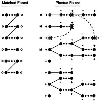
In order to facilitate augmentation on more than a couple of alternating trees, we keep a root field for each blossom, which identifies the root of the alternating tree the blossom is on. Since at the beginning each tree consists of a single blossom, initially rootj = j,W j € Gs· Whenever we grow a pair of matched blossoms to a tree, we make root fields of this pair equal to their parent’s root field. In this way one can find the root of any blossom on an alternating tree in 0(1) time. When an augmenting path between a pair of alternating trees is found, in order to differentiate them from the rest of PF, we mark the roots of the trees involved, by changing the signs of their root fields to negative. We will call such trees as marked trees. The pair of blossoms
causing the augmentation is put into the pair list PL so that the augmenting paths may be traced back towards the roots later on at the end of the stage. In Figure 3.1 dotted edges are the matching edges, whereas the dashed ones are augmenting. The roots of trees on which augmenting paths are already found are marked, denoted with the letter M in the same figure. Inscribed in squares are those blossom pairs that are listed in PL.
Matched Forest Planted Forest
- + · + M + · ----· ·-#
X\
- + V M -I-·----»»»«g) \
Figure 3.1: Marking trees, where augmenting paths are found
Marked trees are not carried to M E immediately. When a tree is marked, current minimum reduced costs of the edges between blossoms on the marked tree and 0 labelled blossoms of unmarked trees in P F are inserted to FibA, Thus for the rest of the nodes in P F , nodes in marked trees behave as if they are in MF] conversely, since at the beginning of the stage reduced cost of the edges between 0 labelled blossoms and those © labelled blossoms on marked trees were put in FibA, for the nodes in M F blossoms in marked trees behave as they are in PF. We may still grow marked trees until the end of stage. However cis for the other blossoms on marked trees, reduced cost of the cut edges from those grown pairs to 0 labelled blossoms of unmarked trees are kept in FibA as well. Note also that we will not perform any dual variable or reduced cost update for the cut edges of those pairs at the end of a stage. The
CHAPTER 3. MULTIPLE AUGMENTATION ALGORITHM 30
T he M ultiple A ugm entation Algorithm : while PF 7^ 0 do begin 5 ^ 0 ; Scan(A:),VA: € PF; while (1) do begin <- FindminO; if (6 = €a) if rooti > 0 Grow(i, j); else break; if (6 = €b) begin
if {i and j belong to the same tree) Shrink(t, j); else M ark(t,y); end if (€ = (c) Expand(t); end Update(fc); € PF : rootk > 0 Full_Update(); Multiple_augment(PZ/); end Recover( MF);
stage will continue until there is a grow from a marked tree to an unmarked tree in P F ; that is until the first time two augmenting paths intersect. We detect this case easily, since the root of a pair to be grown from a marked tree has a negative value in its root field.
Our Scan operation differs from that of Ball L· Derigs in allowing to scan the edges between marked trees and © labelled blossoms on unmarked trees. When a 0 labelled blossom i is grown to a blossom j on a marked tree with its mate, heap entry for i is deleted from Fib A. However, we do need the reduced costs of edges between marked trees and unmarked trees in P F be kept in
FibA. For this reason it is necessary that we scan i to put the relevant edge
with minimum reduced cost to FibA. Note that the same blossom will not be scanned again during a stage.
In the Mark operation we only mark the trees where the augmenting path is found. Those trees are not moved to MF. The pair of blossoms causing
Scan(i) begin
if (/6,· = ©) then
for V(ib,i) G A (i): b{k) = i do begin
if (/i»6(i) = 0) or (roo<(,(j) marked) then
FibA^f^j) m\n{FibAbQ),Ckj + wjt + Wj + «};
if (Jbh^j) = ©) and (b(j) i) and {rootf,(j) unmarked) then
FibBk(j) ^ min{Ft65fc(j), 0.5(citj - (e - d{,(_,·)) + + tn_,) + c};
if ( Ckj + Wk < Vj - (f - ¿6(p>)) + «^p>) then
Vj <- Ckj·,
Vi k;
end else
if (/6, = 0 ) and (rooti unmarked) then
FibCi Vi + €]
if (rooti marked) then
for V(A:,y) G A (i): b(k) = i do begin
if (Ihu) = ©) and (rooti,^j^ unmarked) th en
FibAi m\n{FibAi,Ckj - (e - ¿6(i)) + + wj + e};
if (ckj + Wj < V k - ( e - d^p^^) + n(pfc)) th en
Vk *- Ckj; Pk
end
end /* Scan */
the augmentation is put into the pair list PL. We said that when a tree is marked, current minimum reduced costs of the edges between blossoms on the marked tree and 0 labelled blossoms of unmarked trees in P F are inserted to
FibA. Reason for this is detecting an intersection of augmenting paths. This
is the case when minimum comes from an edge between a marked tree and a
0 labelled blossom on an unmarked tree. In order to do that without scanning
the blossoms on marked trees, we extend Lawler’s idea for keeping reduced costs of edges between 0 labelled blossoms and 0 / 0 labelled blossoms in an array, say v. In our algorithm, we additionally keep the minimum reduced cost of edges between two 0 labelled blossoms in v array. Hence, we use the at hand information in v array, which is obtained through scanning of new
0 labelled blossoms in P F and avoid rescanning blossoms in marked trees
CHAPTER 3. MULTIPLE AUGMENTATION ALGORITHM 32
paths. This is the case when minimum comes from an edge between a marked tree and a © labelled blossom on an unmarked tree. At any time during a stage, if Cij is the reduced cost of edge ( i,j) between two © labelled blossoms
6®,· and b^j at the beginning of the stage, updated reduced cost c,j is equal
to Ci j — (c — — ( c — d b ^ j ) + Wi + W j . Hence, for q G Real(k®) and a ©
labelled blossom 6(p,)®, c,p, is u, - (e - djt®) - (e - <Î6(p,)®) + u>, + where
( q , P q ) is the edge with minimum reduced cost value from g to a © labelled
blossom because v, «issumes the value of c,p, at the beginning of the stage. With a similar argument, updated reduced cost of an edge ( q , P q ) , between a
0 labelled blossom and a ® labelled blossom 6(p,)® equals to u, + (c — dfce) — (e — dj,(p^)®) + Wq + Wp^. Below, T,· denotes the alternating tree rooted at blossom i. Even though updating dual variables of blossoms on marked trees and the reduced cost of their cut edges may be delayed to the end of the stage, we find it convenient to update them while marking.
M ark(i, j) begin s ··— root,·; t <— rootj; roots *----s; roott <---- 1‘, P L ^ P L + [ijy, for VA: G T, U Tt do begin if (Ibk = ®) then
FibAk <- min{t;, - (e - djt) - (f - db(pq)) + Wq + Wp^ + e : q e Real(k)};
else
if (/6jt = 0 ) then
FibAk <- min{v, + (f - dk) - {( - d6(p,)) + «’? + «^p, + f : 9 € Real(k)};
end
Update(fc) VA: G T« U Tt; end /* Mark */
At the end of a stage, dual variables of blossoms on unmarked trees and the reduced costs of their cut edges are updated. Note that for edges between marked and unmarked trees reduced costs are partially updated in Mark. Now that all the augmenting paths found throughout the stage are stored via the pair list PL, augmentation on the marked trees can be done. Multiple.augment
operation swaps the matched and unmatched edges on augmenting paths and moves all of the marked trees to M E at once. Obviously, efficiency of the algorithm increases as the number of trees marked per stage gets larger. M ultiple_augment( PL)
begin
A ugm ent(iJ) , V [t,j] € PL] end /* Multiple-augment */
The complexity of the algorithm is O(n^) when implemented as described above. There are at most n/2 stages (n/2 is achieved if only a single augmenting path is found in every stage). At each stage an edge is scanned only either when blossom of one of its end nodes is labelled 0 or when grown to a marked tree with 0 label. Since such blossoms remain in P F until the end of stage, scanning of an edge occurs at most two times in a stage. Dual variable updates and all other operations including marking are done at most in 0 { n ) time. Observe that reduced cost updates of edges are performed at the end of a stage, except for in Mark. Partial update on reduced costs for edges that have one end in marked trees are performed while marking, but there is no second update for those at the end of the stage. Hence overall reduced cost update in a stage takes 0 ( m ) . Since any of the 0 { n ) operations can be called at most 0 { n ) times, each stage takes 0{n^). For 0(nrn log n) complexity we utilize splittable heaps.
Although, update after expand can be done in 0(log n), this time scanning of each edge takes O(\ogn) time rather than 0(1). With a little more care in the implementation of the blossoms a stage can be done in 0 (m logn). Hence, we achieve an 0 (nm log n) complexity for the algorithm.
Chapter 4
SINGLE STAGE
ALGORITHM
Here we present a single stage primal-dual algorithm [2] for the minimum cost perfect matching problem. That is, contrary to other approaches we do not stop a stage to initialize shortest paths until the algorithm finds the optimal solution. By initialization of shortest paths we mean to scan all of the blossoms in P F and building up the three Fibonacci Heaps that will be used throughout a stage. Dual feasibility is achieved by re-scanning some nodes, only when the need arises. Information on the need for rescanning is kept in one addi tional array. As a result, time consuming shortest path initializations at the beginning of each stage is totally eliminated. Elimination of initialization pro cess at an expense of re-scanning some blossoms throughout the algorithm has experimentally proved to be very effective.
The single stage algorithms performs all operations in one stage. Here, we totally eliminate the initialization of shortest paths, that is scanning of blossoms in P F at the beginning of stages. Instead, we only scan necessary blossoms in Pivot operation. In the following we will describe the reasons for re-scanning when initialization of shortest paths is eliminated, and show the possibility of maintaining dual feasibility without initialization. Then we will