Seasonality in inflation volatility: evidence from Turkey

(1)

EVIDENCE FROM TURKEY

M. Hakan Berument* Bilkent University

Afsin Sahin Gazi University

Submitted May 2008; accepted July 2009

This paper assesses the presence of seasonal volatility in price indexes where a similar type of pattern has been reported in asset prices in financial markets. The empirical evidence from Turkey for the monthly period from 1987:01 to 2007:05 suggests the presence of seasonality in the conditional variance of inflation. Thus, inferences for the models that do not account for the seasonality in the conditional variance will be misleading.

JEL classification codes: E31; E37, E30.

Key words: inflation volatility, seasonality, EGARCH.

I. Introduction

Economists are interested not only in the level of inflation but in its volatility because the latter also adversely affects economic performance.1_{The purpose of}

* M. Hakan Berument (corresponding author): Department of Economics, Bilkent University, 06800 Ankara, Turkey; phone: +90 312 2902342, fax: +90 312 2665140, e-mail: berument@bilkent.edu.tr, URL: http://www.bilkent.edu.tr/~berument. Afsin Sahin: School of Banking and Insurance, Gazi University, 06500 Ankara, Turkey; phone: +90 312 582 1100; fax +90 312 221 3202; email: afsinsahin@gmail.com. URL: http://afsinsahin.googlepages.com. We would like to thank two anonymous referees and Rana Nelson for their helpful comments.

1_{Hafer (1986) and Holland (1986) report the negative effects of inflation volatility on employment.}

Friedman (1977), Froyen and Waud (1987) and Holland (1988) argue that there is a negative relationship between output and inflation volatility. Wilson (2006) suggests that increased inflation volatility is associated with higher average inflation and lower average growth. Berument and Guner (1997), Berument (1999) and Berument and Malatyali (2001) find a positive relationship between inflation volatility and interest rates.

(2)

this paper is to assess whether there is any regularity in inflation volatility. To be specific, we will assess whether there is any seasonal pattern in the conditional inflation variability series by considering seasonally unadjusted as well as seasonally adjusted monthly data.2_{Understanding any seasonal pattern in inflation volatility}

is important. First, more efficient estimates of inflation forecasts will be gathered by better modeling conditional inflation variances. Second, if seasonal patterns exist using seasonally adjusted data, one may need to develop a new set of algorithms that addresses the seasonality in volatility. Third, since inflation volatility explains the behaviors of other macroeconomic variables, addressing the seasonality of inflation volatility may help to better capture the effects of inflation volatility on those variables.

There are a limited number of studies that analyze the determinants of inflation volatility. Bowdler and Malik (2005) provide evidence that openness reduces inflation volatility. Smith (1999) and Engel and Rogers (2001) argue that exchange rate volatility explains part of price volatility, and Ghosh et al. (1996) claim that pegged exchange rates are associated with significantly lower variability. Similarly, Bleaney and Fielding (2002) find that countries that peg exchange rates have lower inflation volatilities than floating-rate countries. According to Rother (2004), activist fiscal policies may have an important impact on inflation volatility, and volatility in discretionary fiscal policies increases inflation volatility. Aisen and Veiga (2008) argue that higher degrees of political instability, ideological polarization and political fragmentation are associated with higher inflation volatility. Dittmar et al. (1999), Gavin (2003) and Berument and Yuksel (2007) discuss the effect of inflation targeting regimes; Grier and Perry (1998), Kontonikas (2004), and Berument and Dincer (2005) point out the effect of inflation on inflation volatility. All these studies analyze the effect of economic and political variables on inflation volatility. The aim of this paper is to model inflation volatility by considering seasonal patterns of the general Consumer Price Index (CPI) inflation and its sub-components.

This paper provides evidence regarding the seasonal pattern of Turkish inflation volatilities for the period from January 1987 to May 2007. Although most prices are set monthly in Turkey, price changes make their biggest adjustment once a year –at the beginning of the year or when a new set of products enters the market. For some products, prices are generally set to include the expected inflation for the year,

2_{Similar analyses have been performed on stock market volatilities since the mid-1980s. See, for}

(3)

The credibility of the government’s policies is assessed with the announced targets when the budget details are released at the beginning of the fiscal year. Thus, one may expect that volatility reaches its peak at the beginning of the fiscal year – January. Thus, it is expected that for most products and for the general CPI, January has the highest volatility. For some other products, prices are quite seasonal, such as those for food, or prices are set mostly by the rest of the world, such as those for automobiles.4_{However, for agriculture, new seasonal products enter the market}

around April and May, and for automobiles, around July and August. Thus, one may expect that food and transportation volatilities peak around April-May and July-August, respectively. In regulated sectors such as health and housing, volatility is at its minimum just after a month after the price increases made because most adjustments for the year are made in the previous month or towards the end of the fiscal year when firms are close to finalizing their balance sheets.

The paper is organized as follows: Section II introduces and elaborates on the data. Section III introduces the model employed in the paper. Section IV reports the empirical evidence, while Section V provides a set of extensions of our models as robustness tests. The last section concludes the paper.

II. Data Characteristics

We gathered data from the Turkish Statistical Institute (TurkStat) covering monthly periods from January 1987 to May 2007. We examine the Consumer Price Index and its seven components to determine if there is any seasonality in the conditional variances for these series. The indexes that we consider are: Consumer Price Index (CPI), Group Index of Clothing (Clothing), Group Index of Culture, Training and Entertainment (Culture), Group Index of Food-Stuffs (Food), Group Index of Home Appliances and Furniture (Furniture), Group Index of Medical Health and Personal Care (Health), Group Index of Housing (Housing) and Group Index of Transportation and Communication (Transportation). Figure 1 reports the graphs of the variables.

3_{Government plays a big role in Turkey both in its share in the economy and its regulatory power. For}

example, Nevzat Saygilioglu (a former acting Treasury under-minister) argued that the share of the government sector to total income reached was around 70% at a particular point in the sample we consider (see Aydogdu and Yonezer 2007, pp. 387-397).

4_{The Turkish domestic automobile industry is integrated with the rest of the world. Moreover, a sizeable}

portion of automobile sales are of imports; the share of imports to consumption is 66% for 2007 (see Automobile Manufacturers Associations 2008).

(4)

Table 1 reports various diagnostic tests. Panels A, B and C report the unit root tests of the price indexes that we consider in their logarithmic form, with a constant (Panel A), with a constant and time trend (Panel B) and a constant in logarithmic first differences (Panel C). Each panel reports unit root tests for seasonally unadjusted

Figure 1. Graphs of observed data series (logarithmic, monthly change, seasonally unadjusted)

CPI Clothing

Culture Food

Furniture Health

(5)

Table 1. Preliminar y diagnostic tests CPI

Clothing Culture Food Fur niture Health Housing Trans. P anel A.

Unit root with log le

vels and constant

A1. Seasonally unadjusted DF -0.7960 -0.7888 -0.9133 -0.2043 0.7974 -0.4415 -1.4335 0.4881 ADF -1.9599 -1.7796 -2.0432 -2.2506 -2.4737 -1.6244 -1.9028 -2.4117 PP -1.8273 -1.7532 -1.7574 -2.5022 -1.4249 -1.9505 -1.4825 -1.4913 KPSS 2.016 *** 2.004 *** 2.011 *** 2.013 *** 2.009 *** 2.012 *** 2.022 *** 2.016 *** A2. Seasonally adjusted DF -0.6992 0.3205 0.8137 -0.1216 0.8022 0.2545 -0.5638 0.152 ADF -2.234 -1.8055 -2.0758 -2.4231 -2.4667 -2.4782 -2.3538 -2.5477 PP -2.0375 -2.2798 -1.5993 -1.621 -1.5772 -1.614 -1.7808 -1.5318 KPSS 2.016 *** 2.004 *** 2.011 *** 2.013 *** 2.009 *** 2.012 *** 2.022 *** 2.016 *** P anel B

. Unit root tests with log le

vels,

constant and trend

B1. Seasonally unadjusted DF -1.4488 -1.9233 -1.2233 -0.8415 -0.1233 -1.0753 -2.3477 0.8917 ADF 3.0511 -0.8529 0.3526 2.1247 2.8131 3.6435 -0.9223 1.7452 PP 2.7186 1.2749 2.536 2.0695 2.4438 2.9563 2.8143 2.5841 KPSS 0.443 *** 0.442 *** 0.447 *** 0.455 *** 0.434 *** 0.440 *** 0.4191 *** 0.4367 *** B2. Seasonally adjusted DF -0.2038 -0.9135 0.5845 0.1308 -0.1896 -0.1257 -0.9313 0.9809 ADF 3.1345 0.4079 2.5193 2.3901 2.4884 1.8037 0.5312 1.8603 PP 2.9457 3.0107 3.3137 3.2791 2.3762 2.335 2.6934 2.5523 KPSS 0.4433 *** 0.4418 *** 0.4473 *** 0.4558 *** 0.4350 *** 0.4406 *** 0.4191 *** 0.4368 ***

(6)

Table 1 (continued). Preliminar y diagnostic tests CPI Clothing Culture Food Fur niture Health Housing Trans. P anel C.

Unit root tests with log differences and constant

C1. Seasonally unadjusted DF -3.1422 *** -2.7039 *** -4.5638 *** -3.7773 *** -2.8519 *** -2.7378 *** -1.8769 * -4.1816 *** ADF -3.1331 ** -4.111 *** -5.5032 *** -4.8523 *** -5.6521 *** -3.8260 *** -2.7954 * -5.4529 *** PP -8.381 *** -8.701 *** -11.652 *** -9.493 *** -9.476 *** -11.973 *** -8.526 *** -11.100 *** KPSS 1.3695 *** 1.1209 *** 1.5075 *** 1.7136 *** 1.2741 *** 1.6158 *** 1.0727 *** 1.6618 *** C2. Seasonally adjusted DF -2.4206 ** -3.1260 *** -3.5682 *** -2.4546 ** -2.0755 ** -2.0739 ** -1.9179 * -10.7547 *** ADF -3.3251 ** -2.8687 * -4.6410 *** -3.4931 *** -3.1997 ** -3.5581 *** -2.7570 * -10.7900 *** PP -6.1691 *** -5.4852 *** -12.898 *** -8.7284 *** -7.2088 *** -11.504 *** -5.6379 *** -10.790 *** KPSS 1.3695 *** 1.2637 *** 1.3381 *** 1.4085 *** 1.2798 *** 1.4221 *** 1.0855 *** 1.6737 *** P anel D

. Ljung-Box Q test statistics

D1. Seasonally unadjusted 6 [0.0000] [0.0000] [0.0000] [0.0000] [0.0000] [0.0000] [0.0000] [0.0000] 12 [0.0000] [0.0000] [0.0000] [0.0000] [0.0000] [0.0000] [0.0000] [0.0000] 24 [0.0000] [0.0000] [0.0000] [0.0000] [0.0000] [0.0000] [0.0000] [0.0000] 36 [0.0000] [0.0000] [0.0000] [0.0000] [0.0000] [0.0000] [0.0000] [0.0000] D2. Seasonally adjusted 6 [0.1871] [0.0008] [0.7272] [0.6469] [0.0054] [0.1486] [0.0199] [0.9364] 12 [0.4099] [0.0054] [0.3810] [0.6112] [0.0644] [0.1840] [0.1486] [0.9898] 24 [0.1564] [0.1715] [0.5888] [0.4286] [0.5570] [0.2818] [0.7194] [0.8834] 36 [0.5941] [0.1098] [0.0374] [0.3233] [0.6900] [0.0734] [0.6611] [0.2596]

(7)

Table 1 (continued). Preliminar y diagnostic tests CPI Clothing Culture Food Fur niture Health Housing Trans. P anel E.

ARCH-LM test statistics

E1. Seasonally unadjusted 6 [0.0000] [0.0000] [0.0000] [0.0000] [0.0000] [0.0000] [0.0000] [0.0000] 12 [0.0000] [0.0000] [0.0000] [0.0000] [0.0000] [0.0000] [0.0000] [0.0000] 24 [0.0000] [0.0000] [0.0000] [0.0000] [0.0000] [0.0000] [0.0000] [0.0000] 36 [0.0000] [0.0000] [0.0000] [0.0000] [0.0000] [0.0000] [0.0000] [0.0000] E2. Seasonally adjusted 6 [0.0131] [0.0259] [0.3529] [0.1294] [0.0135] [0.4036] [0.0442] [0.8251] 12 [0.0222] [0.1252] [0.0002] [0.0123] [0.0381] [0.2154] [0.0893] [0.9869] 24 [0.2066] [0.3822] [0.0012] [0.0369] [0.4489] [0.1123] [0.5556] [0.8413] 36 [0.1958] [0.7668] [0.0018] [0.1924] [0.6662] [0.0365] [0.9767] [0.2826] Note: p-v

alues are repor

ted in brack ets. *** , ** and

*indicate rejection of the null at the 0.01%,

0.05% and 0.10% le

vels,

respectiv

ely

(8)

and adjusted series.5_{We consider four unit root tests: Dickey-Fuller (DF), Augmented}

Dickey-Fuller (ADF), Phillips-Perron (PP) and Kwiatkowski, Phillips, Schmidt and Shin (KPSS). For DF, ADF and PP, the null hypothesis is unit root (rejecting the null suggests stationarity) and for KPSS, the null is stationarity (rejecting the null suggest non-stationarity). Panels A, B and C overall suggest that the series that we consider have a unit root in log levels, but the differenced series do not have a unit root. Thus, we carried our analyses for the indexes in their logarithmic first differences. Panel D of Table 1 reports the p-values of Ljung-Box Q test statistics for 6, 12, 24 and 36 lags of the series in their logarithmic first differences. Panel E of Table 1 reports the ARCH-LM tests of the same series for 6, 12, 24 and 36 lags. We reject the null of no autocorrelation for the non-seasonally adjusted data, but no general pattern appears for the presence of autocorrelation for the seasonally adjusted data. However, the strong contrast between Panels D1 (for the seasonally unadjusted series) and D2 (for the seasonally adjusted series) suggests a strong presence of seasonality in the mean equation of the seasonally unadjusted series.

Panel E of Table 1 reports the ARCH-LM test statistics.6_{The null hypothesis}

that there is no ARCH effect up to order q in the residuals fails to be rejected when we employ seasonally unadjusted data for all the lag orders that we consider. When we employ seasonally adjusted data, the null is rejected at the 5% for at least one lag order that we consider but Transportation; for Transportation we cannot reject the null for any of the lag orders that we consider. Thus, inflation volatility needs to be modeled somehow.

Table 2 reports the descriptive statistics for the general CPI and its seven components. Panel A reports the statistics when we used the original (seasonally unadjusted) inflation data; Panel B uses the seasonally adjusted data. The means of Housing, Health, Transportation and Food are higher than the CPI for both the seasonally unadjusted and adjusted data and the means of Culture, Clothing and Furniture are less than the CPI. Table 3 reports the p-values for the test statistics: the mean and variance of each item are equal to the mean and variance of the general

5_{Although the price series that we consider have a high degree of seasonality, there is no official}

seasonally adjusted data for Turkey. However, the Central Bank of the Republic of Turkey uses the Census X11 (historical, additive) procedure to seasonally adjust series in its annual reports. Thus, we used the same procedure to seasonally adjust our series.

6_{We specify the autoregressive equation with its q-lags (where q-lags are determined by the final}

prediction error (FPE) criteria, whose properties we discuss later in the text) and a constant term. When we used seasonally unadjusted data, 11 seasonal dummies are also included.

(9)

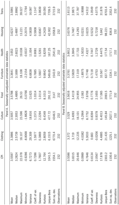
Table 2. Descriptive statistics CPI Clothing Culture Food Fur niture Health Housing Trans. P anel A.

Seasonally unadjusted univ

ariate data statistics

Mean 3.5597 3.3886 3.5057 3.5788 3.3641 3.653 3.6237 3.5981 Median 3.2824 2.5739 2.3053 3.4895 3.1699 2.6023 3.4897 2.8982 Maximum 22.078 18.107 23.596 26.53 18.108 19.038 13.221 39.027 Minimum -0.9286 -8.8068 -1.8828 -5.0766 -2.2154 -0.9337 0.2074 -1.7764 Variance 6.7273 29.309 18.816 13.625 6.6838 11.004 4.5839 16.087 Coeff. of v ar . 0.7286 1.5977 1.2373 1.0314 0.7685 0.9081 0.5908 1.1147 Sk e wness 1.7607 0.3869 2.2294 1.0114 1.5607 1.5261 0.8367 3.9839 Kur tosis 12.764 2.8059 8.4349 8.1013 9.8642 5.8259 4.2429 30.093 Jarque-Bera 1041.5 6.1515 477.72 291.12 549.65 167.25 42.002 7709.5 Sum sq. de v. 1554.1 6770.4 4346.5 3147 1543.9 2541.8 1058.9 3715.9 Obser vations 232 232 232 232 232 232 232 232 P anel B

. Seasonally adjusted univ

ariate data statistics

Mean 3.5586 3.372 3.529 3.5616 3.3761 3.6612 3.6376 3.6113 Median 3.8315 3.719 3.4093 3.4119 3.5829 3.3845 3.7467 2.9871 Maximum 20.646 12.235 16.101 24.955 17.319 17.733 14.293 37.787 Minimum 0.0989 -4.0382 -5.2964 -2.063 -1.8975 -1.5033 0.0231 -1.9088 Variance 4.7646 5.3033 8.7752 7.6706 5.7748 7.4327 3.6225 14.512 Coeff. of v ar . 0.6134 0.683 0.8394 0.7776 0.7118 0.7447 0.5232 1.0549 Sk e wness 2.0567 -0.0206 0.9378 2.1655 1.4753 1.2729 0.7218 4.0775 Kur tosis 17.878 4.4885 6.4013 17.065 10.567 6.4475 5.842 31.876 Jarque-Bera 2303.2 21.435 145.84 2093.5 637.72 177.54 98.221 8703.4 Sum sq. de v. 1100.6 1225.1 2027.1 1771.9 1334.1 1717.1 836.8 3352.4 Obser vations 232 232 232 232 232 232 232 232 Note: Coefficient of v ariation is defined as (std. de v/mean).

(10)

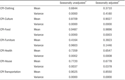
CPI for both the seasonally unadjusted and adjusted series. For both the seasonally unadjusted and adjusted series, we cannot reject the null that the mean of each of the seven sub-components is individually identical to the general CPI at the conventional 5% level.7_{When the variances of each series are examined, the variances}

of the seasonally unadjusted series are not equal to the variance of the CPI, except for Furniture. This makes sense because each series may have a different seasonal pattern. However, we can still reject the null that the variances of each of the seven items are equal to the variance of the CPI for Culture, Food, Health, Housing and Transportation at the conventional 5% level when we use the seasonally adjusted data (these results are parallel to Berument 2003 and Akdi, Berument and Cilasun 2006).

Table 4 reports the mean and variances of the CPI and its seven components for each month. The last column reports the p-values for the tests of equality for the ANOVA (Analysis of Variance) tests for means and Bartlett tests for the variances for each item across 12 months. We reject the equality of means and variances for the seasonally unadjusted data. When the series are seasonally adjusted, we cannot reject that the means of each series are equal but fail to reject that the variances are

7_{The level of significance is at the 5% level, unless otherwise mentioned.}

Table 3. p-values of the test of equality between each CPI component and the general CPI

Seasonally unadjusted* _{Seasonally adjusted}*

CPI-Clothing Mean 0.6644 0.3710 Variance 0.0000 0.4160 CPI-Culture Mean 0.8709 0.9027 Variance 0.0000 0.0000 CPI-Food Mean 0.9487 0.9896 Variance 0.0000 0.0003 CPI-Furniture Mean 0.4164 0.3923 Variance 0.9603 0.1446 CPI-Health Mean 0.7359 0.6547 Variance 0.0002 0.0008 CPI-House Mean 0.7720 0.6778 Variance 0.0037 0.0378 CPI-Transportation Mean 0.9025 0.8550 Variance 0.0000 0.0000

(11)

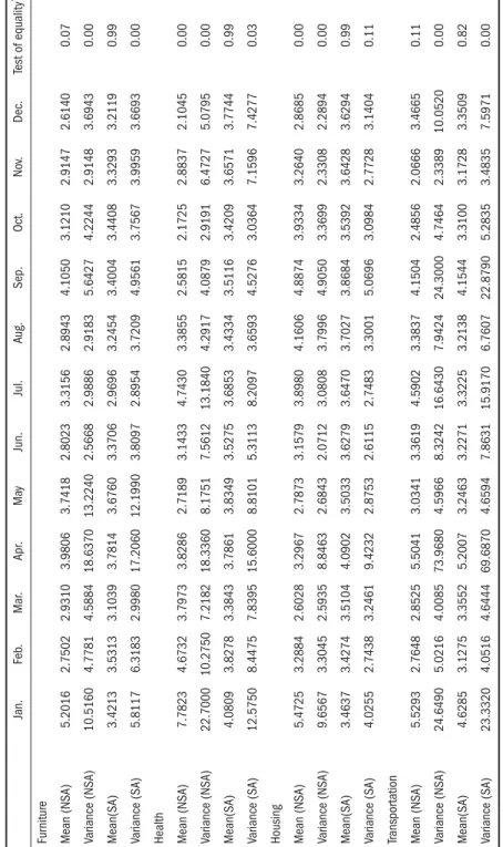
Table 4. T

est of equality across each month of the year for diff

erent price index

es Jan. Feb . Mar . Apr . Ma y Jun. Jul. Au g . Sep. Oct. No v. Dec. Test of equality

CPI Mean (NSA)

4.2000 3.2718 3.4411 5.3458 2.9996 1.3776 1.8027 2.6384 5.1182 5.4975 4.2490 2.7234 0.00 Variance (NSA) 6.0187 3.7586 3.3244 21.7590 4.2906 1.0333 2.6496 2.5773 5.5451 6.0239 3.3190 2.8045 0.00 Mean(SA) 3.6360 3.4172 3.3360 4.2752 3.4695 3.3741 3.5295 3.4661 3.6351 3.4709 3.4843 3.5949 0.99 Variance (SA) 4.3582 3.0260 2.9340 19.5450 5.1658 2.3414 3.9187 2.9842 3.9786 3.7029 3.0673 3.6883 0.00

Clothing Mean (NSA)

-2.1504 -2.5737 1.2848 10.3690 7.1558 2.6838 -1.3701 -1.2254 6.1456 11.8430 6.6061 1.7536 0.00 Variance (NSA) 7.4792 5.9868 6.1892 9.0587 5.7122 0.9580 7.5411 5.0136 7.4604 14.6030 10.5580 3.2586 0.00 Mean(SA) 2.9827 3.3691 3.4002 3.5356 3.7706 3.1365 3.4578 2.9126 3.7007 3.6264 3.4353 3.1057 0.99 Variance (SA) 5.4200 3.9198 4.3858 11.6040 5.2767 2.8206 4.8468 5.1789 6.0144 6.1208 6.3948 3.7629 0.29

Culture Mean (NSA)

Food Mean (NSA)

4.9032 5.3741 4.9416 5.6553 1.7061 -1.1489 0.3015 1.9773 4.7980 5.9943 5.2477 3.0178 0.00 Variance (NSA) 6.7521 8.3881 6.9163 35.9600 7.9784 2.2885 6.0814 6.0152 6.0866 9.3748 4.8431 6.0608 0.00 Mean(SA) 3.6379 3.3147 3.1368 4.4236 3.3536 3.4692 3.8705 3.3902 3.4984 3.5715 3.4422 3.6317 0.99 Variance (SA) 6.2288 4.2521 5.7037 30.6480 8.6871 3.4417 7.8488 6.5661 4.2922 5.8642 4.4939 6.3656 0.00

(12)

Table 4 (continued). T

est of equality across each month of the year for diff

erent price index

es Jan. Feb . Mar . Apr . Ma y Jun. Jul. Au g . Sep. Oct. No v. Dec. Test of equality * Fur niture Mean (NSA) 5.2016 2.7502 2.9310 3.9806 3.7418 2.8023 3.3156 2.8943 4.1050 3.1210 2.9147 2.6140 0.07 Variance (NSA) 10.5160 4.7781 4.5884 18.6370 13.2240 2.5668 2.9886 2.9183 5.6427 4.2244 2.9148 3.6943 0.00 Mean(SA) 3.4213 3.5313 3.1039 3.7814 3.6760 3.3706 2.9696 3.2454 3.4004 3.4408 3.3293 3.2119 0.99 Variance (SA) 5.8117 6.3183 2.9980 17.2060 12.1990 3.8097 2.8954 3.7209 4.9561 3.7567 3.9959 3.6693 0.00

Health Mean (NSA)

Housing Mean (NSA)

5.4725 3.2884 2.6028 3.2967 2.7873 3.1579 3.8980 4.1606 4.8874 3.9334 3.2640 2.8685 0.00 Variance (NSA) 9.6567 3.3045 2.5935 8.8463 2.6843 2.0712 3.0808 3.7996 4.9050 3.3699 2.3308 2.2894 0.00 Mean(SA) 3.4637 3.4274 3.5104 4.0902 3.5033 3.6279 3.6470 3.7027 3.8684 3.5392 3.6428 3.6294 0.99 Variance (SA) 4.0255 2.7438 3.2461 9.4232 2.8753 2.6115 2.7483 3.3001 5.0696 3.0984 2.7728 3.1404 0.11 Transpor tation Mean (NSA) 5.5293 2.7648 2.8525 5.5041 3.0341 3.3619 4.5902 3.3837 4.1504 2.4856 2.0666 3.4665 0.11 Variance (NSA) 24.6490 5.0216 4.0085 73.9680 4.5966 8.3242 16.6430 7.9424 24.3000 4.7464 2.3389 10.0520 0.00 Mean(SA) 4.6285 3.1275 3.3552 5.2007 3.2463 3.2271 3.3225 3.2138 4.1544 3.3100 3.1728 3.3509 0.82 Variance (SA) 23.3320 4.0516 4.6444 69.6870 4.6594 7.8631 15.9170 6.7607 22.8790 5.2835 3.4835 7.5971 0.00 Notes:

*test of equality repor

ts the p-v

alues of

ANO

V

A and Bar

tlett tests for the mean and v

ariances of series,

respectiv

ely

(13)

that even if we account for seasonality, the volatility of each series from the general CPI and the volatility of each series from each other are different. When we consider the seasonally unadjusted and seasonally adjusted series, Table 4 also suggests that the lowest variances are observed in June for the general CPI, Culture, Food and Housing; in October for Health; in November for Transportation; in June and December for Clothing. On the other hand, the highest variances are observed in April for the general CPI; October, November and April for Clothing; August and September for Culture; April for Food; April and May for Furniture; January and April for Health; January, April and September for Housing; January and April for Transportation. These highest and lowest volatilities do not take into account the dynamics of the economy and assume that positive and negative inflation shocks affect volatility in the same way. In the next section, we will employ Nelson’s (1991) Exponential Generalized ARCH model to assess any regularity in the conditional variances of inflation series.

III. Method

The economic literature suggests various methods for measuring inflation volatility, either through direct measures of volatility, by using survey data, or through indirect measures of volatility, usually by using sophisticated econometric techniques. Bomberger (1996) argues that using dispersion of the survey data measures disagreement rather than inflation volatility. Moreover, he argues that some forecasters may not want to deviate from other forecasters’ estimates, so the value of expected inflation may be biased.

The Kalman filtering and ARCH types of conditional variance modeling are the two most common sophisticated econometric techniques researchers employ to measure inflation volatility indirectly. The Kalman filter is a discrete, recursive linear filter that measures instability of the structural variability of the parameters of an equation. ARCH-type models assume that the parameters of the model are stable but estimate the variance of the residual term for the inflation specification. Evans (1991) and Berument et al. (2005) argue that the ARCH class of models is a better way of measuring risk/uncertainty, whereas the Kalman filter is better for capturing model (or parameter) instability. Therefore, we model volatility employing ARCH/GARCH models.

The conventional ARCH models are not capable of capturing the asymmetric effects of negative or positive inflation surprises on the volatility specification

(14)

(Black 1976, Engle and Ng 1993). In order to account for this, we use the EGARCH specification. The contribution of this paper is to assess whether there is any regularity in the volatility of price indexes that is beyond the dynamics of the volatility captured by the lagged conditional variance and the innovation of inflation.

Following Berument (1999 and 2003), we model inflation using lagged inflation and monthly seasonal dummies to account for seasonality. Whether seasonality is significantly related to volatility can be tested by examining the statistical significance of the estimates of each month’s coefficients. The model allows for both autoregressive and moving average components in the heteroskedastic variance.

Equations (1) and (2) give the mean and variance specifications, respectively. The mean equation is specified as:

(1) where πtis the inflation rate. Mitis for the monthly dummies accounting for monthly seasonality, wherein i = 1, 2, 3, 4, 5, 7, 8, 9, 10, 11, 12. D94tis the dummy variable that takes the value of 1 for the fourth month of 1994 to account for the 1994 financial crisis, and takes the value of zero otherwise. εtis the error term at time t. To avoid the dummy variable trap, M6t(which represents the dummy variable for June) is

not included in the specification of the conditional mean inflation. Following Hansen and Juselius (1995), we also include 13 lag values of inflation and later in the study we also consider alternative lag structures. Following Nelson (1991), we also assume that εthas General Error Distribution with mean zero and variance (ht2). Lastly, following Bollerslev and Woolridge (1992), we use the Quasi-Maximum Likelihood method to estimate the parameters.

The EGARCH representation of the conditional variance of inflation at time t is given by equation (2) as:8

(2) Here, |εt-1/ht-1| represents the absolute value of the lagged residual over the conditional standard deviation at time t – 1, (εt-1/ht-1) represents the lagged residual over the conditional standard deviation and log(h2

t-1) represents the logarithm of the conditional variance at time t – 1.

loght i it i i i it t M M 2 0 1 5 7 12 1 1

( )

= + ∑ +∑ + = = − β ψ ψ β ε / hht₋1+β ε2

(

t₋1/ht₋1

)

+β3log

( )

ht2−1. πt π θi it θ λ α i i i it t i i M M D = + ∑ + ∑ + + ∑ = = = 0 1 5 7 12 1 13 94 ππt i− +εt,

8_{See Berument et al. (2002) for the advantages of the EGARCH presentation of the conditional variance}

(15)

that inflation volatility is not explosive. If β2> 0, then a positive shock to inflation

increases volatility more than a negative shock. If β2< 0, a positive shock generates

less volatility than a negative shock. IV. Empirical Evidence

Table 5 reports the estimates of Equations (1) and (2) for the general CPI and its seven sub-components by using seasonally unadjusted data. Panel A reports the estimates of the inflation equation (Equation 1) and Panel B reports the estimates of the conditional variance equation (Equation 2). Panel C reports two diagnostic test (Ljung-Box-Q and ARCH-LM) statistics for the standardized residuals by using various lag orders and Panel D is for summary statistics. Variables M1tto M12tare

estimated coefficients for the monthly dummies.

Panel A of Table 5 suggests that the lowest monthly effects in the mean equation are observed in June for the general CPI; in February for Clothing; in November for Culture; in June for Food; in February for Furniture; in May for Health; in March for Housing; and in November for Transportation. The highest monthly effects in the mean equation are observed in October for the general CPI; in October for Clothing; in August for Culture; in January for Food, Furniture and Health; in September for Housing; in January for Transportation. These findings are parallel with the results listed in Table 4. Here, we do not interpret the estimated coefficients for the lag values of inflation but the characteristic roots of the polynomials are all inside the unit circle; thus the series are considered as stationary.

Panel B of Table 5 suggests that for the general CPI the highest volatility is in January; in September for Clothing; in August for Culture; in April for Food; in January for Furniture, Health and Housing; in July for Transportation. The lowest volatilities are observed in November for the general CPI; in June for Clothing; in December for Culture; in November for Food and Furniture; in February for Health and Housing; in November for Transportation. These findings are parallel to the expectations stated in the introduction. For the general CPI and most other items January is the month that conditional inflation variance is highest except for food (April) and Transportation (July). The lowest volatilities are observed towards the end of year except for Health (February) and Housing (February).

Next, we test whether the conditional variance is the same across each month. In particular, we test the null hypothesis that the estimated coefficients for the eleven monthly dummy coefficients are jointly zero for the conditional variance specification

(16)

Table 5. EGARCH-model parameter estimates CPI Clothing Culture Food Fur niture Health Housing Trans. P anel A. Mean specification π0 -1.8480 *** 1.1198 -0.1603 -3.7106 *** -0.0714 -0.2263 0.1728 0.1431 (0.2740) (0.6969) (0.6068) (0.8015) (0.2133) (0.2301) (0.2019) (0.4137) M1 t 2.5360 *** -3.6302 *** 2.8742 * 6.3956 *** 2.3512 *** 3.3365 *** 0.7487 * 0.8415 (0.4017) (0.7748) (1.4708) (1.9973) (0.3708) (0.5678) (0.4368) (0.5360) M2 t 1.6091 *** -4.2974 *** 0.2482 5.9633 *** -1.2511 *** 1.1145 *** -0.7050 *** -0.1017 (0.3445) (1.1319) (1.0883) (1.0823) (0.3380) (0.3409) (0.2061) (0.4514) M3 t 2.0258 *** -4.2679 *** 0.5367 4.6322 *** -0.5530 ** 1.1683 *** -0.7518 *** -0.2371 (0.3502) (1.3732) (0.7925) (1.0424) (0.2512) (0.3540) (0.2362) (0.4188) M4 t 2.3698 *** 2.2070 * -0.5097 4.6045 *** 0.8680 *** 0.1029 -0.6580 *** 0.6094 (0.4229) (1.3314) (0.8204) (1.1517) (0.2874) (0.2706) (0.2428) (0.4532) M5 t 0.9907 *** 1.2588 -0.0653 2.0689 ** -0.1734 -0.1284 -0.4040 ** -0.4323 (0.3242) (0.8885) (0.6032) (0.8496) (0.2383) (0.2690) (0.1971) (0.4483) M7 t 1.3031 *** -2.9944 *** 0.2672 2.2332 ** -0.8132 ** 1.9074 *** 0.2042 0.8013 (0.3498) (0.7634) (0.7943) (1.0369) (0.3238) (0.4077) (0.2602) (0.6617) M8 t 1.9770 *** -3.3913 *** 7.0900 *** 3.2479 *** 0.2628 1.3472 *** 0.7906 *** -0.2939 (0.3317) (1.1267) (1.7507) (1.1867) (0.2406) (0.2995) (0.2684) (0.4487) M9 t 3.4623 *** -1.1828 * 5.1377 4.6330 *** 0.7377 *** 0.0572 0.9447 *** -0.3137 (0.3704) (1.4662) (3.6908) (0.9548) (0.1924) (0.2642) (0.2872) (0.5061) M10 t 3.1521 *** 2.3453 * -0.6672 5.5139 *** 0.1475 0.3153 0.2791 -0.0833 (0.3444) (1.2714) (1.8285) (1.0446) (0.2180) (0.2816) (0.2589) (0.4895)

(17)

Table 5 (continued). EGARCH-model parameter estimates CPI Clothing Culture Food Fur niture Health Housing Trans. M11 t 2.0317 *** 0.3335 -0.9046 5.2943 *** -0.4453 * 0.2762 -0.2052 -0.7526 * (0.2993) (0.9054) (0.9818) (0.9921) (0.2455) (0.2736) (0.2392) (0.4316) M12 t 1.5123 *** -0.0571 0.4364 3.9950 *** -0.8099 *** 0.0355 -0.5819 ** -0.0724 (0.2957) (0.3796) (0.8110) (1.1566) (0.2499) (0.2405) (0.2436) (0.4393) πt-1 0.4413 *** 0.2735 *** 0.2700 ** 0.3734 *** 0.3073 *** 0.1612 *** 0.2897 *** 0.2377 *** (0.0334) (0.0525) (0.1116) (0.0767) (0.0509) (0.0310) (0.0290) (0.0334) πt-2 0.0674 -0.0952 * 0.1120 0.0848 0.3287 *** 0.1037 *** 0.0597 -0.0028 (0.0460) (0.0539) (0.0727) (0.0771) (0.0411) (0.0281) (0.0375) (0.0244) πt-3 -0.0694 0.0411 0.0652 -0.1133 -0.0208 0.0667 *** 0.1260 *** -0.0496 ** (0.0486) (0.0477) (0.0445) (0.0862) (0.0389) (0.0240) (0.0378) (0.0214) πt-4 -0.0039 0.0515 -0.0437 -0.0335 0.1484 *** 0.1087 *** 0.1042 *** 0.0699 *** (0.0337) (0.0566) (0.0500) (0.0719) (0.0339) (0.0197) (0.0347) (0.0196) πt-5 0.1340 *** 0.1083 * 0.0574 0.1978 ** 0.0233 0.0044 0.1025 ** 0.0800 *** (0.0356) (0.0609) (0.0674) (0.0834) (0.0310) (0.0259) (0.0418) (0.0238) πt-6 0.0966 *** 0.1363 ** 0.0484 0.1103 0.1476 *** -0.0043 0.1764 *** 0.0468 ** (0.0326) (0.0641) (0.0552) (0.0713) (0.0361) (0.0276) (0.0435) (0.0235) πt-7 0.0501 ** -0.0565 -0.0318 0.0220 0.0205 0.0150 -0.0661 0.0257 ** (0.0232) (0.0512) (0.0537) (0.0760) (0.0285) (0.0261) (0.0434) (0.0120) πt-8 0.0311 -0.0292 0.0682 0.0981 -0.0346 0.0220 0.0380 0.1549 *** (0.0266) (0.0472) (0.0496) (0.0696) (0.0327) (0.0173) (0.0371) (0.0175) πt-9 0.1320 *** 0.1126 *** 0.0182 0.0462 0.0164 -0.0271 0.1092 *** -0.0415 * (0.0373) (0.0417) (0.0493) (0.0829) (0.0343) (0.0199) (0.0399) (0.0233)

(18)

Table 5 (continued). EGARCH-model parameter estimates CPI Clothing Culture Food Fur niture Health Housing Trans. πt-10 0.0026 -0.0358 0.0347 0.0612 0.0267 0.0081 -0.0519 0.1055 *** (0.0335) (0.0496) (0.0550) (0.0950) (0.0387) (0.0166) (0.0381) (0.0238) πt-11 0.0072 0.1283 * 0.0234 -0.0028 -0.0435 0.0629 ** -0.0496 0.0173 (0.0341) (0.0688) (0.0583) (0.0620) (0.0343) (0.0261) (0.0358) (0.0113) πt-12 0.1021 ** 0.3489 *** 0.1387 0.0928 0.0961 *** 0.1189 *** 0.0755 * 0.0705 *** (0.0440) (0.0719) (0.0880) (0.0940) (0.0271) (0.0306) (0.0422) (0.0148) πt-13 -0.0814 *** -0.0463 -0.0315 -0.0701 -0.0473 * -0.0117 -0.0265 0.0133 (0.0325) (0.0489) (0.1005) (0.0730) (0.0279) (0.0258) (0.0330) (0.0142) D94 t 16.692 *** 6.8734 8.4826 *** 20.618 9.9576 *** 16.292 *** 9.7120 *** 35.158 *** (1.0217) (18.789) (1.3732) (50.584) (0.7700) (0.6291) (1.1787) (0.5566) P anel B . V ariance specification β0 0.4279 -2.4331 *** -1.1010 ** 1.2794 -1.7256 *** 0.3262 0.3199 1.9231 ** (0.6925) (0.8197) (0.5482) (1.5542) (0.5728) (0.7095) (0.6684) (0.8813) M1 t 0.4301 3.5656 *** 2.8491 *** -0.1654 1.9622 *** 1.8915 * 1.1003 0.2303 (0.9660) (1.1241) (0.6546) (0.8010) (0.6543) (1.1415) (0.9390) (0.8888) M2 t -0.5730 1.7888 * -0.5197 0.0381 0.3854 -1.8495 * -3.3350 *** -1.0352 (1.2994) (1.0934) (0.6954) (0.7397) (0.6686) (0.9603) (0.9612) (1.0579) M3 t -0.3812 3.8128 *** 0.0538 0.1673 0.4822 -0.2641 -0.3530 -1.2247 (0.8582) (0.9540) (0.6059) (0.7779) (0.6278) (1.0965) (0.8752) (0.7945) M4 t 0.2127 3.6230 *** 1.5603 ** 0.4873 0.6079 -1.1308 -1.1473 -1.2587 (0.9533) (0.9373) (0.6566) (0.8407) (0.6165) (1.1349) (0.8957) (0.9186)

(19)

Table 5 (continued). EGARCH-model parameter estimates CPI Clothing Culture Food Fur niture Health Housing Trans. M5 t -0.8588 2.6595 ** -0.0771 -0.1253 0.2372 -0.2514 -1.9945 * -0.5721 (1.3133) (1.1228) (0.6764) (1.0791) (0.4481) (1.1984) (1.0973) (0.8935) M7 t -0.3288 4.1994 *** 0.4563 0.3575 1.1272 ** 0.0631 -1.0397 0.3855 (1.1599) (1.4894) (0.6929) (0.6991) (0.4987) (1.2908) (1.0103) (0.8255) M8 t -1.1582 2.2973 ** 3.4971 *** 0.1250 -0.4209 -1.6579 -0.3781 -1.3342 (1.0313) (1.0749) (0.6479) (0.9247) (0.6630) (1.1652) (0.8936) (0.8581) M9 t -0.1208 4.2567 *** 1.8683 ** -0.9324 -0.3662 0.0265 -0.9316 0.0175 (0.8194) (0.9932) (0.7978) (0.8975) (0.5963) (1.1833) (0.9217) (0.9281) M10 t -1.0037 3.1697 *** -0.1863 -0.6303 0.3332 -1.2219 -1.2577 -0.7256 (0.9592) (1.0205) (0.8592) (1.1469) (0.7253) (0.9643) (0.8963) (1.0031) M11 t -2.0541 ** 2.2834 ** -0.3072 -1.2129 -0.6068 0.1051 -1.6397 * -1.5972 * (0.8228) (0.9871) (0.7383) (0.8890) (0.6805) (1.0061) (0.8417) (0.9440) M12 t -0.6633 1.2874 -0.9635 -0.2644 0.2887 -0.5649 -0.6753 -1.3507 (1.5817) (1.0012) (0.6999) (1.3330) (0.7435) (1.0607) (0.9318) (0.9300) |ε t-1 / ht-1 | 0.2642 -0.2930 ** 0.9540 *** 0.2468 2.0158 *** 0.1779 0.8279 *** 0.2683 (0.2456) (0.1363) (0.2671) (0.2497) (0.2200) (0.1720) (0.2415) (0.3623) εt-1 / ht-1 -0.1068 0.1531 0.2258 -0.0264 -0.0152 0.1586 -0.0345 0.5855 ** (0.1801) (0.0983) (0.1723) (0.1386) (0.1526) (0.1453) (0.1575) (0.2297) Lo gh 2 t-2 0.3295 0.8301 *** 0.7038 *** -0.0406 0.1909 0.9505 *** 0.8230 *** 0.0335 (0.8832) (0.0841) (0.1675) (1.1004) (0.1207) (0.0397) (0.0952) (0.2511) LRT 2.5132 53.134 *** 105.44 *** 13.2950 22.805 ** 35.113 *** 28.790 *** 6.1122

(20)

Table 5 (continued). EGARCH-model parameter estimates CPI Clothing Culture Food Fur niture Health Housing Trans. P anel C. Diagnostic tests Lags Ljung-Box Q statistics 12 [0.4450] [0.6310] [0.6010] [0.3980] [0.2380] [0.2250] [0.5200] [0.1170] 24 [0.5500] [0.7000] [0.7000] [0.5380] [0.4050] [0.2750] [0.3770] [0.2480] 36 [0.5070] [0.8440] [0.7340] [0.4780] [0.6440] [0.6030] [0.3710] [0.2440] ARCH-LM tests 12 [0.5853] [0.9572] [0.7438] [0.0706] [0.4133] [0.5827] [0.2546] [0.5731] 24 [0.3334] [0.9781] [0.5162] [0.4813] [0.0612] [0.9601] [0.4039] [0.9995] 36 [0.7442] [0.7725] [0.1852] [0.6599] [0.3199] [0.9014] [0.4941] [0.7589] P anel D . Summar y statistics GED parameter 0.9731 1.9821 192.6800 2.1339 6.6078 0.7850 1.0906 0.8500 (0.1528) (0.4410) (1196.9000) (0.5047) (2.7116) (0.1104) (0.1819) (0.1049) R-squared 0.8072 0.9075 0.4943 0.7100 0.5634 0.4370 0.7267 0.4906 Adj. R-sq. 0.7625 0.8861 0.3771 0.6429 0.4623 0.3066 0.6634 0.3726 S .E. of reg ression 1.2826 1.8525 3.4276 2.2085 1.9036 2.7587 1.2557 3.2128 Sum sq. resid 291.32 607.47 2088.10 863.35 641.45 1348.10 278.95 1827.40 D W stat 1.7116 1.6929 2.3814 1.9268 1.9758 2.0451 1.8749 1.6224

Log likelihood

-304.36 -367.29 -418.63 -447.67 -346.12 -435.91 -269.53 -451.69 Notes: Standard er

rors are repor

ted in parentheses and p-v

alues are repor

ted in brack

ets.

***

indicates significance at the 1% le

vel z = 2.58.

**

indicates significance at the 5% le

vel z = 1.96.

*indicates

significance at the 10% le

(21)

Ratio (LRT) statistics report the corresponding value. We can reject the null for Clothing, Culture, Furniture, Health and Housing. In order to see whether the month the conditional variance is maximum (or minimum) and statistically significant for the other indexes (general CPI, Food and Transportation) as reported in Table 5, we include just one dummy variable for the month corresponding to the conditional variance specification. These coefficients are statistically significant individually (not reported to save space.) Thus, we can claim that the conditional variance is not the same across each month.

In volatility specifications, our estimates of the lagged value of the conditional variances are less than one for each item; this implies that inflation volatility is not explosive (Panel B). However, there is higher persistence in the volatilities for Clothing, Culture, Health and Housing than for the others. Moreover, for Clothing, Culture, Health and Transportation a positive shock to inflation increases volatility more than a negative shock – the leverage effect. For the rest of the series, in the general CPI, Food, Furniture and Housing, negative residuals tend to produce higher variances. Panel C reports the Ljung-Box Q statistics and ARCH-LM tests for the 12, 24 and 36 lags. None of the test statistics is significant at the 5% level.

It is plausible that the results we gathered might be a type of seasonal accounting and that the estimates could be sensitive to deseasonalization. Thus, we repeat the exercise with the seasonally adjusted data (these estimates are available from the authors upon request). The lowest volatilities are in November for the general CPI and in February for Housing. Moreover, the highest volatilities in January for the general CPI, in August for Culture and in January for Furniture and Health are robust. This finding is the same for the estimates from Table 5. Furthermore, even if the volatilities in June for Clothing, in December for Culture and in November for Furniture are not the lowest, as reported in Table 5, they are the second-lowest volatilities. This exercise reveals that November for Transportation is the third lowest and the same month for Food is the fourth lowest. January is the second highest for Transportation. Last, September for Clothing and January for Housing are fourth highest. Thus, one may claim that the results from Table 5 are mostly robust.9

9_{We also tried different deseasonalization methods; although the specific month for the maximums and}

(22)

V. Extensions

In this section of the paper, we will consider a set of specifications to assess the robustness of our estimates. First, it is plausible that the seasonality in volatility may exist due to other determinants of inflation (or its volatility). In order to account for this we set up two models, both of which include a set of additional variables with a lag to both mean and variance equations. The first (unrestricted) model includes monthly dummies in the variance specification and the second (restricted) model does not include monthly dummies in the variance specification. The additional variables included in these two sets of specifications are the: squared industrial production deviation (calculated by the square of deviations from the trend obtained by Hodrick’s and Prescott’s 1997 methodology), logarithmic first difference of the exchange rate basket (basket is the Turkish lira value of the US dollar + the Euro), logarithmic first difference of oil prices (Dubai spot), logarithmic first difference of the real exchange rate; interbank rate, and an election dummy (general and local).10

As in the paper, for the seasonally unadjusted series our unrestricted model includes seasonal dummies in the variance and mean equation and our restricted model excludes seasonal dummies from the variance specification, but keeps seasonal dummies in the mean equation only. For the seasonally adjusted series, we also exclude seasonal dummies from the mean equation for both specifications. Panel A of Table 6 reports the likelihood values of the estimates that use seasonally unadjusted data and Panel B reports the same value for the seasonally adjusted data. Likelihood Ratio Test (LRT) statistics clearly reject the null that the estimated coefficients for the seasonal dummies are jointly zero in the variance specification when the other explanatory variables are included.11

Second, it is plausible that the final models are mis-specified because the same lag structure for each of the mean and variance equations for different price indexes are used. Thus, we estimate a set of models such that lag selection is determined by a set of statistical criteria for the seasonally unadjusted and adjusted data. We

10_{We gathered the industrial production, exchange rate basket and interbank rate data from the Central}

Bank of the Republic of Turkey’s electronic data delivery system. The data for oil prices is gathered from the International Monetary Fund’s International Financial Statistics Database. We constructed election dummy data from the Office of the Prime Minister, the Director General of Press and Information and the Grand National Assembly of Turkey.

11_{Both the exchange rate depreciation and the real exchange rate depreciation variables are statistically}

(23)

determine the lag length of the mean equation by considering Final Prediction Error (FPE) criteria. This is important because FPE criteria determines the optimum lag such that the error terms are no longer correlated. Cosimano and Jansen (1988) argue that if the residuals were autocorrelated, ARCH-LM tests would suggest the presence of heteroskedasticity in the residual term even if the residuals were homoskedastic. We next specified the EGARCH model by choosing lag length of possible p and q values. We used the Schwarz Bayesian Information Criterion for determining the optimum lag order for the EGARCH specification for each inflation index. Within these specifications, the unrestricted model included seasonal dummies in the variances, however, the restricted model excluded the seasonal dummy variables from the variance equation. The LRT test statistics are reported in Table 7, which reveals that we reject the null that seasonality does not exist in the variance specification for all EGARCH specifications with varying lag orders but for Food and Furniture. However, for Food, when we use both non-seasonally adjusted and seasonally adjusted data, and for Furniture, when we use non-seasonally adjusted and seasonally adjusted data, we can not reject the null. Therefore, we may claim that the results obtained from the benchmark specification are robust concerning the seasonal movements in inflation volatility.

external factors

CPI Clothing Culture Food Furniture Health Housing Trans.

Panel A: Not Seasonally Adjusted Unrestricted model -282.01 -362.19 -426.42 -388.13 -298.53 -414.6 -248.48 -400.03 Restricted model -291.30 -369.15 -443.55 -431.82 -334.24 -431.3 -261.89 -424.98 LRT 18.58* 13.90 34.26*** 87.38*** 71.42*** 33.40*** 26.83*** 49.90***

Panel B: Seasonally Adjusted Unrestricted model -251.64 -301.74 -398.16 -395.69 -321.07 -378.73 -227.38 -403.30 Restricted model -262.07 -320.09 -423.94 -407.96 -327.38 -399.66 -236.87 -426.26 LRT 20.85** _36.71*** _51.56*** _24.55** _12.61 _41.86*** _18.97* _45.93***

Notes: ***indicates significance at 0.01% level. **indicates significance at 0.05% level. *indicates significance at 0.10% level.

(24)

Table 7. EGARCH specifications with var

ying lag order

s CPI Clothing Culture Food Fur niture Health Housing Trans. P anel A.

Not seasonally adjusted

Specified models p =12 p =17 p =12 p =12 p =15 p =18 p =13 p =9 EGARCH EGARCH EGARCH EGARCH EGARCH EGARCH EGARCH EGARCH (1,2) (2,2) (1,1) (1,1) (2,2) (2,1) (1,1) (1,2) Unrestricted model -298.11 -353.37 -444.42 -451.68 -317.64 -423.24 -269.53 -439.89 Restricted model -314.65 -379.13 -479.61 -459.57 -363.49 -441.38 -283.88 -465.39 LRT 33.09 *** 51.52 *** 70.38 *** 15.77 91.69 *** 36.28 *** 28.70 *** 50.98 *** P anel B . Seasonally adjusted Specified models p =9 p =7 p =10 p =9 p =15 p =12 p =17 p =9 EGARCH EGARCH EGARCH EGARCH EGARCH EGARCH EGARCH EGARCH (1,1) (2,2) (2,1) (1,1) (1,1) (1,2) (2,1) (2,1) Unrestricted model -270.60 -343.34 -430.17 -425.00 -337.80 -398.17 -228.51 -448.80 Restricted model -285.59 -359.15 -459.51 -431.00 -344.00 -418.05 -238.13 -466.84 LRT 29.97 *** 31.63 *** 58.674 *** 10.90 12.41 39.74 *** 19.22 ** 36.09 *** Notes: (a) F

inal Prediction Criteria is used for deter

mining the lag length of the mean equation.

(b) Optimum EGARCH specificat

ions are chosen according to the Ba

yesian Infor mation Criteria. (c) LRT: Log Lik elihood Ratio Test. ***

indicates significance at the 0.01% le

vel.

**

indicates significance at the 0.05% le

vel.

*indicates significance at the 0.10% le

(25)

This paper assesses whether there is any regularity in the conditional variance of inflation using Turkish data. The empirical evidence provided here suggests that there is an increase in inflation volatility during the periods when agents set prices for the next year, at the beginning of the year or when new products enter to the markets. There is, thus, a seasonal pattern in inflation volatility and this variation has implications. First, new de-seasonality methods may be needed to address seasonality in volatility. It is a common practice to estimate conditional variance models of inflation using seasonally adjusted data but not to control for seasonality in the conditional variances. If there is seasonality in the conditional variance, then this suggests that the models are mis-specificied and subsequent hypothesis tests are inaccurate. Second, a better method of forecasting inflation may be to incorporate regularity volatility in inflation, and third, one could better model other variables that are potentially affected by inflation volatility, such as inflation volatility-growth relationships and inflation volatility-interest rate relationships.

References

Aisen, Ari, and Francisco Jose Veiga (2008), Political instability and inflation volatility, Public Choice

135: 207-223.

Akdi, Yılmaz, Hakan Berument, and Seyit Cilasun (2006), The relationship between different price indices: Evidence from Turkey, Physica A 360: 483-92.

Automobile Manufacturers Association (2008), Automotive industry annual report presentation, Istanbul, Turkey.

Aydogdu, Hatice, and Nurhan Yonezer (2007), The verbal history of the crises, Ankara, Turkey, Dipnot Press (in Turkish).

Berument, Hakan (1999), Interest rates, expected inflation and inflation risk, Scottish Journal of Political

Economy 46: 207-218.

Berument, Hakan (2003), Public sector pricing behavior and inflation risk premium in Turkey, Eastern

European Economics 41: 68-78.

Berument, Hakan, and Ebru Yuksel (2007), Effects of adopting inflation targeting regimes on inflation variability, Physica A 375: 265-73.

Berument Hakan, and Kamuran Malatyali (2001), Determinants of interest rates in Turkey, Russian and

East European Finance and Trade 37: 5-16.

Berument, Hakan, Kivilcim Metin-Ozcan, and Bilin Neyapti (2002), Modeling inflation uncertainty using EGARCH: An application to Turkey, unpublished manuscript, Bilkent University. Berument, Hakan, and Nergiz Dincer (2005), Inflation and inflation uncertainty in the G-7 countries,

Physica A 348: 371-379.

Berument, Hakan, and Nuray Guner (1997), Inflation, inflation risk and interest rates: A case study for Turkey, Middle East Technical University Studies in Development 24: 319-27.

(26)

Berument, Hakan, Zubeyir Kilinc and Umit Ozlale (2005), The missing link between inflation uncertainty and interest rates, Scottish Journal of Political Economy, 52: 222-241

Black, Fisher (1976), Studies in stock price volatility changes, in Proceedings of the 1976 Meetings of

the American Statistical Association, Business and Economics Statistics Section, 177-181.

Bleaney, Michael, and David Fielding (2002), Exchange rate regimes, inflation and output volatility in developing countries, Journal of Development Economics 68: 233-245.

Bollerslev, Tim, and Jeffrey Marc Wooldridge (1992), Quasi-maximum likelihood estimation and inference in dynamic models with time-varying covariances, Econometric Reviews 11: 143-172. Bomberger, William A. (1996), Disagreement as a measure of uncertainty, Journal of Money, Credit

and Banking 28: 381-92.

Bowdler, Christopher, and Adeel Malik (2005), Openness and inflation volatility: Panel data evidence, Working Paper 2005-W14, University of Oxford Nuffield College.

Cosimano, Thomas F, and Dennis W. Jansen (1988), Estimates of the variance of U.S. inflation based upon ARCH model, Journal of Money, Credit and Banking 20: 409–421.

Dittmar, Robert, William T. Gavin, and Finn E. Kydland (1999), Price-level uncertainty and inflation targeting, Federal Reseve Bank St. Louis Review 81: 23-33.

Engle, Robert F. (1982), Autoregressive conditional heteroskedasticity with estimates of the variance of U.K. inflation, Econometrica 50: 987-1008.

Engle, Robert F., and Victor K. Ng (1993), Measuring and testing the impact of news on volatility,

Journal of Finance 48: 1749-1778.

Engel, Charles, and John H. Rogers (2001), Deviations from purchasing power parities: Causes and welfare costs, Journal of International Economics 55: 29-57.

Evans, Martin (1991), Discovering the link between inflation rates and inflation uncertainty, Journal of

Money, Credit, and Banking 23: 169–84.

French, Kenneth R, and Richard Roll (1986), Stock return variances: The arrival of information and the reaction of traders, Journal of Financial Economics 17: 5-26.

Friedman, Milton (1977), Nobel lecture: Inflation and unemployment, Journal of Political Economy

85: 451-72.

Froyen, Richard T., and Roger N. Waud (1987), An examination of aggregate price uncertainty in four countries and some implications for real output, International Economic Review 28: 353-373. Gavin, William T. (2003), Inflation targeting: Why it works and how to make it work better?, Working

Paper 2003-027B, Federal Reserve Bank of St. Louis.

Ghosh, Atish R., Anne-Marie Gulde, Jonathan D. Ostry, and Holger Wolf (1996), Does the exchange rate regime matter for inflation and growth?, Economic Issues Series No, 2, International Monetary Fund.

Grier, Kevin B., and Mark J. Perry (1998), On inflation and inflation uncertainty in the G7 countries,

Journal of International Money and Finance 17: 671-689.

Hafer, Rik W. (1986), Inflation uncertainty and a test of the Friedman hypothesis, Journal of

Macroeconomics 8: 365-72.

Hansen, Henrik, and Katarina Juselius (1995), CATS in RATS: Cointegration analysis of time series, Estima, Evanston, Illinois.

Holland, Steven A. (1986), Wage indexation and the effect of inflation uncertainty on employment: An empirical analysis, American Economic Review 76: 235-43.

Holland, Steven A. (1988), Indexation and the effect of inflation uncertainty on real GNP, Journal of

Business 61: 473-484.

Kontonikas, Alexandros (2004), Inflation and inflation uncertainty in the United Kingdom evidence from GARCH modeling, Economic Modelling 21: 525-543.

(27)

Hodrick, Robert James, and Edward C. Prescott (1997), Postwar U.S. business cycles: An empirical investigation, Journal of Money, Credit, and Banking 29: 1-16.

Rother, Philipp C. (2004), Fiscal policy and inflation volatility, Working Paper 317, European Central Bank.

Savva, Christos S., Denise R. Osborn, and Len Gill (2006), The day of the week effect in fifteen European stock markets, unpublished manuscript, University of Manchester.

Smith, Constance E. (1999), Exchange rate variation, commodity price variation and the implications for international trade, Journal of International Money and Finance 18: 471-491.

Wilson, Bradley K. (2006), The links between inflation, inflation uncertainty and output growth: New time series evidence from Japan, Journal of Macroeconomics 28: 609-620.