On the QAP polytope and a related inequality system

Шч’« Т ’М ѴТГ1^ ^ i Τ'^1 i f

W ¿ i* ‘¿ Ь«л li «WI ■· i! '«#' Ά U'" i >ä » <jr M #’ ■«» J.y ·*' Й ώ ití'ІІ'’іГ i’ f ^ J‘'^>ya>y líi ϋ ^ 'чй*' «' ttUi4.'-’>ît

»., ·*1* » ^ P y»í, Λ · y“¿^22>0‘íí· »I·: 'Гуі'". - jV-w. ğ a ¿ , ΰ ί - s ■ А ^ З /

337

-(3N THE QAP POLYTOPE AND A RELATED

INEQUALITY SYSTEM

A THESIS

SUBMITTED TO THE DEPARTMENT OF INDUSTRIAL ENGINEERING

AND THE INSTITUTE OF ENGINEERING AND SCIENCES OF BILKENT UNIVERSITY

IN PARTIAL FULFILLMENT OF THE REQUIREMENTS FOR THE DEGREE OF

MASTER OF SCIENCE

By

Be§ir U. Amcaogiii

January, 1997

Gl.V-1 4θ·2-5

-R 43

І9Э=)-I ('('rtify that І9Э=)-I hcive read this thesis and that in niy opinion it is fully adequate, in scope and in quality, as a thesis for the degree of Master of Science.

Assoc. Prof. Barbaros Q. Tansel(Principal Advisor)

I certify that I have read this thesis and that in rny opinion it is fully adeciuate. in scope and in ciuality. as a thesis for the degree of Master of Science.

■Assoc. Prof. OSman Oğuz

1 certify that I have read this thesis and that in rny opinion it is fully adeciuate in scope and in ciualitv. as a thesis for the degree of Master of Science.

\

f

/ V

\ t '

X

Assoc. i t Mustafa Akgül

Approved for the Institute of Engineering and Sciences:

Prof. Mehmet Bapay

ABSTRACT

ON THE QAP POLYTOPE AND A RELATED

INEQUALITY SYSTEM

Be§ir U. Amcaogiu

M.S. in Industrial Engineering

Supervisor: Assoc. Prof. Barbaros Q. Tansel

.January. 1997

riie Quadratic Assignment Problem is computationally one of the most «lilficult NP-Hard problems. Recently, in 1996, Oguz introduced the so calh'd ’triangle constraints’ into an extended model of the Travelling .Salesman Ihoblem (TSP) in an attempt to give a full description of the TSP polytope. In this study, vve make use of these constraints in the context of the (Quadratic Assignment Problem (Q.AP). We discuss the relationships between the polytopes defined by the formulations with and without triangle constraints and we provide necessary and sufficient conditions for these constraints to give a full description of the QAP polytope. by-product of our analysis is that the triangle constraints suffice to define the QAP poly tope for n = 4.

Kty words: The Quadratic Assignment Problem, Computational Complex­ ity. Polyhedral Theory

ÖZET

QAP POLİTOPU VE İLGİLİ BİR DOĞRUSAL

EŞİTLİKSİZLER SİSTEMİ

Beşir U. Amcaoğlıı

Endüstri Mühendisliği Bölümü Yüksek Lisans

Tez Yöneticisi: Doç. Dr. Barbaros Ç. Tansel

Ocak, 1997

Karesel Atama Problemi (QAP) NP-zor problem sınıfı içinde averaj çözülebilirliği en az ilerletilmiş olan problemdir. Kısa süre önce Oğuz (1996), 'üçgen kısıtlan' olarak adlandırdığı yeni kısıtlar önerdi ve bu kısıtların Gezgin Satıcı Problemi (TSP) politopunu tamamıyla tanımladığını ileri sürdü. Biz bu çalışmada üçgen kısıtlarını QAP için kullanıyoruz. Üçgen kısıtlarını içeren ve içermeyen iki ayrı forrnülasyonun belirlediği politoplar arasındaki ilişkileri irdeliyor ve üçgen kısıtlarının QAP politopunu tamamıyla tanımlaması için gerekli ve yeterli şartları veriyoruz. Bu çalışmanın bir yan ürünü olarak, 11 = 4 için Q.AP politopuıiLin üçgen kısıtları tarafından tamamıyla belirlendiğini ispatlıyoruz.

Anahtar sözcükler: Karesel Atama Problemi, Hesaplama Karmaşıklığı, Holihedral Teori

To everyone I love on this planet

Hane mandam tipice labirinthus denotat ille Intranti largas, redeanti sed nimis artas

ACKNOWLEDGEMENT

I am mostly grateful to Barbaros Ç. Tansel for suggesting this interesting research topic, and who has been supervising me with patience and everlasting interest and being helpful in any way during my graduate studies.

1 am also indebted to Osman Oğuz and Mustafa .-Vkgiil for showing keen interest to the subject matter and accepting to read and review this thesis. Their remarks and recommendations liave been invaluable.

I ha\e to express my gratitude to the technical and academical staff of Bilkent Cniversity. I am especially thankful to my collègues M. Hakan Demir, Bahar Yetiîj Kara and Hülya Emir as the subject m atter of this thesis partially stemed out of discussion sessions involving these persons and I. conducted by

Barbaros Ç. Tansel.

Finally I have to e.xpress my sincere gratitude to anyone who have i)een of help, which I have forgotten to mention here.

C o n ten ts

1 Introduction and Literature R eview 1

2 Problem Formulation 5

2.1 0/1 Quadratic Programming Form ulation...

2.2 0/1 Linear Form ulation... 6

2..j Triangle Constraints S 3 Polyhedral R esults 11 -'Ll Necessary and Sufficient conditions for .ÿg4P = ... 11

3.1.1 A.i minors of G ' ... 16

3.1.2 Main R e s u lt... 17

3.2 Decomposition of a Nonintegral S o lu tio n ... 18

3.2.1 Decomposition of ; r ... 19

3.2.2 Decomposition oi y ... 21

3.2.3 Decomposition of 2 ... 24

3.3 A special case : QAP of size n = 4 26

CONTENTS 4 Conclusion B IB L IO G R A P H Y VITA V I11 29 31 34

List o f F igu res

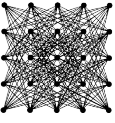
2.1 G for n = 5 ₆

2.2 The set ₈

3.1 Case n = 1 ...

C h a p ter 1

In tro d u ctio n and L iteratu re

R e v ie w

riiis study has been prompted by the work of Oğuz (1996) ou the Traveling Salesman Problem (TSP). In this study, a set of constraints called ‘triangle eonstfaints' is used to obtain tight LP based lower bounds for TSP. Oğuz ( 1996) claims that the addition of these constraints is sufficient to obtain a full description of the TSP polytope, and that the bounds are always exact. However. Oguz’s proof is still subject to scrutiny and is yet unverified as of this writing. Since The Quadratic Assignment Problem (QAP) and TSP are closely related problems (in the sen.se that TSP can be formulated as a QAP with a ■special cost structure), we decided to make use of the same concepts for Q.\P. \\'<' changed Oğuz's formulation by introducing node variables which simplified tlu' constraint structure. VVe later discovered that these constraints were also proposed by Ramachandran and Pekny (1996) as ‘three body interactions’, fhey obtain these constraints by using lifting techniciues to lift the problem to a higher dimensional space.

We do not intend to give a thorough study of the vast literature on Q.AP. Instead, we briefly describe the problem and discuss the literature most closely related to this work. The interested reader can refer to Pardalos, Rendl, and

CHAPTER 1. INTRODUCTION AND LITERATURE REVIEW

W'olkowicz (199-1) for a survey of the literature on QAP.

The Quadratic Assignment Problem is one of the most extensively studied |)rol)lems in the literature. It was first formulated by Koopmans and Beckman ( 1957) as a mathematical model for a set of indivisible economical activities.

Given a set of activities A' = {1, · · ·, n} and n potential locations for these activities, assign each activity to a location, i.e. find a permutation tt of the

set Ai, such that the total cost is minimized. The total cost consists of the cost of locating activities to given locations, and the cost of interaction between pairs of activities which is a linear function of the amount of interaction and distance between activity pairs. Formally, given A = [a,j], B = [bij], C = [c,y], an instance of Q .\P is defined by

n n Tl

X] + X] Qn-(z)

i = l j = l ¿=1

where II is the set of all permutations (i.e. assignments) of {1, ···,« } , with .1. B, C G It can be shown that the linear terms can be eliminated from the problem, hence we restrict our attention to the problem instances with no linear term. More will be mentioned about formulations of Q.AP in Chapter 2.

Despite the fact that Q.AP has extensively been studied , relatively little l)rogress has been achieved in terms of computational efficiency. The size of the largest problem solved exactly that has been reported in the literature is 50 (Resende, Rarnakrishnan, and Drezner (1995)). However, the best known exact algorithms (usually branch-and-bound type algorithms) have reportedly bo'en successful mostl}' for instances of size n < 20. For n > 20, solution times of these algorithms tend to be prohibitive except for few cases. However note that tho'se are rough measures based on the computational experience to date.

1 here remains much to be done in the computational research on QAP. rite methods of finding optimal solutions to Q.AP include dynamic programming, cutting plane, and branch-and-bound techniques. Among these, branch-and-bourid is the most successful one. An excellent survey of solution methods for Q.AP can be found in chapter 3 of Padberg and Rijal (1996). The main reason for QAP instances that lend themselves to exact solution

l)eing small is due to the difficulties in obtaining lower bounds. The ideal lower bounds should be sharp and fast to compute. For QAP, easy to compute bounds such as Gilmore-Lawler bound (Gilmore (1962), Lawler (1963)) cpiickly detoriate as QAP size grows. .Another category of lower bounds are bounds based on the Eigen values of the matrices A and B in the Koopmans-Beckman formulation (Hadley, Rendl, and Wolkowicz (1992), Rendl and Wolkowicz (1992)). These bounds are acknowledged to be the best lower bounds for Q.AP. but also the most expensive to compute. There are other bounds which are mostly based on reformulations of QAP (Assad, and Xu (1985), Carraresi. and Malucelli (1992)). Lower bounds based on Linear Programming are also reported to be good by Resende, Ramakrishnan, and Drezner (1995), Resende <'t al. (1996), and Ramachandran and Pekny (1996). LP based bounds have not drawn much attention until recently since these bounds are difficult to compute due to the sheer size of the LP relaxations of QAP. However, after ix'cent developments in interior point algorithms for linear programming, there is a growing interest on LP based lower bounds. Resende, Ramakrishnan. and Drezner (1995) point out the difficulties with commercially available LP solvers, and use an implementation of an interior point algorithm to solve large scah' LPs. The algorithm is called ■Approximate Dual Projective' (.ADP) and is (h'scribed in Karmarkar and Ramakrishnan (1991). Later. Resende et al. (1!)9()) use .\DP again to solve LP reUixations ot the higher order formulations of Ramachandran and Pekny (1996). They obtain exact bounds for Q.APs with size n < 12.

Cfi.AFTER 1. INTRODUCTION AND LITERATURE REVIEW 3

Oral and Kettani (1992) and Kettani and Oral (1993) take a different approach, and they obtain linear MIP formulations with fewer 0/1 variables, f hen they use commercially available MIP solvers to solve Q.AP instances. 1 hey report instances of size 15 in Kettani and Oral (1993), but these instances are not from the much used suite of test problems QAPLIB (Burkard, Karish. and Rendl (1991)). Padberg and Rijal (1996) point out the shortcomings of this approach.

Mathematical study of the QAP polytopes have not drawn much interest formerly, and now there is a growing interest in this direction. Padberg

CHAPTER 1. INTRODUCTION AND LITERATURE REVIEW

and Rijal (1996) give a thorough study of location, scheduling, and design [)robleius in the common framework of Boolean Quadratic Problems with Si)ecial Ordered Sets (BQPSs). QAP polytopes are studied in chapter 7 of this book. However, higher order formulations are not included (also see .lunger and Kaibel (1996) and Junger and Kaibel (1996)). .Nevertheless ])olyhedral structure of Q.AP has not been exploited yet as in the case of other combinatorial optimization problems.

C h a p ter 2

P ro b lem F orm ulation

2.1

0 / 1 Q u a d r a tic P r o g r a m m in g F o r m u la tio n

The following is a classical integer ciuadratic programming formulation of QAP.

n n n n

(QAF) m in E E E E c.j.ixijx,

i=ij=i k=i i=i / (1)

bjtct to n E = 1 i=i , i — [,■■·. n (•2) n E = 1 i=l J = 1 , · · · . /; (••I) Xij G {0. 1} A < i j < »■ ₍₁₎ The l)inar\· variables Xij represent the assignment of object i to position j ( i.e. .r/l = 1 if object i is assigned to position j . and xij — 0 otherwise), c,/^ is the cost of simultaneously assigning object i to position j , and object k to position /. If Cjj/,./ is computed using the matrices /1 and B in Kooprnans-Beckman formulation (i.e. Cijki = (likbji)·, this results in the 0/1 integer c[uadratic formulation of the Koopmans-Beckmann model. In the general case. Ciju values are arbitrarv.

CHAPTER 2. PROBLEM FORMULATION

Figure 2.1: G iov n = 5

2 .2

0 / 1 L in ea r F o r m u la tio n

To linearize the quadratic 0/1 formulation above, we first give a graph theoretic interpretation of the QAP.

bet G — (V^E) be the graph defined as follows. V = [ij : i . j = 1,· · · ,n}

E = {(ij, kl) : i J - 1, · · ·, n, i ^ k j ^ 1}

It is convenient to view G as a graph where nodes are arranged in n rows and n columns with the ith row, i?,·. consisting of nodes ¿i, i2. · · ·, in, and the jth column. Cj, consisting of the nodes 1/. 2/, ··■ ,nj. If we associate R; with object i. and Cj with position j , then the selection of node ij corresponds to assigning object i to position j . With this convention, an assignment of objects to positions induce a subset 5 of V, where S contains exactly one node in each row and each column of G. A drawing of G for n = 5, where nodes are arranged as discussed above, is given in Figure 2.1.

For ease of notation we denote edge (u, n) by uv when necessary, and define the sets :

E(r„,) = [ u v e E : u G /?,} E{C„v) = [uv e E : u e C,}

P(H,.v) is tiie set of edges whose one endpoint is v while the other endpoint lies on row i. E(c,.v) is analogous.

Note that G contains an edge between every pair of nodes, except between those that are in the same row or the same column. Therefore, the maximum clique number of G is n. and any minor of G contains exactly one node in t'ach row and each column. By a A'„ minor of G, we mean a subgraph of G which is a complete graph on n nodes. These subgraphs of G play a central role in our study. There is a natural correspondence between the n x n permutation matrices and the A'„ minors of G. If we associate costs Cijki + Ckuj with edges ( ij. kl) of G, Q.AP is equivalent to selecting a minimum arc weight A',, minor of Li. Defining the variables x,. . Ve G and y« . Ve 6 A, Q.AP can be formulated as the following linear integer program.

CHAPTER 2. PROBLEM FORMULATION 7

.<abject to m in X; Ceye teE (5) E -i·. = 1 (6) E -f. = 1 t'ec·, , i G (1. · · · ,n } ( ') E ,!/e - .i‘<; = 0 ,Ve G V. Vi G ( 1. · · •, /r} : V ^ Hi (8) E .!/e - -i‘f = 0

EEfc,.v, , VcG K Vz'G ( 1. · · ·./;.} : u ^ C\ (9)

Xv € { 0 . 1 } , V G V (10)

G { 0 . 1 } , e G A ₍₁₁₎

W’e refer to the constraint sets (6) and (7) as rowwise and columnwise assignment constraints, and to (8) and (9) as rowwise and columnwise flow constraints. The LP relaxation of (IPl) is used to obtain lower bounds for Q.AP in Resende, Ramakrishnan. and Drezner (1995). Although the relaxation gives quite good bounds, the bounds can be tightened by adding a set of constraints, riiese are the ‘triangle constraints’ mentioned in Chapter 1. This formulation is used in Resende et al. (1996) to obtain exact bounds for QAPLIB problems up to size T2. W^e define these constraints in the next section.

CHAPTER 2. PROBLEM EORMULATION

» · · · ·

• · · ·

·

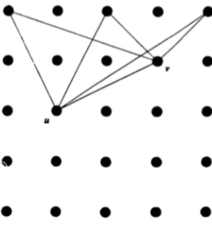
Figure 2.2: The set T{Ri,uv)

2 .3

T r ia n g le C o n str a in ts

VVe define T to be the set of node sets of A3 minors of G. An element of T is a set of three nodes in V, say {u,u,s}, such that the subgraph of G induced by is a A'3 minor of G. For ease of notation, we denote uvs = {u, u ,6’}. T is then defined as

T = {iivs : uvs is the node set of some K3 minor of G'}

We refer to the elements of T as Triangles’. .Note that uvs G T iff no two of (/., (-•..s are in the same row or the same column. Define the following sets analogous to E(c\.v) and E^fi^ ^,y.

T{R,,t) — {uvs E T : s G Ri } , Vi such that e IT A; = 0 F(c.,e) — € T : s G Ci} , Vi such that e IT G,· = 0

where t -- uv. I\R„f,) contains the node sets of A'3 minors whose one tip is in Ri and which contain the edge uv. T[c\,e) is similar. The set T(r^^uu) for n = b is shown in Figure 2.2. Define the variables Zt . Vi G T.

Rowwise and columnwise triangle constraints are defined as follows: ~t — t/e = 0 ,Ve G A , Vi such that e IT A, = 0 (12)

CH AFTER 2. PROBLEM EORMULATION

"I’lie liiglier order formulation, (IP2) below, contains all three sets of assignment, flow, and triangle constraints, as well as the 0/1 requirements on variables x, 1/. and r. (/P-2) subject to ( 5) ( 6),( 7) ( 8). (9 ) ( 12),( 13) ( 10), ( 11) G {0, 1} , i € r ( U )

Note that one can drop the 0/1 requirements on variables y, and r, and formulate the problem as a mixed integer one. This is due to the fact that 0/1 requirements on x, together with the remaining constraints, imply y^z ^ {0, 1}.

(IP2) contains node variables, " edge variables, and

triangle variables. .As a general closed formula, the number of Kp minors of G is /^(„ p)C(,i.p), where P(n.p) and C(n.p) are the p-permutations and p-combinations of n. respectively. There are 2n a.ssignment. 2rC{n — 1) flow, and /P(n — l) '( n — 2) triangle constraints.

We introduce some notation here which we use in the following chapters. .\ii ‘/i-clique’ of G means a AT minor of G. Let C = {S,A) be an /i-clique of G. where S C V, and .4 C E. The "characteristic vector’ of C — (.S', .4) is d(4ined as follows: ■Vo = 1 if u e S 0 otherwise . for V G V ’ 'i — 1 if e G v4 0 otherwise

1

\ i t c s

CHAPTER 2. PROBLEM EORMULATION 10

if (.r. //, “) is a vector of appropriate dimension satisfying eciuations (6)-(9), (I'i). (Id), the support graph of (x ,y ,z ) denoted by 6 '(x,y,;) = (H,A). is the following subgraph of G: V € H if Xv ^ 0 V ^ H if O-’u = 0 e e .4 if 2/e ^ 0 A if j/e = 0 , for V G V" , for e Ç. E

Note that the above definitions easily apply to the vectors in the (x.y) s[)ace. So the characteristic vectors of ri-cliciues are defined just the same in the {x,y) space simply by deleting the ^ part of the definition. The definition of the support graph is already independent of the variables. Observe that the support graphs of 0/1 integer solutions of (IPİ) and (IP2) are n-clic(ues of a .

It is easy to verify that (IP2) is ec[uivalent to (IP l) in the sense that the solutions of the two problems are in one-to-one correspondence, and the objective function values of the corresponding solutions are the same. .A solution of (IPl) induces a unicpie solution of (IP2) by the following construction:

Let {x,y) be a .solution of (IPl) and let G(x_y) = ( H, A) be the support graph of {x,y). The induced ~ values are

1 \ U C H

0 otherwise j e T

On the other hand, if ( x, y, z ) is a solution of (IP2), we obtain a unicpie solution of (IPl) by simply truncating the ^ part. (x, y) is a solution of (IPl) becau.se all constraints of (IPl) are contained in (IP2).

C h a p te r 3

P o ly h e d r a l R e su lts

In this chapter, vve study the relationships between the solution sets of the integer programs (IPl) and (IP2), and their LP relaxations. We use the terms ■/i-clique' and 'characteristic vector of an n-clique' interchangeably. .-Mso we sometimes use the term ‘node" instead of ’the variable corresponding to a node", ’eflge' instead of 'the variable corresponding to an edge', etc. The meanings are ( lear from the context.

We have two linear integer programs, I P \ and I P 2. Let Sip^ and .S'/P2 l>e the solution sets of I P{ and I P'2, respectively. Let Hip\ and ///P 2 be the convex hulls of these sets. Finally, let Slpi and SiP2 be the polytopes dehned l)v the LP relaxations of I P i and 7P2, respectively. Oğuz (1996) claims that [[¡P2 = Spp>. This is his main claim, and P=i\'P follows as a corollary by the polynomial definition of Slp2- However, as we pointed out. his proof of

the claim H[P2 = S i p 2 is still subject to close scrutiny. In his proof, he proposes a decomposition scheme for a nonintegral solution in Spp2 to show th at all points in Spp2 are convex combinations of n-cliques. This scheme decomposes the {x,y) part of a solution (,r,i/,-.), using r values, with respect to one column only. It is not clear how the 2: part is luindled. One can argue t hat it suffices to decompo.se the {x,y) part only. This is true in fact, but if the (x. y) part can be decomposed into n-cliques. It is clear that the decomposition with respect to one column gives solutions that have integer entries in that

CHAPTER 3. POLYHEDRAL RESULTS 12

coluniM, but not necessarily in the remaining ones. So these solutions must b(' subject to further decomposition with respect to the remaining columns until finally the {x,y) part of the original solution is decomposed into n- (ii((ues. d'his obviously neccessiates, according to Oguz’s scheme, :: values for the intermediate solutions as well as the original one. Since the c part of the origiiicd solution is not treated properly, the decomposition scheme can be api)lied only once with respect to one column, which prevents us from recursive ai)plication to reach n-cliques in the end. Nevertheless, there is a merit in the idea of projection of {x,}j,z) vectors onto the space of {x.y) vectors. VVe first discuss this idea, and later propose a decomposition scheme similar to Oguz’s but one that handles the ^ part. However, for this scheme to be applicable, (■('itivin conditions should be satisfied. We define these conditions and show that they are necessary and sufficient for ///P 2 = S'lp2· Decomposition is then

• lescribed. Discussion of the projection idea is what follows now.

We know that the projection of ff/p2 on the space of x.ij variables is ///P I. We noted that the e.xtreme points of the two .sets are in one-to-one correspondence while discussing the equivalence of (IPl) and (fP2). E.xtreme |)oints of both sets are the characteristic vectors of u-cliques of G. and the e.xtreme points of ///P 2 are projected onto the extreme points of ///p i by simply tiuncating the r part of the {x, y, z) vectors. Then, all points in the two sets can lie put into one-to-one correspondence. .-Vn interior point ( x. y. z) in ////>2 is a convex combination of some extreme points of ///P 2, and the projection of this |)oint in ///P I is the convex combination of the projections of these extreme points.

We also know that ///p i 7^ ¿Tpi. i.e. there are instances of QAP where the solution of the LP relaxation of I P l gives a nonintegral solution with objective function value strictly less than the optimal value of I Pl (see Resmide, Ramakrishnan. and Drezner (1995) ). So there are points in .S'/,pi which are not convex combinations of the 0/1 solutions of I Pl . The set of such points is .S/,pi \ IIIPl. Now, the question is whether the addition of triangle constraints cuts off all such points from Sip\. In other words, we wonder if

C'HAFTER 3. POLYHEDRAL RESULTS 13

IIii'i is the projection of S^p2 on the space of x,ij. Denote this projection by: 5* = {(:r,2/) 6 : 3{x, y, z) e 5'lp,}

In order to show P = NP, it suffices to show S ’ — ///p i by the following reasoning:

Assume S ’ = H[pi. Let { x , y , z ) ’ be an optimal solution of LP2. and let its objective function value be zpp2. zpp2 is a low^er bound for ~iP2· -¿P2 is also a lower bound for zjpi because the optimal objective function values of (IP l) and (IP‘2) are the same. It is well known that the optimal objective function \alue of the linear program solved on the conve.x hull of the integer solutions of an integer program gives the optimal objective function value for that integer program. .So, finding a point in ///p i with objective function value '-LP> is sufficient to show that Z[pi — zipi since zipi is a lower bound for zjp\. Such a point is either an e.xtrerne point of Hipi, or lies on a face of optimal solutions for the linear program on ///p i. (.r..y)‘ is just one such point in ///p i because {x~y)’ € i p p i by our assumption, and its objective function value is :/,P2 since only y variables appear in the objective function. This implies that w(' can obtciin the optimal value for I Pi by solving LP 2 whose length is a polynomial function of the input size for the Q.AP instance. T his means that t he decision version of QAP which is A’P-complete can be solved in polynomial t ime.

It is easy to show Hip\ Ç S ’:

P ro p o s itio n 1 Hipi Ç S ’

Proof: Let (.r,y) € ///p i. Then there e.xists constants cri, · · · ,a,, such that

= (.r,y) ; ¿ a . · = 1 : a, > 0.1 = 1,· · · ,c/

¿=1 ¿=1

where {(.r. .!/)^ · · ·, (.r, yY] = Sj pi.

CHAPTER :l POLYHEDRAL RESULTS U

S i r i c SLr-2- This implies E L i 2/ , - ) ‘ = (:i-,2/,~) G S'lp2 since Slp2 is a

convex set. Hence (a·, y) € 5'”. □

VVe have not been able to show S* C Hjpi, hence we don’t know whether ,S'“ = H[pi. The condition 5* = ///pi is a necessary condition for Hjpz = Slp2,

and sufficient for P = NP. Then one can concentrate on showing 5 “ C H[pi, i.e. one needs to show that if a nonintegral vector {x.y) is not a convex combination of 0/1 vectors in Sipi then there exists no c such that (.r./y. r) G Sr.p2· However, this approach may lead to a vicious cycle since it may reciuire

a characterization of convex combinations of solutions in 5’/pi, which itself is sufficient to define Hip\.

In this study, we take another direction and provide necessary and sufficient coiufitions for H[P2 = Slp2< wluch Oguz(1996) claims to be true. Throughout

the rest of the text, we denote ///P 2 by Sqap·, and Slp2 by S^p.

3 .1

N e c e s s a r y a n d S u fficien t c o n d itio n s for

S

= S

First we state a preliminary result that will facilitate our reasoning:

L e m m a 3.1 'Fake arbitrary {x, y, z) G ¿l f· intfgrr

solution, then has at least one column, say with p [p > 1) nonzero nodes, say · · · .Xup· d convex combination of n-cliques iff it is a convex combination of p points in Sip where each of these solutions contains exactly one node in column Cjq, with positions of these nodes corresponding to the positions of the nonzero nodes in the original solution. Formally, [x. y. z] is a con vex combination of n-cliques iff the following condition holds:

p

{x. y, z) = OikiTTlTc)'' k=l

CHAPTER 3. POLYHEDRAL RESULTS 15

riiis lemma is useful in that it is not necessary to explicitly gi\e a (h'composition to prove that a given a solution ( j, tj. ~) is a convex combination of /(-cliques. Rather, it suffices to show that it can be decomposed with respect to an arbitrary column satisfying the conditions of Lemma 3.1. .\fter that, Lemma 3.1 provides a recursive decomposition.

proof of L em m a 3.1 :

{only if) Suppose ( x, y, z ) is a convex combination of 0/1 vectors. {.r, y, r)''} = 5'/p2· L e t/ = {1,···,^ } . By assumption, (.c, y, z) = J2 «¿(•*'5 i/> ^ . «.· > 0 f or i e /

iei iei

Define the sets

h = {« G / : (.r,.//, z f has = 1} f or k = 1. · · ·. p .\ovv {x. y, z) can be rewritten as:

Let

{x, y, z) a ,(.r..y ,r)‘ k=i ieik

P

riiis is true since ai = 0 if z ^ (J h · Denote ^-l

(.r..y,.r)^· = ~ Y OCi{x,y,zY = Y — { x , y , z ) ‘ ■^'^k ie,tk teik

It is clear that cv; — since those and only those vectors whose indices are in If; has x^^ = 1. Also, > 0 by the nonnegativity of a,· and x^^. Then (.■/·. //. z)^ € S'ip because it is a convex combination of certain /r-cliques. and we have

{x. y, z) ^ Y Y a,{xzy,zy = Y x . J x f j f T z ) ^ k = l i q l k k = l

( if) This part is quite straightforward. Suppose the condition of the lemma holds. If has p nodes in Cj^, it can be decomposed into p solutions. <‘ach with only one node in Cj^. If these p solutions are //-cliques, then we are done; else each can further be decomposed since we assumed that the condition holds for arbitrary {xpy^z). We can continue until finally {x. y. z) can be expressed as a convex combination of n-cliques. □

CHAPTER 3. POLYHEDRAL RESULTS 16

3.1.1

K.\

m in ors o f

G

ill Older to provide necessary and sufficient conditions for Sqap = Sip , vve will make use of A’l minors of G'. Define f to be the set of node sets of K 4 minors of G. An element of U is a set of four nodes in V^, say {u, iks. r}. such that the

subgraph of G induced by {u, i.gs,r} is a K 4 minor of G. For ease of notation, we denote uvsr = { li.e .s.r} . G is then defined as

[J = {uv.sr : uvsr is the node set of some K4 minor of 6 '}

VVe refer to the elements of U as ‘quadruplets'. Note that uvsr G f iff no two of u. r,.s, /· are in the same row or the same column. Define sets:

f € U : r G Ri} , V/ such that t n /?, = 0 U(c\.t) ‘ {uvsr G U ; r G Ci] , Vi such that t D G, = 0

where t = uvs. Define the variables u-v .Vu G U. Now the two set of equations that are of critical importance are

u-’u — = 0 , y t €. T , Vi such that i fl /?, = ₍₁₎

(·->)

uGl'i c, ,t)

VV’e wilt show that Sqap = S'lp iff a certain feasibility problem related to ( 1) and (2) has a solution for certain values of c. Define

)^(

n-2)-Z = [ z £ i R « : 3 { x . y , z ) e Sr^p}

Z is the projection of S'lp onto the space of :r variables. VVe want to

know whether for arbitrary z ^ Z, system of equations (1) and (2) has a iionnegative solution in u. We cast this problem in the following form: Given ,:· = (zi,· ■ ■ .Z\r\)^ let ~ = { г ı.···,^ ı,C2. · · · , - 2,···,~ |τ|■ ···.~ |7·|}· Find a.’, if it exists, such that

( 'HA P TER 3. POLYHEDRAL RES VETS

(F P i)

Auj — z u > 0

uiicre .-lu,· = 5 is the system of equations ( 1) and (2). Note that in 5. eadi triangle variable, appears 2p times, where p = n — 3 (because p of ('((uations ( 1) and p of equations (2) have righthandsides equal to z j.

For a Q .\P of size n = 5, A can be viewed as the transpose of the node­ edge incidence matrix of an undirected graph. G = (V, E). .4 has exactly two nonzero entries equal to one in each row. The elements of V correspond to tlie quadruplets in f/, and the edges of G correspond to the equations ( 1) and (2). W ith this interpretation, (FPI) turns out to be the problem of assigning weights to the nodes of a graph in such a way that the weight of each edge is ecitial to the sum of the weights of its endpoints. Edge weights come from the solutions of (LP2) in the sense that every solution in Sl p? defines an instance of (F P I).

For a Q .\P of size n > o we can generalize the above idecis by replacing an (ndinary graph by an hypergraph. 0 — (V, S). Each hyperedge oft? corresponds to one of the equations (1) or (2) and contains exactly n — 3 nodes. This time, (F P I) is tlie problem of assigning weights to the nodes of an hypergraph in such a way that the weight of an hyperedge is equal to the sum of the weights of the nodes in it.

3 .1 .2

M ain R esu lt

.Now we are readv to state our main result.

T h e o re m 1 Sq a p — Spp iff (FPI) has a solution for all z ^ Z

proof : {onhj if) Suppose Sq a p = Spp. It is clear that if (.r,i/.z)' is the

CHAPTER 3. POLYHEDRAL RESULTS 18

for .r*’ :

1 if a G

I

1 ii G L

(x\ y, : ) ~ Y ^ «¿(.r. y, zY , У] a,· = 1 , a,· > 0 f o r i € I

tel iei

\vli(4-e {.i\ y, z f , ■ · ■, {x. y. z)'i is an enumeration of 0/1 solutions of (IP2). and / = {1. · · · , <■/}. Let now

(X = ^ a¡u,'‘ iei Obviously, uj > 0. and

Auj =

y]

iei iei iei

Hence. is a solution of (F P l) for z.

{ij) Suppose (F P l) has a solution for all z ^ Z. Pick arbitrary ( x. y. z ) Ç S'^p. and let a,· be the solution of (F'Pl) for c. If ( x. y . z ) is not an integral solution, i.e. if it has p (p > 1) nonzero nodes in a column, using a-’ it can be decomposo'd into ¡) solutions that satisfy the conditions of Lemrnad.l. Then, by Lemma 3.1,

V y .l P Sip . The details of this decomposition is given in the next section. □

3 .2

D e c o m p o s it io n o f a N o n in te g r a l S o lu tio n

In this section, we describe a method for decomposing a nonintegral solution ( x . y . z ) G Srp. provided that (FP l) is solvable for c. i.e. there exists a,’ such that ."L·' = £· .a.’ > 0. Let {x, y, z) € S f p be a nonintegral solution and sup[)ose p nodes in Cj^ have nonzero values, denoted by .гу,,. · · · .x,·,,· We need to decompose {x, y, z) into p components (j . y. c)h · · ■. (,r, /у, c)^ in order to make use of Lemma 3.1. We describe the decomposition in three separate parts corresponding to x. y. and c type variables. Whenever a component is undefined (e.g. e = (11. 13). t = (11,13,34), etc) we take its value to be zero. We denote a ciuadruplet by the union of its parts, i.e. the cjuadruplet ur.sr can l)e denoted by any one of the terms uvsr. ut, t i t 2. ихзг, where t — r.sr,

CHAPTER :}. POLYHEDRAL RESULTS 19

( 1 = uv. t 2 = -sr. fc'3 = v.'i. The same is true for triangles. But then again, the context will make the meaning clear. We also want to make an observation which we use frequently.

O b se rv a tio n 1 / / a 'node' has value zero in a solution of (LP.2), all 'edges' and 'triangles' that contain this node hare value zero in this solution, bg the constraints (S). (9). (12), (13) of (LP2). Furthermore, if (FPI) has a solution for this particular value of z. all components of ui corresponding to quadruplets

containing this node have value zero.

\o w recall that {x, g. z) is a nonintegral solution and p nodes in column i '^0 ha\'e nonzero values, (x, y, z) will be decomposed into p components corresponding to these nodes.

3.2.1

D e c o m p o s itio n o f

x

Nodes in (1 jo are decomposed into p components so that each nonzero node ill Cj,^ have value unchanged in the component corresponding to this node and have value zero in other components. Zero nodes have value zero in all components. The value of a nonzero node not in is partitioned between the components using the values of the edges between that node and the column C_{J O ·} -A zero node have value zero in all components because all the edges incident on a zero node have value zero by Observation 1.

With this scheme, for each of the p components, the sum of the node \ariables in a given column or row equals the original value of the node in

CHAPrER 3. POLYHEDRAL RESULTS 20

( ' conx'spoiicling to tliat component. Also, the sum of the values of a node in the p components ecjuals the original value of that node. These facts are very critical in restoring the conditions of Lemma 3.1, so we state them as lemmas.

Lem m a 3.2 a· = ^

C-l

proof: Take any component of x, say x^,. cci.sf ; V e Cjo :

If r = vi €. {t’l· ■ · ·, t’p} .then by construction, x[ = .t^., and .rj' - 0 for k 1.

1 hen

k=l

If r ^ {ci. · · ·, Vp} .then ,Cy = 0, and by construction x^ = 0 for k — 1. · · · ,p. Hence the lemma holds for this case

rase : r 6 V \ Cj^ : fn this ca.se,

yv,v = E y. = -i-u ^·=ı k=i reE{Cj^,v)

Tlic first equality is by construction. The second is due to the fact that the only positiv'e nodes in are Uı,···,^V< and the last equality is simply the iU)\v constraint of (LP2) relating node v and Cj^.

\'ho lemma holds for this case as well. □

Lem m a 3.3 V Pk ’ ^ ^ ’ , n veRr t'€C'. (••5) (1) for all k €. {1, · · ■ ,p}

proof: Let i € {i , - - - . n}, k € {1,···,/)}. Let Cq be the node in R, and i.e. f’o = Cj^ n Ri- Then

CIlAPTEFt 3. POLYHEDRAL RESULTS 21

11 <’o = t’t (i-i?· Ri tlie row which contains the node 1’^)

•’■'t = {xl = 0 f o r V e { H \ Vo))

vERi

If ^0 (!·<?' Hi does not contain the node vj^)

4 = Y v v , u = Y IJe = .l\; l ERi v^Ri e^Ei Pi^^vf^)

File first equality is by construction, the second is by definition of and 1 lie last equation is the flow constraint relating Ri and Vk. Hence. (3) holds for all k. .\'ow let i e {1. · · ·. n }, k e {1, · · ·, p}. ir '■ = Jo

Y 4

= E

Y 4 = Y

=

Y y. = xv.

leuce. (4) holds for all k. □

3 .2 .2

D e c o m p o sitio n o f

ij

Decomposition of ij is as follows:

i/N

0 otherwise . f o r e .'such that e n Cj^ 7^

y^ = . f o r e .•iiicli that t D Cj^ = 0

f o r k — 1. ■ · ·, p

Analogous to the decomposition of .r, the edges that are incident on one of the nonzero nodes in column Cj^ have value unchanged in the component corresponding to this node and have value zero in other components. I ’he values of edges that are not incident on column Cj^ are partitioned into components using the triangles containing that edge and a node in Cj^. Then, an edge that is incident on a row that contains a nonzero node in Cyg, sa}' c/t.

CHAPTER 3. POLYHEDRAL RESULTS ·>·>

have value zero in the component {x,y,z)^ corresponding to ct. This is clue to the fact that the node triplet containing nodes of this edge and rc· is not an eh'inent of T and its value is taken to be zero.

'The following lemmas are analogous to the Lemmas 3.2 and 3.3:

Lem m a 3.4 y = !j

k = \

proof: Consider t/« , e G i?. Caso e n Cj^ ^ 0 :

If tjf = 0. then y^ = 0 for all A: G {1, · · · ,p} by construction, hence the lemma holds trivially. If ,//e 0, then e H {I’l, ■ · ·, i»p} 0. Let v\ = e fl {c’l, · · ·, Up}. By construction, y\ — ,i/e, ancl y\ — 0 fo r \. < k ^ I < p. Hence

¿ íñ = u í ^ y e k = l

The lemma holds for this case. ( ' u s e : f n C j ^ =

In this case

.!/e = £ =t = Ve

^ J O' ’

t he first ec[Liality is by construction, the second one holds since r; = 0 for t. such that t n Cj^ / 0, but ¿D {t>i,---,Up} — 0, by Observation 1. The last ('(juality is the triangle constraint relating e and Cjg.

Hence, the lemma holds for this case as well. □

Lem m a 3.5

y

·/,

e.eE{R,,v)

= 0 , Vu G V’ , Vi G {1, · · ·, n} such that v ^ /?,· (-Ó)

XZ !Je ~ 1 ^ V'\ Vi G {1, · · ·, n} such that v ^ Cf (6) ^■€E(C„u)

CUAPTER 3. POLYHEDRAL RESULTS 23

proof: Pick V G V’, i € { I, · · · , n} such that v ^ R·,. and A· 6 { I, ■ · · , p}.

Case : V 6 {c'l, · · · ,

In tills case, v is one of the nonzero nodes in Cj^. say v = c/. If k = /, x^, = x^.. and !j^ = ,(/e /o r e ^ E such that v € e. (i.e. all arcs incident on v has value unchanged in y^. Then

and

E

E

'e = 0 f o r it ^ E such that v G t. Then

R ^ . v )

and

E i/e = 0 = -i·" The leiunia holds for this case.

( use : c Ç Cjo \ {'Oi, · · ·, Cp}

In this Ccise Xu = 0, and y^ = 0 f o r e £ E such that v € e. Then l)y construction .i/' = 0, and y^ = 0 f o r e G £’ such that c G t. for all A- G {1. · ■ ·. p}. The lerrirna holds trivially for this case.

( '<ts( : V G V \ C /

If vv(' denote e = vs using its endpoints:

E

<Â=T. >

I =

E

= E

-seR: s£Rr tez( R^.vf.v)

Siniilarlv

E

~

E

y^s ~

E

~ E

~ y^’k^ ~

•^

’i·

s€C, S€C | i€7(C,.i·^ ·.;

rii(' first three eciualities are identities, the fourth ecjuality is the triangle constraint relating R fC i ) and the edge v^v^ and the last equality is by

CHAPTER :l POLYHEDRAL RESULTS _2-i

3 .2 .3

D e c o m p o sitio n o f

So [ar, we liave not made use of values as we have mentioned. Now they will be used in the decomposition of

A _ if i^k € t

0 otherwise , fo r t .>uch that t D Cj^ ^

,Jor· t such that t D = 0 ~t —

j or k = 1, · · · . p

.\gain. analogous to the previous discussions, the triangles that are incident on one of the nonzero nodes in Cj^ have value unchanged in the component coi Iesponding to this node and hav'e value zero in other components. .A zero triangle have value zero in all components. The values of triangles that are not incident on column Cj^ are partitioned into components using the ciuadruplets containing that triangle and a node in Then, a triangle that is incident on a row that contains a nonzero node in Cj,.. say rt, have value zero in the component [ x , y , z Ÿ corresponding to Vk- This is due to the fact that the node set containing nodes of this triangle and is not an element of T and its value is taken to be zero.

I he tollowing lemmas are again analogous:

L em m a 3.6 ~ ^

k=l proof: Pick Z t - t ^ T Cast : t n Cj, ^ 0

II -Jr = 0. rf - 0 f o r k - by construction, and the lemma holds trivially. If Zt 0, then t D = r/. By construction. = zt. and

0 f o r I < k ^ I < p. Then

— ~ t

k=l riie lemma holds for this case, r «.s. .· t n = 0

CHAPTER 3. POLYHEDRAL RESULTS 25

In tills case

A:=l A*=l u^Utr

The first eciuality is by construction, the second one is true by Observation 1. 1 he last equality is one of the equalities in equations (2). The lemma holds for

this case. □

L em m a 3,7

- f — = 0 , Ve e £ ’ ,Vf such that e fl Ri

<eT(

— .i/f = 0 , Ve € £’ , Vi .stic/i that e fl C,

(7)

( S )

for all k ^ {1. · · · , p}.

proof: Let e G E. f G {1. · · · . n} such that ef] Ri = 0, and k ^ {1, · · ·, p}. C V/.sf; ; e n {t’l, · · · . Cp} 7^ 0

In this ca.se e contains one of the nodes I’l. · · ·, Cp, say vi. If k = /, then = tj,,. and = .:■( for t which contain e. Then

<iiid

If A· / /. then ,i/p = 0, ciiid ~f = 0 for t which contain e. Then

E

and

E

^^ = o = y^

The lemma holds for this case. C a s t ; t n ( C j ^ \ { u i , · · · . t’p } ) 0

CHAPTER 3. POLYHEDRAL RESULTS ¿1

made:

O b s e rv a tio n 2 If ti and ¿2 dre two distinct triangles in T, and if both are contained in u € U , then = ~t2 d solution of (LP2).

proof : P'irst note that if ¿1 and ¿2 are in the same quadruplet, they have an edge in common. Denote ¿1 by prs, and similarly, ty by rsv. where their common edge is rs. prs and rsv are contained in the quadruplet prsv. The nodes p.r.scv are all in different rows and columns. Now consider the node in the row of c, and column of p (one can as well consider the node in the column of r. a.nd row of p). Denote this node by I (see Figure 3.1). / forms a triangle with the edge rs. .A solution of (LP2) satisfies the following two constraints:

' ^ p r s “f” ' ^ I r s — ! J r s (9 )

' ^ I r s ' ^ v r s \ ) r s (1 0)

^ p r s --- ‘^ v r s · □ Ec[uations (9) and (10) imply

L e m m a 3.8 For QAP of size n = 4, (FPl) has a solution for all z ^ Z.

Proof : Proof is constructive. We will construct a solution u; for (FPl) as follows:

( 'HAPTER POLYHEDRAL RESULTS 26

/yf = 0. and rf = 0 for t which contain e. Tlie lemma holds trivially for this case.

( 'asf : e fl Cj^ —

Denote / by ev where e is an edge of t, and v is the opposite vertex of t.

E

E

E

E

w6fll “Gt ( and

E --f= E4=

E = =

The first three ecjualities are identities, the fourth equality is one of the e<|uations (1 )(equations (2)), and the last equation is by construction. Hence

the lemma holds for this case. □

.\'ow we have decomposed a given solution (.r. tj.z) into p parts. (,r, y. ~)'. · · ·. (,r. y, ~)p. f rom Lemma 3.2, Lemma .3.4, and Lemma 3.6. it follows that

k = l

.\ote that by Lemma 3.5 and Lemma 3.7. ( x. y. z)^ satisfy the flow and triangle constraints of (LP2) for k — By Lemma 3.3 (x,ij,z)^ satisfies the assignment constraints with righthandsides .zy,, instead of 1. .N'ow denote

ixTljTz)^ = — {x.y.z)^ .A· € {1,···./>} X Vk

B\· the above argument, (x, y, ~)^ satisfy all constraints of (LP2), so (.r, y, r )^' t Slp f o r k 6 {1. ···,/>}, and {x,y,z) is a convex combination of (.r, /y, z)^ by

tlu' following coefficients:

(x. y,z) = E cxkiYTyTzf k=i

where o/.· = Xv,.·

3 .3

A s p e c ia l c a s e : Q A P o f size

n = A

Lor this case we will show that Sqap = Spp. i.e. LP relaxation of (IP2) gives a full description of the QAP,\ polytope. First, there is a key observation to be

CHAPTER 3. POLYHEDRAL RESULTS 28

II. Ç. U, and assign:

U>u — ~t

when» t is an arbitrary triangle contained in u. By observation 2, u-’ is determined uniciuely, and > 0 by the nonnegativity of It is easy to see tiiat is a solution of (F P l). For n = 4. each triangle is contained in exactly one quadruplet, and the system of ecjuations of (FPl) reduce to:

uju, — Zt = 0 , Vi G T, u is the quadruplet that contains t

And these equations are satisfied by construction. □ C o ro lla ry By Theorem 1. Sqap = S i p for n — 4.

C h a p ter 4

C o n clu sio n

I he question F = N P has been in the center of computational theory for the last few decades. The question is closely related to .AI studies since most decision processes of the human mind can be modeled as combinatorial o[)timization problems which usually turn out to be A F-hard. These include theorem proving in mathematics, the most abstract creation of human mind. If it were shown that P = N P , AI would suddenly be brought into the realm of today's world (at least theoretically) and would seize to be the far dream which is the situation for .AI todav.

In these circumstances, we have been intrigued by the claim of Oğuz ( stating that the LP rela.xation of his version of (IP2) gives a full definition of the TSP polytope which immediately implies P = i\ P. The computational e.xperience of Resende et al. (1996) provided further motivation for this study. They obtained e.xact bounds from this formulation up to Q.AP size n = 12. hence there exists no counter example to Oğuz’s claim yet.

In order to show that Sqap — S'l p, one needs to show that each point in S[,p is a convex combination of some integer solutions of (IP2). This task has pro\ed to be nontrivial during our study. Although we have not been able to show Sqap = Sip which would have tremendous impact, we provided necessary

and sufficient conditions for Sqap — S i p . This clarifies the matter and gives

CHAPTER 4. CONCLUSION 30

an outline of the proof of P — N P if one wishes to use the LP relaxation of (IP3) to that effect. Of course, this is not the only way of devising a proof if it exists. Slp may not be equal to Sq a p arid still P = N P may be true.

.\nother approach is using the projective ideas discussed. One could go about proving 5* = Hipi instead of showing Sqap = S^p. The implication

in any case is P — NP . This is a reasonable approach since Sq a p = S ip is

not a necessary condition for 5'* = ///p i; in other words, S ‘ may be equal to H[pi even if Sqap ^ S^p. Hence. S" = Hip\ is a weaker condition sufficient

to imply P = NP .

.\lthough w'e have reservations about Oguz's proof of the claim Sq a p = S[,p,

the fact that the claim holds for n = 4 and the existence of no counter example for other cases yet provide some support that Oguz's claim ma\' after all be true.

We believe that our study will motivate the polyhedral approach to the solution of the Q.A.P which seems to be the most fruitful approach in the Q.A.P research. Also, the investigation of other special cases for n > 5 is facilitated l)\· our work.

B ib lio g ra p h y

[1] Assad, A.A., and VV. Xu, 1985. On Lower Bounds of Quadratic 0. I Programs. Operations Research Letters, Vol. 4, 175-ISO.

[2] Burkard, R.. .S. Karisch, and F. Rendl, 1991. Q .\PL IB -.\ Quadratic .Assignment Problem Library. European Journal of Operational Research,

Vol. 55, 11.5-119.

[•1] Cariciresi, P.. and F. Malucelli, 1992. .A .\ew Lower Bound for the Quadratic Assignmnet Problem. Operations Research Vol. 40. no. .Supplement 1. S22-S27.

[l] Gilmore, P., 1962. Optimal and Suboptimal .Algorithms for the Quadratic .Assignment Problem. ./. Siam. Vol. 10. 305--31.'3.

[5] Hadley, S.VV.. F. Rendl, and H. VVolkowicz. 1992. .A .\ew Lower Bound via Projection for the Quadratic .Assignment Problem. Mathematics of Operations Research. Vol. 17. 727-739.

[6] .Jünger, .VI., and V. Kaibel, 1996. .-A Basic Study of the Q.AP-Polytope. rechnical Report No. 96.215, Institut für Informatik, I.'niversität zu Köln. [7] .Jünger, M., and V. Kaibel, 1996. On the SQ.AP-Polytope. Technical Report

.\o. 96.241, Institut für Informatik. Universität zu Köln.

[8] Karniarkar, N.K., and K.G. Ramakrishnan, 1991. Computational Results of an Interior Point .Algorithm for Large Scale Linear Programming.

Mathemeithical Proejramming, Vol. 52, 555-586.

BIBLIOGRAPHY 32

[!)] Kettaui. 0 ., and M. Oral, 1993. Reformulating Quadratic Assignment Problems for Efficient Optimization. HE Transactions, Vol. 25, 97-107. [10] Koopmans, T.C., and M..J. Beckmann. 1957. Assignment Problems and

the Location of Economic Activities. Econornetrica, Vol.25, 53-76.

[11] Lawler. E., 1963. The Quadratic Assignment Problem. Management Science. Vol. 9, 75-94.

[12] Oğuz, 0 ., 1996. P=NP-A Full Description of the T.SP Polytope. Personal Communication.

[13] Oral, M.. and 0 . Kettani, 1992. A Linearization Procedure for Quadratic and Cubic Mixed Integer Problems. Operations Research Vol. 40, no. Supplement 1. S109-S116.

[14] Padberg. M.W, and M.P. Rijal, 1996. Location. Scheduling. Design and Integer Programming. Kluwer Academic Publishers.

[15] Pardalos. M., F. Rendi, and H. VVolkovvicz, 1994. The Quadratic Assignmnet Problem: .A Survey and Recent Developments. In .\.\IS Proceedings of the DIM.ACS workshop on QAP.

[16] Resende. M.G.C., K.G. Ramakrislman. and Z. Drezner, 1995. Computing Lower Bounds for the Quadratic .-Vssignment Problem with an Interior Point .Algorithm for Linear Programming. Operations Research, VoL 43.

781-781.

[17] Resende. M.G.C., K.G. Ramakrishnan. B. Rarnachandran, and .J.F'. Pekny, 1996. Tight QAP Bounds via Linear Programming. http://ne tlib.bell-labs.com/netlib/att/rnath/\)e.o pit/mgcr/index.html.

[18] Ramachandran. B., and .J.F. Pekny, 1996. Higher Order Lifting Techniques in the Solution of the Quadratic .Assignment Problem. In The State of the Art in Globed Optimization: Computational Methods and .Applications. pages 75-92. Kluwer .Academic Publishers.

BIBLIOGRAPHY 33

[19] Rendl, F., and H. Wolkovvicz, 1992. Applications of Parametric Program­ ming and Eigenvalue Maximization to the Quadratic Assignment Problem. Mathematical Programming, Vol. 53. 63-78.

V IT A

Be^ir U. Aincaoglu was born on March 10, 1972 in Ankara, Turkey. He received his high school education at Ankara Atatürk Anadolu Lisesi, Turkey. He graduated from the Department of Industrial Engineering, Boğaziçi University, in 1994. In October 1994, he joined to the Department of Industrial Engineering at Bilkent University as a research assistant. From that time to the present, he has worked with .Assoc. Prof. Barbaros Ç. Tansel for his graduate study at the same department.