Simulated annealing for texture segmentation with Markov models

(1)

INTERNATIONAL WORKSHOP O N INDUSTRIAL APPLICATIONS O F MACHINE INTELLIGENCE AND VISION (MIV-891, Tokyo, April 10-12,1989

SIMLlLATED ANNEALING FOR TEXTURE SEGMENTATION WITH MARKOV MODELS M. Cemal Yalabik

Bilkent University, Physics Department Ankara, Turkey

Nese Yalabik

METU Computer Engineering Department Ankara, Turkey

Abstract

In this study, segmentation of binary textured images into regions of different textures is implemented. The Binary Markov Model (BMM) is used, and model paraaeters are assumed to be unknown prior to segmentation. The parameters are estimated using a weighed least squares method while segmentation is performed iteratively using simulated annealing. To speed up the annealing process, an initial coarse segmentation algorithm which quickly determines the approximate region categories using K-means clustering algorithm is employed. The results look quite promising while the computational costs may be reduced further by optimization of the computations.

Introduction

Representation of textured images by Markov Models(MM), or Markov Random Fields (MRF) has been studied extensively in the last few years [1,2,3]

in general used to segment an image consisting of two or more different textured regions, which in practice may correspond some problems in remote sensing, biome- dical applications or robot vision such as in the ins- pection of impurities [ 4 ] .

binary, and are used for representing binary images [l], while others can be applied to gray-level images, and the models used are Gibbs Random Fields, or Gaus- sian MRFs. Various parameter estimation and segmentation algorithms such as relaxation or hierarchical segmentation are studied where model parameters may or may not be assumed to be known.

A hierarchical model where the textured region geometry may also be assumed to be a MM has been adapted in [Z],

[3]

,

and [SI. The texture parameters may be estimated by either the maximum likelihood method [l] which becomes cumbersome for high order models or a version of least squares, which gives accurate results which can be estimated efficiently for even higher order models c 2 ]

.

Model (BMM) for binary textures with the average gray level of 0.5. (The model is also of interest to statistical physicists, and we will discuss the physics perspective of our implementation in a separate section below.) The model parameters are estimated by a weighed least squares method as will be discussedbelow. The segmentation of the image into two regions of different textures is carried out in the following two steps:

a) Coarse segmentation using a fast clustering algorithm to find two modes,

b) Fine segmentation using simulated annealing. This second step iteratively moves pixels from one region to another to maximize the probability of occurrence of textures and texture geometry. This procedure involves the modeling of the image by a two level hier- archy of BMM, one level for region textures and another

.

The models are

Some of the models are

In this study, we adapt the Binary Markov

for region geometry.

The details of the segmentation algorithm and the experimental results will be discussed in the following sections.

Binary Markov Model

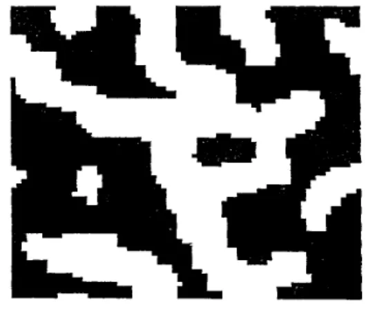
Figure 1 shows an artificially created image using two different BMM's for two different textures with another for region geometry. The generation algorithm is given in [l] and will not be repeated here.

an 8-neighborhood as in Figure 2 . In the model, the probability of finding a pixel in state x is given by

The BMM assumes

exp (xT) 1

+

exp(T)

p (X=x

I

a, b

,

c

,

d

,

e, f

,

g

,

h) =

with {x,a,b,c,d,e,f,g,h}= 0 or 1 and, T= c

where c l... c5 are the model parameters.

Here, if c = c = 0, then the model is first order, otherwise, a second order model. In this study, we performed experiments using both orders. It is also assumed in general in this study that

total number of black pixels= total number of white

+

c (a+b)

+

c3(c+d)

+

c4(e+f)

+

c5(g+h)

,

1 2

4 5

pixels for both textures.

onal constraint which results in only four independent parameters per texture.

Although this assumption may be restrictive in practice, it makes the segmentation problem more challen- ging since no average gray level information might be used to differentiate the two regions. It should be mentioned that this constraint is not essential in our implementation and can easily be relaxed whennecessary for natural textures.

This assumption brings an additi-

We assume that the two-texture image can be modeled by (and indeed, we generate our test images for the computer experiments using)

exp(yxT1

+

(l-y)xT2)

1

+

exp(yTl

+

(1-y)T2) P(X=xly,a,b,c,d,e,f ,g,h)=

where the additional binary parameter y is the (invi- sible) variable that determines the texture type at that pixel site. T and T represent terms with two different texture parameters. The variable y itself is assumed to be defined through an isotropic first order BMM in terms of its four neighbors ya, ...,y d:

1 2

(2)

Figure 1. A Mixture of two different textures

exp

I

yc (y a

+.

. .

+ Yd)

I

1

+

explc (ya +...+ y )

P(Y=ylya.

.

. .

,y,)=

d I

The joint probability is then the product of the above two expressions. The problem we have at hand, then, is the case when the x's are given, and we are required to determine a reasonable set of y's that may correspond to these pixel values.

The Statistical Physics Context

The BMM is of interest in statistical physics (SP), where it is called a "classical spin system". first order BMM is the Ising Model [ 6 ] .

Model is probably the most extensively studied model in theoretical physics, as it is the simplest system which exhibits a non-trivial order-disorder phase tran-

sition. This seemingly simple class of models have presented formidable resistance to rigorous analysis, and exact results on their properties are available only for very restricted cases. One of the more power- ful means of analysis has been the numerical simulation of the behavior of the models, which involves the generation of the pixels (corresponding quantities are called "spins" in Physics) through a Markov process (this is the "Monte Carlo" procedure in Physics [7]). Through these studies, an immense amount of knowledge has accumulated about the types of patterns that are generated by the pixels of Ising type models. On the other hand, some seemingly simple generalizations of this model present formidable problems in understanding the types of order that correspond to them. The expertise that has accumulated in the methods of analysis and their results can be a helpful guide in studies related to modeling textures as BMM. For example, it is known that models of this type become "critical" for some values of their parameters. While such critical proces-

ses are very exciting to physicists, and may be useful for modeling textures with fractal structures, it is also true that these processes have a very slow power- law approach to equilibrium in contrast to the familiar exponential approach. Hence, an attempt to generate a texture from such a process would be prohibitively slow.

The The Ising

Figure 2. A pixel X and its 8-neighbors

In this section, we at certain points refer to the ideas and results that have been in the SP literature for some time. No attempt has been made to be complete in acknowledging the vast amount of literature that exists. Instead, some typical works and a number of review ar- ticles will be cited for the interested reader.

Segmentation of a pattern into different regions corresponding to different textures involves the assignment of a new variable to every pixel whose value identifies the region.

Ising Model in Physics, within the context of renormalization group theory [8].

is not very appropriate in our context since this theory involves the identification of new larger "pixels" from a number of pixels of the textured image, resulting in a reduction of the resolution of the pattern, and hence to a renormalization of its length scale.) A crucial part of the application of this procedure involves the estimation of the parameters of the underlying Markov Process for particular sets of spin configurations (i.e. patterns) of the model. Some of these methods have been applied to the parameter estimation problem in textured images. We use one such procedure for the estimation of the parameters of the textures

1

21. Ideas that come very close to our simulated annealing procedure (which was inspired by the Monte Carlo Renormaliza- tion Group [lo] in SP) exist in the pattern recognition literature ( e . g . the relaxation algorithm discussed in

[3]) but there are important conceptual differences. One related area of study of the Ising model that does not seem to have found an application in pattern analysis is the stud

the MRF ill, 1 2 j

.

Through these methods, it should be possible to identify different regions of a time depen- dent image corresponding to textures with perhaps exactly the same MRF parameters (and hence cannot be diffe- rentiated in a static picture) but with different vari- ations in time.

The annealing step will be discussed in detail in the section on Segmentation Procedure.

will point out that if the MRF parameters for both the textures and the segmented region shapes could be estimated exactly, this procedure would result in a sequence

A similar process is carried out on the (The name "renormalization"

of the dynamics of the generation of

At this point we

(3)

of segmented patterns whose probability of occurrence would be proportional to the probability that the given textured picture was produced by those segmented patterns. This would happen after a number of steps that are required for the system to reach "equilibrium". The number of steps required for this to happen depends on the value of the MRF parameters, and may be prohibitively large for "critical" values of the parameters as was stated earlier. Our experiments with computer generated data indicate that the MRF parameters are estimated with relatively good accuracy.

If the parameters are large in magnitude (corresponding to a low "temperature" for the Ising model), fewer number of "states" will appear as a result of the above procedure (i.e. the segmentation will be more success-

ful) as these states will now have a larger difference in probability compared to the other states. In contrast, if the parameters are small in magnitude, these high temperature models will lead to higher entropies (both in information theoretic as well as thermodyna- mic sense) and the result of the segmentation is neces- sarily more uncertain.

The "annealing" procedure (as its name implies) must involve a gradual reduction in the temperature to obtain the more probable states. This is accomplished in our case automatically by the continual updating of the BMM parameter estimates. Initially, when the segmentation is not yet accurate, the estimatedparameters will be smaller in magnitude due to the reduced corre- lation resulting from erroneous segmentation. These parameters progressively grow towards their equilibrium values as segmentation becomes more accurate. We have found out that this is an important feature of the algorithm which further differentiates it from the relaxation type algorithms. In our experiments, we have found out that even if the exact MRF parameters are supplied to the annealing procedure, if these parameters correspond to sufficiently low temperatures, the system quickly relaxes to an unrepresentative state with a local probability maximum (a "quench" in SP language).

Estimation of Parameters

The BMM parameters may be estimated by using maximum likelihood estimation by dividing the image into dis- joint sets called codings. However, this approach requires the solution of nonlinear equations in general. Another approach may be described through the following equation :

In [P(x=l:a

,...,

h) / P(x=O:a

,...,

h)] = T.

This equation gives rise to a linear equation in terms of the model parameters. Here, the ratio of the proba- bilities can be estimated by counting certain combinations of a,.. .,h with x=l and forming the ratio. For- ming one equation for each combination, values of c2,.

. .

,c that will minimize the least square error can be determined. This approach was used in [2]. For the second order model there will be 81 combinations, grouping the probabilistically identical combinations

(such as a-1, b=O and a=O, b=l) together. However, certain combinations may appear very rarely for certain textures. This makes the computation more feasible. One problem with the above formulation is that the rela- tive number of occurrences of specific combinations may not reflect themselves in the result since only the ratio nl/no

result in inaccurate results. Here, n1 and no are the total number of occurrences of certain combinations with x=O and x-1, respectively. One way to avoid this

is used in the estimation and this might

problem is to weigh the effects by multiplying the individual equations by n1

+

no so that

2 error=

1

( n1

+

no) [ln(nl / no)

-

T]

,

conf ia.

_-

and using this formulation in the least squares estimation. In this study, we used this weighed least squares method. The results of the estimation will be given in the section on Experimental Results below.

Segmentation Procedure

Our segmentation algorithm is made up of two parts. In the first part, an initial estimate for the two regions is constructed through a K-means clustering approach.

A vector with a component corresponding to each term that multiplies a particular parameter of the MRF probability density function is formed for every pixel. The algorithm can then be expressed as:

1) Form the vectors

2) Average these vectors over a 2x2 window throughout the image.

3)

from the jet found in step 1 above and find the distan- ce d= I l V -V

1 1

between these vectors (city block dis- tance in our implementation).

4 ) Take another vector V, and determine the distances Choose two arbitrary vectors V1 and V2

1 2

5 ) 6) 7 )

8) Classify all pixels into two clusters based on the distances of the vectors V to V1 and V2

9)

red with respect to V1 and V2 and replace values of V1 and V with these average values.

10) Repeat steps 8 and 9 a predetermined number of times (two times in our implementation).

The success of this initial segmentation is crucial for the efficiency of the subsequent annealing procedure since this algorithm will use only the local relations- hips among the pixels. It is therefore important that the global classification of the texture is established before annealing starts. Otherwise, the annealing pro- cedure may identify a particular texture as "texture 1" and the other as "texture 2" at one part of the image, and vice versa at another part of the image. However, if the annealing time is sufficiently long, we have noticed that most images will be segmented satisfacto- rily even with a completely random initial segmentation estimate.

In the second part of the segmentation procedure, we carry out a simulated annealing procedure. This we do by first estimating the BMM parameters corresponding to the two textures (which we assume are distributed in the two regions based on the present segmentation

If dl> d then set d=di and V =V If d2> d then set d=di and V =V Repeat steps 4 to 6 for all vectors Vi.

and go to step 7. 2 i

1 i

Determine the average values of the vectors cluste-

(4)

estimate), and a global, isotropic, first order BMM parameter corresponding to the shapes of the regions. We then choose a pixel position at random and consider moving that pixel from one region to another as described below. In principle, whenever a change takes place, the parameter estimates must be renewed. Howe- ver, the parameters change very little with the change in the segmentation of a single pixel, so that the

estimation can be done once after a number of steps of the above annealing procedure. We have made no efforts towards optimizing the machine execution time for this procedure. Our program presently estimates the new texture parameters each time a segmentation change takes place, and the global BMM parameter once after an average of one segmentation change attempt per pixel. (This period of simulation is called one"Monte Carlo Step" (MCS) in SP language.) Even under these conditi- o n s , segmentation of a 100x100 image takes about 22 seconds for initial segmentation and 45 secs/MCS on a Data General MV 20000 computer.

The annealing algorithm can then be expressed as follows:

1) Based on the present segmentation estimate of the image, estimate the BMM parameters for each texture. 2) Repeat the above procedure for the estimation of the BMM parameter that controls the region geometry. 3) Choose a pixel on the image at random and consider a change in its segmentation. Suppose the segmentation variable is attempted a change from value y to 1-y. Then, compute the quantity

exp (l-y)xT1

+

yxT exp (yxT1

+

(l-y)xT2)

exp (1-2y) C(ya+ ...+y d)

.

2

P=

4) If P is greater than or equal to one, then carry out the change in the segmentation. If P is less than one, carray out the change only if P is greater than a random number R selected from a uniform distribution between zero and one.

5 ) If the segmentation change attempt is successful,

carry out the estimation process in steps 1 and 2. (In practice, this can be done somewhat less frequently: I n our implementation, we perform the estimation of the BMM parameters for the region geometry once every MCS.)

Figure a) Two regions, generated with a first order BMM

6) Repeat steps 3 to 5 a predetermined number oftimes. (Approximately 8 MCS in our implementation.)

Experimental Results

In Figure 3a, we see an image with two regions, which is generated with BMM. Figure 3b shows the same image where each region is filled with a different first order BMM texture. We observe the segmentation results in Figures 3c and 3d.

first step of our segmentation, while Figure 3d is the result of annealing. Figure 4 is another example o f our segmentation, with two second order model textures filling the regions. As it can be observed, the algorithm works successfully i n even very hard to differentiate textures as in Figure 4b.

Figure 3c is the result of the

Conclusions

It can be concluded from above results that the BMM can be used in texture segmentation of binary images successfully. Model's generality makes it applicable for many kinds of natural textures where gray level properties are not significant.

Although a cost analysis was not performed at thisstage of the study, our experiments show that with the speed- up provided by the coarse segmentation step, the method becomes quite feasible. It may also be speeded up con- siderably by future optimizations, such as those possible in the re-calculation of parameters at each iterati- on of segmentation.

The approach can be generalized to the segmentation of more than two regions in the same image, with minor modifications.

References

[l] G.R.Cross, A.K.Jain, "Markov Random Field Texture Models", IEEE Trans. PAMI, Vol.PAM1-5, No:l, Jan.1983, pp 25-39

[3] F.S.Cohen,D.B.Cooper "Simple Parallel Hierarchical and Relaxation Algorithms for Segmenting Noncausal Markov Random Fields", IEEE PAMI, Vol.PAMI-9,No:2, March 1987, pp 195-219

3

b) Regions filled with two first order BMM textures

(5)

c) Result of first step of segmentation d) Result of annealing

Figure 4

a) Two regions, generated with a second order BMM b ) Regions filled with two second order BMM textures

(6)

[4] R. W. Conners ,C. W.McMillin.K.Lin,R. E. Vasquez- Espinoza "Identifying and Locating Surface Defects in Wood: Part of an Automated Lumber Processing System", IEEE PAMI, Vol.PAM1-5, No:6, November 1983, pp 573-585

[s]

C.W.Therrien "An Estimation-theoretic Approach to Terrain Image Segmentation", Computer Graphics and Image Processing, Vo1.22, 1983, pp 313-326 [6] E.Ising, 2.Phy.s. No.31. pp 253-258, 1925 [7] K.Binder (ed) "Applications of the Monte Carlo

Method in Statistical Physics", Topics in Current Physics, Vo1.36. Springer, Berlin-Heidelberg- New York, 1984

[8] K.G.Wilson,J.Kogut "Renormalization Group and the E Expansion" Physics Report, Vol.l2C, pp 75-200 1974

[9] W. Kinzel, "New Real-Space Renormalization Techni- ques and Their Application to Methods of Various Spin and Space Dimensionalities" Vol.Bl9, No.9, pp 4584-4589, May 1979.

[LO] R. H. Swendsen, "Renormalication Group by Monte Carlo" [U] P.C.Hohenberg,B. 1.Halperin "Theory of Dynamic Cri-

Phys. Rev.Letters, Vo1.42 pp 859-861, 1979

tical Phenomena" Rev.Mod.Phys.No.49,No:2,pp 435- 520 April 1977

Methods", Phys.Rev.letters, Vo1.37, No:8 pp 461- 463 August 1976

[12] S.K.Ma "Renormalization Group by Monte Carlo