Hamiltonian equations in ℝ3

Hamiltonian equations in

R

3

Ahmet Ay, Metin Gu¨rses, and Kostyantyn Zheltukhina) Department of Mathematics, Faculty of Sciences, Bilkent University, 06800 Ankara, Turkey

共Received 8 April 2003; accepted 18 August 2003兲

The Hamiltonian formulation of N⫽3 systems is considered in general. The most

general solution of the Jacobi equation inR3 is proposed. The form of the solution is shown to be valid also in the neighborhood of some irregular points. Compatible Poisson structures and corresponding bi-Hamiltonian systems are also discussed. Hamiltonian structures, the classification of irregular points and the corresponding reduced first order differential equations of several examples are given. © 2003

American Institute of Physics. 关DOI: 10.1063/1.1619204兴

I. INTRODUCTION

The Hamiltonian formulation of a system of dynamical equations is important not only in mathematics but also in physics and other branches of natural sciences. They in general describe conserved systems. Among all possible odd dimensional cases, the three dimensional dynamical systems have a unique position. The Jacobi equation in this case reduces to a single scalar

equation for three components of the Poisson structure J. Due to this property N⫽3 dynamical

systems attracted much research to derive new Hamiltonian systems.6 –12More recently1,2a large class of solutions of the Jacobi equation inR3 was given. Poisson structures, in all dimensions, were also considered in Ref. 3. In this work, we consider a general solution of the Jacobi equation

in R3_{. We find the compatible Poisson structures and give the corresponding bi-Hamiltonian}

systems. We give all explicit examples in a special section and Table I at the end.

Let us give necessary information about the Poisson structures in R3_{. A matrix J}

⫽(Ji j), i, j⫽1,2,3, defines a Poisson structure in R

3 _{if it is skew-symmetric, Ji j⫽⫺J}

ji, and its entries satisfy the Jacobi equation

Jli⳵lJjk⫹Jl j⳵lJki⫹Jlk⳵lJi j⫽0, 共1兲

where i, j,k⫽1,2,3. Here we use the summation convention, meaning that repeated indices are

summed up. Let us introduce the following notations. For matrix J put J12⫽u, J31⫽v, J23⫽w.

Then the Jacobi equation共1兲 takes the form

u⳵1v⫺v⳵1u⫹w⳵2u⫺u⳵2w⫹v⳵3w⫺w⳵3v⫽0. 共2兲

It can also be rewritten as

u2⳵1 v u⫹w 2_⳵ 2 u w⫹v 2_⳵ 3 w v⫽0. 共3兲

关We assume that none of the functions u, v and w vanish. If any one of these functions vanishes

then Eq.共2兲 becomes trivial for the remaining two variables; see Remark 1.兴

We consider the general solution of the Jacobi equation共3兲 and show that it has the following form:

Ji j⫽␮⑀i jk⳵k⌿, 共4兲

a兲_{Electronic mail: zhelt@fen.bilkent.edu.tr}

5688

where␮and⌿ are arbitrary differentiable functions of xi, i⫽1,2,3 and⑀i jk is the Levi–Civita symbol. We also consider special solutions given by

u⳵1v⫺v⳵1u⫽0, w⳵2u⫺u⳵2w⫽0, which implies v⳵3w⫺w⳵3v⫽0. 共5兲

Such Poisson structures appear in many examples. We show that this special class of solutions belongs to the general form共4兲. We introduce these special solutions to study the irregular points of the Poisson structures. All the irregular points of the Poisson structure matrix J given in the

examples,1 we know so far, come from this special form. Hence they are also irregular points of

the form 共4兲 we give.

II. THE GENERAL SOLUTION

Assuming that u⫽0, let␳⫽ v/u and␹⫽ w/u; then Eq. 共2兲 can be written as

⳵1␳⫺⳵2␹⫹␳⳵3␹⫺␹⳵3␳⫽0. 共6兲

This equation can be put in a more suitable form by writing it as

共⳵1⫺␹⳵3兲␳⫺共⳵2⫺␳⳵3兲␹⫽0. 共7兲

Introducing differential operators D1 and D2 defined by

D1⫽⳵1⫺␹⳵3, D2⫽⳵2⫺␳⳵3, 共8兲

one can write Eq. 共7兲 as

D1␳⫺D2␹⫽0. 共9兲

Lemma 1: Let Eq. (9) be satisfied. Then there are new coordinates x¯1,x¯2,x¯3 such that

D₁⫽⳵¯_x

1 and D2⫽⳵¯x2. 共10兲

Proof: If Eq.共9兲 is satisfied, it is easy to show that the operators D1 and D2 commute, i.e.,

D1ⴰD2⫺D2ⴰD1⫽0.

Hence, by the Frobenius theorem共see Ref. 4, p. 40兲 there exist coordinates x¯1,x¯2,x¯3such that the

equalities 共10兲 hold. 䊐

The coordinates x¯1,x¯2,x¯3 are described by the following lemma.

Lemma 2: Let␨be a common invariant function of D1 and D2, i.e.,

D1␨⫽D2␨⫽0, 共11兲

then the coordinates x¯1,x¯2,x¯3 of Lemma 1 are given by

x

¯₁⫽x₁, ¯x₂⫽x₂, ¯x₃⫽␨. 共12兲

Moreover from (11) we get

␹⫽⳵1␨ ⳵3␨

, ␳⫽⳵2␨

⳵3␨

. 共13兲

Theorem 1: All Poisson structures inR3, except at some irregular points, take the form (4),

i.e., Ji j⫽␮ ⑀i jk⳵k␨. Here␮and ␨are some differentiable functions inR3

u⫽␮⳵3␨,

v⫽␮⳵2␨, 共14兲

w⫽␮⳵1␨.

Thus matrix J has the form共4兲 (⌿⫽␨). 䊐

Remark 1: So far we assumed that u⫽0. If u⫽0 then the Jacobi equation becomes quite

simpler,v⳵3w⫺w⳵3v⫽0, which has the simple solution w⫽v␰(x1,x2), where␰is an arbitrary

differentiable of x1 and x2. This class is also covered by the general solution共4兲 by letting ⌿

independent of x3.

A well known example of a dynamical system with a Poisson structure of the form共4兲 is the

Euler equations.

Example 1: Consider the Euler equations共Ref. 4, pp. 397–398兲,

x˙1⫽ I2⫺I3 I2I3 x2x3, x˙₂⫽I3⫺I1 I3I1 x₃x₁, 共15兲 x˙₃⫽I1⫺I2 I1I2 x₁x₂,

where I1,I2,I3苸R are some 共nonvanishing兲 real constants. This system admits a Hamiltonian

representation of the form共4兲. The matrix J can be defined in terms of function ⌿⫽⫺12(x1 2_⫹x 2 2 ⫹x3 2 ) and␮⫽1, so u⫽⫺x3, v⫽⫺x2, 共16兲 w⫽⫺x1, and H⫽ x₁2/2I1⫹ x2 2 /2I2⫹ x3 2 /2I3.

Recently, a large set of solutions of the Jacobi equation共3兲 satisfying 共5兲 was given in Ref. 1. For all such solutions the Darboux transformation and Casimir functionals were obtained; see Ref. 1.

Definition 1: For every domain⍀苸R3let Ia(⍀) be the set of all solutions of (5) defined in ⍀ with u(x), v(x), and w(x) being C1_(⍀).

Following Ref. 1 we have as follows.

Proposition 1: Let␩(x1,x2,x3),␺i(xi),␾i(xi), i⫽1,2,3, be arbitrary differentiable functions defined in⍀. Then the functions

u共x兲⫽␩共x1,x2,x3兲␺1共x1兲␺2共x2兲␾3共x3兲,

v共x兲⫽␩共x1,x2,x3兲␺1共x1兲␾2共x2兲␺3共x3兲, 共17兲

w共x兲⫽␩共x1,x2,x3兲␾1共x1兲␺2共x2兲␺3共x3兲,

define a solution of Eq. (5) belonging to Ia(⍀).

Definition 2: For every domain⍀苸R3, let Ib(⍀) be the set of all solutions of (5) defined in ⍀ where one of the functions u(x), v(x), and w(x) is zero and the others are not identically zero in⍀.

Following Ref. 1 we have Proposition 2.

Proposition 2: Let␩(x1,x2,x3),␰i(xi), i⫽1,2,3, be arbitrary differentiable functions defined in⍀. Then the functions

u共x兲⫽0, v共x兲⫽␩共x1,x2,x3兲␰2共x2兲, w共x兲⫽␩共x1,x2,x3兲␰1共x1兲 共18兲

define a solution of Eq. (1) belonging to Ib(⍀), u⫽0. Similar solutions can be given in the case

v⫽0 and the case w⫽0.

Remark 2: All of the Poisson structures described in Ref. 1 have the form共4兲. For the Poisson

structure J, given by 共17兲, assume ␺1, ␺2, and ␺3 to be nonvanishing and define ␮

⫽␩(x1,x2,x3)␺1(x1)␺2(x2)␺3(x3) and ⌿⫽

冕

x1␾1 ␺1 dx1⫹

冕

x₂␾ 2 ␺2 dx2⫹

冕

x₃␾ 3 ␺3 dx3;

then J has form 共4兲. For the Poisson structure J, given by 共18兲, define␮⫽␩(x1,x2,x3) and ⌿

⫽兰x_1␰

1(x1)⫹兰x3␰2(x2); then J has form 共4兲.

Let us give two examples of systems that admit a Hamiltonian representation described by the Proposition 1 and Proposition 2.

Example 2: Consider the Lotka–Voltera system,8,9

x˙1⫽⫺abcx1x3⫺bc␮0x1⫹cx1x2⫹c␯x1,

x˙2⫽⫺a2bcx2x3⫺abc␮0x2⫹x1x2, 共19兲

x˙3⫽⫺abcx2x3⫺abc␯0x3⫹bx1x3,

where a,b,c,␮0,␯0苸R are constants.

The matrix J is given by

u⫽cx1x2,

v⫽⫺bcx1x3, 共20兲

w⫽⫺x2x3,

and H⫽abx1⫹x2⫺ax3⫹␯0ln x2⫺␮0ln x3.

Example 3: Consider the Lorenz system8

x˙1⫽

1 2x2,

x˙₂⫽⫺x₁x₃, 共21兲

x˙3⫽x1x2.

The matrix J is given by

u⫽14,

v⫽0, 共22兲

and H⫽x₂2⫹x₃2. Many other examples are given in Sec. III.

In the derivation of the general solution, Theorem 1, we assumed that one of the components of matrix J is different from zero. In addition our derivation is valid only in a neighborhood of a

regular point of J 共matrix J⫽0 at this point兲. If p苸R3 is an irregular point where u( p)⫽v(p)

⫽w(p)⫽0 it is not clear whether our solution is valid in a neighborhood of such a point. Here we shall show that the Poisson structures given by共4兲 preserve their form in the neighborhood of the following irregular points.

Lemma 3: The solution of the equation (1) defined in Proposition 1 and Proposition 2 and written in the form (4) preserve their form in the neighborhood of the irregular points, lines and planes inR3 defined below

(a) Irregular points. Let p⫽(p1, p2, p3) be such that ␾1( p1)⫽␾2( p2)⫽␾3( p3)⫽0 and ␺i( pi)⫽0, i⫽1,2,3; then p is an irregular point where the general form (4) is preserved. (b) Irregular lines or irregular planes. Let p⫽(p1, p2, p3)苸R3 be such that ␩( p1,x2,x3)⫽0

关␩(x1, p2,x3)⫽0 or ␩(x1,x2, p3)⫽0] and ␺i( pi)⫽0, i⫽1,2,3; then x1⫽p1 (x2⫽p2 or

x3⫽p3) is an irregular plane, where the general form (4) is preserved. Let x1⫽p1, x2

⫽p2 be such that ␩( p1, p2,x3)⫽0 关␩( p1,x2, p3)⫽0 or ␩(x1, p2, p3)⫽0] and␺i( pi)⫽0, i⫽1,2,3 then x1⫽p1, x2⫽p2(x1⫽p1,x3⫽p3or x2⫽p2,x3⫽p3) is an irregular line, where

the general form (4) is preserved.

Proof: The solution given in Proposition 1 and Proposition 2 solves the following equations 共without any division兲:

u⳵1v⫺v⳵1u⫽0,

⫺u⳵2w⫹w⳵2u⫽0, 共23兲

v⳵3w⫺w⳵3v⫽0.

The general form 共4兲, given in Remark 2, is also preserved at such points since we can define

␮⫽␩(x1,x2,x3)␺1(x1)␺2(x2)␺3(x3) and ⌿⫽

冕

x1␾1 ␺1 dx1⫹

冕

x₂␾ 2 ␺2 dx2⫹

冕

x₃␾ 3 ␺3 dx3,

or if one of the components of J is zero, assume u⫽0, we define ␮⫽␩(x₁,x₂,x₃) and ⌿

⫽兰x_1␰

1(x1)⫹兰

x_3␰

2(x2). 䊐

Example 4: For the Euler system considered in Example 1 the Poisson structure, given by 共16兲, has irregular point p⫽(0,0,0). The irregular point p⫽(0,0,0) satisfies the conditions of

Lemma 3, the functions ⌿⫽⫺1

2(x1 2_⫹x

2 2_⫹x

3

2_{), ␮⫽1 in terms of which the Poisson structure is}

given, are well defined in a neighborhood of p⫽(0,0,0).

III. BI-HAMILTONIAN SYSTEM

In general the Darboux theorem states that共see Ref. 4兲, locally, all Poisson structures can be

reduced to the standard one 共a Poisson structure with constant entries兲. The above theorem,

Theorem 1, resembles the Darboux theorem for N⫽3. All Poisson structures, at least locally, can

be cast into the form共4兲. This result is important because the Darboux theorem is not suitable for obtaining multi-Hamiltonian systems inR3, but we will show that our theorem is effective for this

purpose. Writing the Poisson structure in the form 共4兲 allows us to construct bi-Hamiltonian

representations of a given Hamiltonian system.

Definition 3: Two Hamiltonian matrices J and J˜ are compatible, if the sum J⫹J˜ defines also a Poisson structure.

Definition 4: A Hamiltonian equation is said to be bi-Hamiltonian if it admits two Hamil-tonian representations with compatible Poisson structures,

dx

dt⫽JⵜH⫽J˜ⵜH˜ , 共24兲

where J and J˜ are compatible.

Lemma 4: Let Poisson structures J and J˜ have the form (4), so Ji j⫽␮⑀i jk⳵k⌿ and J˜i j ⫽␮˜⑀i jk⳵k⌿˜ . Then J and J˜ are compatible if and only if there exists a differentiable function ⌽(⌿,⌿˜ ) such that

␮

˜⫽␮⳵⌿

˜⌽

⳵⌿⌽, 共25兲

provided that⳵_⌿⌽⬅⳵⌽/⳵⌿ ⫽0 and⳵_⌿˜ ⌽⬅⳵⌽/⳵⌿˜ ⫽0.

This suggests that all Poisson structures inR3 have compatible pairs, because the condition 共25兲 is not so restrictive on the Poisson matrices J and J˜. Such compatible Poisson structures can be used to construct bi-Hamiltonian systems.

Lemma 5: Let J be given by (4) and H(x1,x2,x3) is any differentiable function; then the

Hamiltonian equation,

dx

dt⫽JⵜH⫽⫺␮ⵜ⌿⫻ⵜH, 共26兲

is bi-Hamiltonian with the second structure given by J˜ with entries u ˜共x兲⫽␮˜ ⳵3g„⌿共x1x2x3兲,H共x1,x2,x3兲…, v ˜共x兲⫽⫺␮˜ ⳵2g„⌿共x1x2x3兲,H共x1,x2,x3兲…, 共27兲 w ˜共x兲⫽␮˜ ⳵1g„⌿共x1x2x3兲,H共x1,x2,x3兲…, and H˜⫽h„⌿(x1x2x3),H(x1,x2,x3)…, ⌿˜ ⫽g„⌿(x1,x2,x3),H(x1,x2,x3)…, ␮˜⫽␮(⳵⌿˜⌽/⳵⌿⌽).

Provided that there exist differentiable functions⌽(⌿,⌿˜ ), h(⌿,H), and g(⌿,H) satisfying the following equation: ⳵g ⳵⌿ ⳵h ⳵H⫺ ⳵g ⳵H ⳵h ⳵⌿ ⫽ ⌽1共⌿,g兲 ⌽2共⌿,g兲 , 共28兲 where⌽₁⫽⳵_⌿⌽兩_(⌿,g),⌽₂⫽⳵_⌿˜⌽兩_(⌿,g).

Proof: By Lemma 4, J and J˜ are compatible and it can be shown by a straightforward

calculation that the equality共being a bi-Hamiltonian system兲,

J

˜_ⵜH˜_{⫽JⵜH, 共29兲}

or

␮˜ ⵜ ⌿˜ÃⵜH˜⫽␮ⵜ ⌿Ãⵜ H 共30兲

is guaranteed by共28兲. Hence the system

dx1

dx2

dt ⫽⫺␮⳵3⌿⳵1H⫹⳵1⌿⳵3H, dx3

dt ⫽␮⳵2⌿⳵1H⫺⳵1⌿⳵2H, 共31兲

is bi-Hamiltonian. 䊐

Remark 3: The Hamiltonian function H is a conserved quantity of the system. It is clear from

the expression共31兲 that the function ⌿ is another conserved quantity of the system. Hence for a

given Hamiltonian system there is a duality between H and ⌿. Such a duality arises naturally

because a simple solution of the equation 共28兲 is ⌿˜ ⫽H, H˜⫽⌿ and␮˜⫽⫺␮. Thus we have a

hierarchy of Hamiltonians that start with a Casimir of the second structure and terminates with a Casimir of the first structure. Such systems are equivalent to the quasi-bi-Hamiltonian systems of

lower dimension with nondegenerate Poisson structures共see Ref. 5, pp. 185–220兲.

Remark 4: Using Lemma 5 we can construct infinitely many compatible Hamiltonian

repre-sentations by choosing functions ⌽, g, h satisfying 共28兲. If we fix functions ⌽ and g, then Eq.

共28兲 became linear first order partial differential equations for h. For instance, taking g⫽⌿H and

␮˜⫽⫺␮, which fixes⌽, we obtain h⫽ln H. Thus we a obtain second Hamiltonian representation

with J˜ given by ⌿˜ ⫽⌿H and H˜⫽ln H.

IV. EXAMPLES

Let us give examples of Hamiltonian systems. For each Hamiltonian system we give the

Hamiltonian H and functions⌿ and␮in terms of which the corresponding Poisson structure may

be written, using共4兲. Functions H and ⌿ are first integrals of the system so one can use them to reduce the system to a first order ordinary differential equation. We give the reduced equation for the examples. We also give irregular points for the Poisson structures. For all examples except Example 7 the form of the Poisson structure共4兲 is preserved in a neighborhood of irregular points 共function ⌿ and␮ are well defined兲. For Example 7 the form of the Poisson structure 共4兲 is not preserved; the function⌿ is not defined in a neighborhood of irregular points but the Hamiltonian function is also not defined at the irregular points. Hence this system does not have a Hamiltonian formulation in the neighborhood of such points. Examples 6 –12 satisfy the special case given in Proposition 1 and Proposition 2. Please see Ref. 1 for the examples and related references.

Example 6: For the Euler system considered in Example 1 we gave a Poisson structure in

terms of functions ⌿,␮and the Hamiltonian. The reduced equations are

x1⫽

冉

C1⫹ I1共I3⫺I2兲 I3共I2⫺I1兲 x₃2

冊

1/2 , x2⫽

冉

C2⫹ I2共I3⫺I1兲 I3共I1⫺I2兲 x3 2

冊

1/2 , 共32兲 x˙3⫽

冉

C1⫹ I₁共I₃⫺I₂兲 I3共I2⫺I1兲 x₃2

冊

1/2

冉

C2⫹ I₂共I₃⫺I₁兲 I3共I1⫺I2兲 x₃2

冊

1/2 .

The Poisson structure is given by共16兲. It has an irregular point p⫽(0,0,0) 共the origin兲.

Example 7: The Lotka–Voltera system considered in Example 2 has the matrix J given by ⌿⫽⫺ln x1⫺b ln x2⫹c ln x3, ␮⫽x1x2x3 and the Hamiltonian H⫽abx1⫹x2⫺ax3⫹␯0ln x2

⫺␮0ln x3.

The reduced equations can be obtained using equalities ⫺ln x1⫺b ln x2⫹c ln x3⫽C1,

abx1⫹x2⫺ax3⫹␯0ln x2⫺␮0ln x3⫽C2. 共33兲

The Poisson structure is given by 共20兲. It has irregular lines given by xi⫽0 and xj⫽0, i, j

⫽1,2,3, j⫽i 共coordinate lines兲. Both ⌿ and H are not defined at these points. So, the system does not have a Hamiltonian formulation at these points.

Example 8: The Lorentz system considered in Example 3 has the matrix J given by ⌿ ⫽1

4(x3⫺x1 2

), ␮⫽1 and the Hamiltonian H⫽x1 2_⫹x

3 2

. The reduced equations are

x1⫽共C1⫺x3兲1/2,

x2⫽共C2⫺x3

2_兲1/2_{, 共34兲}

x˙3⫽共C1⫺x3兲1/2共C2⫺x3 2_兲1/2_.

The Poisson structure is given by共22兲. It has no irregular points.

Example 9: Consider Kermac–Mackendric system,8,10 x˙1⫽⫺rx1x2,

x˙2⫽rx1x2⫺ax2, 共35兲

x˙₃⫽ax₂,

where r,a苸R are constants.

The matrix J is given by ⌿⫽x1⫹x2⫹x3, ␮⫽x1x2 and the Hamiltonian is H⫽rx3

⫹a ln x1.

The reduced equations are

x2⫽C1⫹ a rln x1⫺x1, x3⫽C2⫺ a rln x1, 共36兲 x˙1⫽⫺rx1

冉

C1⫹ a rln x1⫺x1

冊

.

The Poisson structure is given by

u⫽x₁x₂,

v⫽x1x2, 共37兲

w⫽x1x2.

It has irregular planes x1⫽0 and x2⫽0 共coordinate planes兲.

Example 10: Consider the May–Leonard system,8 x˙1⫽⫺x2⫺␣x3⫺␣,

x˙2⫽⫺x1⫺␣x3⫺␣, 共38兲

The matrix J is given by ⌿⫽ 关1/(1⫺␣)2_{兴 (x} 2 1⫺␣_⫺x

1

1⫺␣_{), ␮⫽1 and the Hamiltonian is H}

⫽x1 1⫺␣_⫺x

3 1⫺␣

, ␣⬍0.

The reduced equations are

x2⫽共C1⫹x1 1⫺␣_兲1/共1⫺␣兲_, x3⫽共C2⫹x1 1⫺␣_兲1/共1⫺␣兲_{, 共39兲} x˙1⫽⫺共C1⫹x1 1⫺␣_兲␣/共1⫺␣兲_共C 2⫹x1 1⫺␣_兲␣/共1⫺␣兲_.

The Poisson structure J is given by

u⫽0, v⫽ x2 ⫺␣ ␣⫺1, 共40兲 w⫽ x1 ⫺␣ ␣⫺1. It has an irregular line x1⫽0, x2⫽0 共coordinate line兲.

Example 11: Consider the Maxvel–Bloch system,8 x˙1⫽x2,

x˙2⫽x1x3, 共41兲

x˙3⫽⫺x1x2.

The matrix J is given by⌿⫽⫺ (1/2␷) (x₂2⫹x₃2), ␮⫽1 and the Hamiltonian is H⫽1 2␣(x2

2_⫹x 3 2₎

⫺ (1/␷) (x₃⫹x₁2), ␷⫽0. The reduced equations are

x₁⫽

冉

C₁⫹␣v 2 C2⫺x3

冊

1/2 , x2⫽共C2⫺x3 2_兲1/2_{, 共42兲} x˙₃⫽⫺

冉

C₁⫹␣v 2 C2⫺x3

冊

1/2 共C2⫺x3 2_兲1/2_.

The Poisson structure is given by

u⫽⫺1

␷ x3, v⫽⫺1

␷ x2, 共43兲

w⫽0.

It has an irregular line x2⫽0, x3⫽0 共coordinate line兲.

x˙⫽␴共x⫺y兲,

y˙⫽⫺y⫹rx⫺xz, 共44兲

z˙⫽⫺bz⫹xy.

Following Ref. 12, for an appropriate subset of parameters by recalling we have the following. 共i兲 Lorentz„1… system:

x˙₁⫽␴x₂e(␴⫺1)t,

x˙2⫽x1e(1⫺␴)t共r⫺x3e⫺2␴t兲, 共45兲

x˙₃⫽x₁x₂e(␴⫺1)t_.

The matrix J is given by⌿⫽⫺ (r/4␴) x₁2e(1⫺␴)t⫺14x2 2

e(␴⫺1)t⫺14x3 2

e(1⫺3␴)t,␮⫽1 and the Hamiltonian is H⫽x₁2⫺2␴x3.

The reduced equations are

x1⫽共C1⫹2␴x3兲1/2, x2⫽

冉

C2⫺ r ␴共C1⫹2␴x3兲e2(1⫺␴)t⫺x3 2_e2(1⫺2␴)t

冊

1/2 , 共46兲 x˙₃⫽共C₁⫹2␴x₃兲1/2

冉

_C 2⫺ r ␴共C1⫹2␴x3兲e2(1⫺␴)t⫺x3 2_e2(1⫺2␴)t

冊

1/2 e(1⫺␴)t_.

The Poisson structure is given by

u⫽ 12x3e(1⫺3␴)t, v⫽ 1 2x2e(␴⫺1)t, 共47兲 w⫽⫺ r 2␴x1e (1⫺␴)t_.

It has an irregular point x1⫽0, x2⫽0, x3⫽0 共the origin兲.

共ii兲 Lorentz„3… system:

x˙1⫽␴x2e(␴⫺1)t,

x˙₂⫽⫺x₁x₃e⫺␴t, 共48兲

x˙3⫽x1x2e⫺␴t.

The matrix J is given by ⌿⫽⫺1

4x1

2_e⫺␴t_{⫹(␴/2) x}

3e(␴⫺1)t, ␮⫽1 and the Hamiltonian is

H⫽x₂2⫹x₃2.

The reduced equations are

x1⫽共C1e␴t⫹2␴x3e(2␴⫺1)t兲1/2,

x2⫽共C2⫺x3

2_兲1/2_{, 共49兲}

x˙3⫽共C1e␴t⫹2␴x3e(2␴⫺1)t兲1/2共C2⫺x3

2_兲1/2_e⫺␴t_.

u⫽ 12␴e

(␴⫺1)t_,

v⫽0, 共50兲

w⫽⫺12x1e⫺␴t.

It has no irregular points. 共iii兲 Lorentz„5… system:

x˙1⫽x2,

x˙2⫽rx1⫺x1x3e⫺t, 共51兲

x˙3⫽x1x2e⫺t.

The matrix J is given by ⌿⫽14x1 2

e⫺t⫺12x3, ␮⫽1 and the Hamiltonian is H⫽⫺rx1 2_⫹x 2 2 ⫹x3 2 .

The reduced equations are

x1⫽共C1et⫹2x3et兲1/2,

x2⫽共C2⫹rC1et⫹2rx3et⫺x3

2_兲1/2_{, 共52兲}

x˙3⫽共C1et⫹2x3et兲1/2共C2⫹rC1et⫹2rx3et⫺x3 2_兲1/2_e⫺t_.

The Poisson structure is given by

u⫽12,

v⫽0, 共53兲

w⫽⫺12x1e⫺t0.

It has no irregular points.

Example 13: Consider systems that are obtained from the Rabinovich system,14 x˙⫽⫺␯1x⫹hy⫹yz,

y˙⫽hx⫺␯₂y⫺xz, 共54兲

z˙⫽⫺␯₃z⫹xy.

Following Ref. 12, for an appropriate subset of parameters by recalling we have the following. 共i兲 Rabinovich„1… system:

x˙₁⫽hx₂⫹x₂x₃e⫺2␯t,

x˙2⫽hx1⫺x1x3e⫺2␯t, 共55兲

x˙₃⫽x₁x₂. The matrix J is given by ⌿⫽18x1

2_⫺1 8x2

2_⫺1 4x3

2

e⫺2␯t, ␮⫽1 and the Hamiltonian is H⫽x₁2 ⫹x2

2_⫺4hx 3.

The reduced equations are

x1⫽共C1⫹x3 2 e⫺2␯t⫹2hx3兲1/2, x2⫽共C2⫺x3 2 e⫺2␯t⫹2hx3兲1/2, 共56兲 x˙3⫽共C1⫹x3 2 e⫺2␯t⫹2hx3兲1/2共C2⫺x3 2 e⫺2␯t⫹2hx3兲1/2.

The Poisson structure is given by u⫽ 1 2x3e⫺2␯t, v⫽ 1 4x2, 共57兲 w⫽⫺14x1.

It has an irregular point x1⫽0, x2⫽0, x3⫽0 共the origin兲.

共ii兲 Rabinovich„2… system:

x˙1⫽hx2⫹x2x3e⫺␯t,

x˙₂⫽hx₁⫺x₁x₃e⫺␯t, 共58兲

x˙3⫽x1x2e⫺␯t.

The matrix J is given by⌿⫽18x1 2

e⫺␯t⫹18x2 2

e⫺␯t⫺12hx3, ␮⫽1 and the Hamiltonian is H

⫽x1 2_⫺x 2 2_⫺2x 3 2_.

The reduced equations are

x1⫽共C1e␯t⫹C2⫹x3 2_⫹2hx 3e␯t兲1/2, x2⫽共C1e␯t⫺C2⫺x3 2_⫹2hx 3e␯t兲1/2, 共59兲 x˙₃⫽共C₁e␯t⫹C₂⫹x₃2⫹2hx₃e␯t兲1/2共C₁e␯t⫺C₂⫺x₃2⫹2hx₃e␯t兲1/2e⫺␯t. The Poisson structure is given by

u⫽⫺12h,

v⫽ 14x2e⫺␯t, 共60兲

w⫽1 4x1e⫺␯t.

It has no irregular points. 共iii兲 Rabinovich„3… system:

x˙1⫽x2x3e␯3t,

x˙2⫽⫺x1x3e⫺␯3t, 共61兲

x˙3⫽x1x2e(␯3⫺2␯)t.

The matrix J is given by ⌿⫽14x2

2

e(␯3⫺2␯)t⫹1 4x3

2

e⫺␯3t_, ␮⫽1 and the Hamiltonian is H ⫽x1

2_⫹x 2 2

.

The reduced equations are

x1⫽共C1⫺x2 2_兲1/2_, x3⫽共C2e⫺␯3t⫺x3 2 e⫺2(␯⫺␯3)t兲1/2_, 共62兲 x˙2⫽共C1⫺x2 2_兲1/2_共C 2e⫺␯3t⫺x3 2 e⫺2(␯⫺␯3)t兲1/2_e(␯3⫺2␯)t_.

The Poisson structure is given by

u⫽1

2x3e⫺␯3t, v⫽ 1

2x2e(␯3⫺2␯)t, 共63兲

w⫽0.

共iv兲 Rabinovich„4… system:

x˙1⫽hx2e␯1t⫹x2x3e␯1t,

x˙2⫽hx1e⫺␯1t⫺x1x3e⫺␯1t, 共64兲

x˙3⫽x1x2e⫺␯1t.

The matrix J is given by⌿⫽⫺14x1 2

e⫺␯t⫺14x2 2

e␯1t⫹hx

3e␯1t, ␮⫽1 and the Hamiltonian is

H⫽x₂2⫹(h⫺x₃)2.

The reduced equations are

x1⫽共C1e␯t⫺„C2⫺共h⫹x3兲…e(␯1⫹␯)t兲1/2,

x2⫽„C2⫺共h⫺x3兲2…1/2, 共65兲

x˙3⫽共C1e␯t⫺„C2⫺共h⫹x3兲…e(␯1⫹␯)t兲1/2„C2⫺共h⫺x3兲2…1/2e⫺␯1t.

The Poisson structure is given by

u⫽he␯1t_,

v⫽⫺12x2e␯1t, 共66兲

w⫽⫺12x1e⫺␯t.

It has no irregular points. 共v兲 Rabinovich„5… system:

x˙1⫽hx2e⫺␯2t⫹x2x3e⫺␯2t,

x˙2⫽hx1e␯2t⫺x1x3e␯2t, 共67兲

x˙3⫽x1x2e⫺␯2t.

The matrix J is given by⌿⫽14x1 2

e␯2t⫹1 4x2

2

e⫺␯2t⫺hx

3e␯2t, ␮⫽1 and the Hamiltonian is

H⫽x₁2⫺(h⫹x3)2.

The reduced equations are

x1⫽„C1⫹共h⫹x3兲2…1/2,

x2⫽共C2e␯2t⫺„C1⫹共h⫺x3兲…e2␯2t兲1/2, 共68兲

x˙3⫽„C1⫹共h⫹x3兲2…1/2共C2⫺„C1⫹共h⫺x3兲…e2␯2t兲1/2e⫺␯2t.

The Poisson structure is given by

u⫽⫺he␯2t_,

v⫽1

2x2e⫺␯2t, 共69兲

w⫽12x1e␯2t.

It has no irregular points. 共vi兲 Rabinovich„6… system:

x˙₁⫽x₂x₃e(␯₁⫺2␯₃)t_,

x˙2⫽⫺x1x3e⫺␯1t, 共70兲

x˙3⫽x1x2e⫺␯1t.

The matrix J is given by ⌿⫽⫺14x1 2

e⫺␯1t⫺1 4x2

2

e(␯1⫺2␯2)t_, ␮⫽1 and the Hamiltonian is H ⫽x2

2_⫹x 3 2

.

x₁⫽共C₁e␯1t⫹x 2 2_e2(␯₁⫺␯₂)t_兲1/2_, x₃⫽共C₂⫺x₂2兲1/2, 共71兲 x˙2⫽⫺共C1e␯1t⫹x2 2_e2(␯₁⫺␯₂)t_兲1/2_共C 2⫺x2 2_兲1/2_e⫺␯₁t_. The Poisson structure is given by

u⫽0,

v⫽⫺12x2e(␯1⫺2␯2)t, 共72兲

w⫽⫺1 2x1e⫺␯1t.

It has an irregular line x1⫽0, x2⫽0 共coordinate line兲.

共vii兲 Rabinovich„7… system:

x˙₁⫽x₂x₃e⫺␯2t_,

x˙2⫽⫺x1x3e(␯2⫺2␯3)t, 共73兲

x˙₃⫽x₁x₂e⫺␯2t_.

The matrix J is given by ⌿⫽14x1 2

e(␯2⫺2␯3)t⫹1 4x2

2

e⫺␯2t_, ␮⫽1 and the Hamiltonian is H ⫽x1

2_⫺x 3 2

.

The reduced equations are

x2⫽共C1e␯2t⫺x1 2 e2(␯2⫺␯3)t兲1/2_, x3⫽共C2⫹x1 2_兲1/2_{, 共74兲} x˙1⫽共C1e␯2t⫺x1 2 e2(␯2⫺␯3)t兲1/2共C 2⫹x1 2_兲1/2_e⫺␯₂t_. The Poisson structure is given by

u⫽0,

v⫽ 1

2x2e␯2t, 共75兲

w⫽12x1e␯2⫺2␯3t.

It has an irregular line x₂⫽0, x₃⫽0 共coordinate line兲.

Example 14: Consider systems that are obtained from the RTW system,14 x˙⫽␥x⫹␦y⫹z⫺2y2,

y˙⫽␥y⫺␦x⫹2xy, 共76兲

z˙⫽⫺2z共x⫹1兲,

for an appropriate subset of parameters by recalling. Following Ref 12 we have the fol-lowing. 共i兲 RTW„1… system: x˙1⫽␦x2⫹x3e⫺2t⫺2x2 2 , x˙2⫽⫺␦x1⫹2x1x2, 共77兲 x˙₃⫽⫺x₁x3,

where␦is an arbitrary constant. The matrix J is given by⌿⫽12(x1 2_⫺x

2 2_⫹x

3e⫺t),␮⫽1 and

the Hamiltonian is H⫽x3(2x2⫺␦).

x1⫽

冉

C1⫺x3e⫺t⫹

冉

C2⫹␦x3 2x3

冊

2

冊

1/2 , x₂⫽C2⫹␦x3 2x3 , x˙3⫽⫺

冉

C1⫺x3e⫺t⫹

冉

C₂⫹␦x₃ 2x3

冊

2

冊

1/2 x3. 共78兲

The Poisson structure is given by

u⫽1

2e ⫺2t_,

v⫽x2, 共79兲

w⫽x1.

It has no irregular points. 共ii兲 RTW„2… system: x˙1⫽␦x2⫹x3e⫺t⫺2x2 2 e⫺t, x˙2⫽⫺␦x1⫹2x1x2e⫺t, 共80兲 x˙3⫽⫺x1x3e⫺t,

where ␦ is an arbitrary constant. The matrix J is given by ⌿⫽⫺ (␦/2) (x₁2⫹x₂2)

⫺x3x2e⫺t, ␮⫽1 and the Hamiltonian is H⫽x1 2_⫹x

2 2_⫹x

3.

The reduced equations are

x1⫽

冉

C2⫺x3⫺

冉

C1et⫺ ␦ 2C2⫹ ␦ 2x3

冊

2

冊

1/2 , x2⫽C1et⫺ ␦ 2C2⫹ ␦ 2x3, 共81兲 x˙₃⫽

冉

C₂⫺x₃⫺

冉

C₁et_⫺␦ 2C2⫹ ␦ 2x3

冊

2

冊

1/2 x₃e⫺t. The Poisson structure is given by

u⫽⫺x₂e⫺t,

v⫽⫺␦x2⫺x3e⫺t, 共82兲

w⫽⫺␦x₁. It has an irregular point x1⫽0, x2⫽0, x3⫽0 共the origin兲.

共iii兲 RTW„3… system:

x˙1⫽共x3⫺2x2兲e⫺t,

x˙₂⫽2x₁x₂e⫺t, 共83兲

x˙3⫽⫺2x1x3e⫺t.

The matrix J is given by⌿⫽(x₁2⫺x₂2⫹x3)e⫺t, ␮⫽1 and the Hamiltonian is H⫽x2x3.

The reduced equations are

x₁⫽

冉

C₁et_⫺x 3⫺ C₂2 x3 2

冊

1/2 , x2⫽ C2 x3 , 共84兲 x˙3⫽⫺2

冉

C1et⫺x3⫺ C₂2 x₃2

冊

1/2 x3e⫺t.

u⫽e⫺t,

v⫽2x2e⫺t, 共85兲

w⫽2x1e⫺t.

It has no irregular points. 共iv兲 RTW„4… system: x˙1⫽x3e⫺(␥⫹2)t⫺2x2 2 e␥t, x˙2⫽2x1x2e␥t, 共86兲 x˙3⫽⫺2x1x3e␥t,

where␥ is an arbitrary constant. The matrix J is given by⌿⫽(x₁2⫺x₂2)e␥t⫹x3e⫺(␥⫹2)t, ␮⫽1 and the Hamiltonian is H⫽x2x3.

The reduced equations are

x1⫽

冉

C1e⫺␥t⫺x3e⫺2(␥⫹1)t⫹ C₂2 x₃2

冊

1/2 , x2⫽ C2 x3 , 共87兲 x˙3⫽⫺2

冉

C1e⫺␥t⫺x3e⫺2(␥⫹1)t⫹ C₂2 x₃2

冊

1/2 x3e␥t.

The Poisson structure is given by

u⫽e⫺(2⫹␥)t,

v⫽2x2e␥t, 共88兲

w⫽2x1e␥t.

It has no irregular points. 共v兲 RTW„5… system:

x˙1⫽␦x2⫹x3⫺2x2 2_e⫺2t_,

x˙2⫽⫺␦x1⫹2x1x2e⫺2t, 共89兲

x˙3⫽⫺2x1x3e⫺2t,

where ␦ is a nonvanishing constant. The matrix J is given by ⌿⫽ (␦e⫺2t/2) (x₁2⫺x₂2) ⫹ (␦/2) x3, ␮⫽1 and the Hamiltonian is H⫽x1

2_⫹x 2 2_{⫹ (2/␦}

) x2x3.

The reduced equations are

x1⫽

冉

C1e2t⫹x2 2_⫹e2tC2⫺C1e 2t_⫺2x 2 2 ␦ 2x2⫹e 2t

冊

1/2 , x3⫽ C2⫺C1e2t⫺2x2 2 ␦ 2x2⫹e 2t , 共90兲 x˙2⫽⫺␦

冉

C1e2t⫹x2 2_⫹e2tC2⫺C1e 2t_⫺2x 2 2 ␦ 2x2⫹e 2t

冊

1/2 ⫹2

冉

C₁e2t⫹x₂2⫹e2tC2⫺C1e 2t_⫺2x 2 2 ␦ 2x2⫹e 2t

冊

1/2 x₂e⫺2t.

The Poisson structure is given by

u⫽e⫺(2⫹␥)t,

v⫽2x2e␥t, 共91兲

w⫽2x1e␥t.

It has no irregular points.

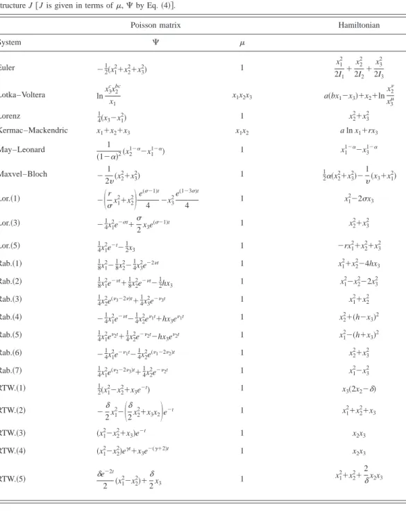
TABLE I. Examples of Hamiltonian systems given in the text. In each example we give a Hamiltonian H and a Poisson structure J关J is given in terms of␮,⌿ by Eq. 共4兲兴.

Poisson matrix Hamiltonian

System ⌿ ␮ Euler _⫺1 2共x1 2_⫹x 2 2_⫹x 3 2_{兲 1} x1 2 2I1⫹ x2 2 2I2⫹ x3 2 2I3 Lotka–Voltera lnx3 c x2 bc x1 x1x2x3 a共bx1⫺x3兲⫹x2⫹ln x2␯ x3␮ Lorenz 1_4共x3⫺x12_{兲 1 x} 2 2_⫹x 3 2 Kermac–Mackendric x1⫹x2⫹x3 x1x2 a ln x1⫹rx3 May–Leonard 1 共1⫺␣兲2共x2 1⫺␣_⫺x 1 1⫺␣_{兲 1 x} 1 1⫺␣_⫺x 3 1⫺␣ Maxvel–Bloch _⫺1 2␷共x2 2 ⫹x3 2_{兲 1} 1 2␣共x2 2 ⫹x3 2_兲⫺1 ␷共x3⫹x1 2_兲 Lor.共1兲 _⫺

冉

r ␴x1 2 ⫹x2 2

冊

e (␴⫺1)t 4 ⫺x3 2e (1⫺3␴)t 4 1 x1 2_⫺2␴ x3 Lor.共3兲 _⫺1 4x1 2_e⫺␴t_⫹␴ 2x3e (␴⫺1)t 1 x2 2 ⫹x3 2 Lor.共5兲 1 4x1 2 e⫺t⫺12x3 1 ⫺rx1 2_⫹x 2 2_⫹x 3 2 Rab.共1兲 1 8x1 2 ⫺1 8x2 2 ⫺1 4x3 2 e⫺2␯t 1 x1 2_⫹x 2 2_⫺4hx 3 Rab.共2兲 1 8x1 2_e⫺␯t_⫹1 8x2 2_e⫺␯t_⫺1 2hx3 1 x1 2 ⫺x2 2 ⫺2x3 2 Rab.共3兲 1 4x2 2_e(␯3⫺2␯)t⫹1 4x3 2_e⫺␯3t 1 x₁2⫹x₂2 Rab.共4兲 _⫺1 4x1 2 e⫺␯t⫺14x2 2 e␯1t⫹hx 3e␯1t 1 x2 2_⫹共h⫺x 3兲 2 Rab.共5兲 1 4x1 2 e␯2t⫹1 4x2 2 e⫺␯2t⫺hx 3e␯2 t _{1 x} 1 2 ⫺共h⫹x3兲2 Rab.共6兲 _⫺1 4x1 2_e⫺␯1t⫺1 4x2 2_e(␯1⫺2␯2)t 1 x₂2⫹x₃2 Rab.共7兲 1 4x1 2 e(␯2⫺2␯3)t⫹1 4x2 2 e⫺␯2t 1 x₁2⫺x₃2 RTW.共1兲 1 2共x1 2_⫺x 2 2_⫹x 3e⫺t兲 1 x3共2x2⫺␦兲 RTW.共2兲 _⫺␦ 2x1 2_⫺

冉

␦ 2x2 2_⫹x 3x2

冊

e⫺t 1 x1 2 ⫹x2 2 ⫹x3 RTW.共3兲 共x1 2 ⫺x2 2 ⫹x3兲e⫺t 1 x2x3 RTW.共4兲 共x1 2_⫺x 2 2_兲e␥t_⫹x 3e⫺(␥⫹2)t 1 x2x3 RTW.共5兲 ␦e ⫺2t 2 共x1 2_⫺x 2 2_兲⫹␦ 2x3 1 x1 2_⫹x 2 2_⫹2 ␦x2x3

V. CONCLUSION

We considered the Jacobi equation for the case N⫽3. We have found the most general Poisson

structure J in the neighborhood of regular points. This form is quite suitable for the study of the multi-Hamiltonian structure of the system. We found all possible compatible Poisson structures and corresponding bi-Hamiltonian systems. We studied our solution in the neighborhood of the irregular points of the Poisson structure and showed that it keeps its form. As an application of our

results we gave several examples which were reported earlier8 –15as bi-Hamiltonian systems. In

these examples we give the Casimirs, components of the Poisson matrix, the reduced equations and irregular points. Among all examples that we observed, only the Lotka–Voltera system has a special position. Our solution is not valid in the neighborhood of irregular points for this system. On the other hand the Hamiltonian function is not defined at such points as well. Hence the Lotka–Voltera equation does not have the Hamiltonian formulation in the neighborhood of such points.

ACKNOWLEDGMENTS

We would like to thank Dr. J. Grabowski and Dr. G. Marmo for drawing our attention to their

work.3 We thank to Dr. P. Olver for his constructive criticisms. We also thank the referee for

several suggestions. This work was partially supported by the Scientific and Technical Research Council of Turkey and by the Turkish Academy of Sciences.

1_{B. Hernandez-Bermejo, J. Math. Phys. 42, 4984共2001兲.} 2

B. Hernandez-Bermejo, Phys. Lett. A 287, 371共2001兲.

3_{J. Grabowski, G. Marmo, and A. M. Perelomov, Mod. Phys. Lett. A 8, 1719共1993兲.}

4_{P. J. Olver, Applications of Lie Groups to Differential Equations, Graduate Text in Mathematics, 2nd ed.} 共Springer-Verlag, New York, 1993兲, Vol. 107.

5

M. Blaszak, Multi-Hamiltonian Theory of Dynamical Systems, Text and Monographs in Physics共Springer-Verlag, New York, 1998兲.

6_{B. Hernandez-Bermejo and V. Fairen, Phys. Lett. A 234, 35共1997兲.} 7_{B. Hernandez-Bermejo and V. Fairen, J. Math. Phys. 39, 6162共1997兲.} 8_{X. Gu¨mral and Y. Nutku, J. Math. Phys. 34, 5691共1993兲.}

9

Y. Nutku, J. Phys. A 145, 27共1990兲. 10_{Y. Nutku, Phys. Lett. A 23, L1145共1990兲.}

11_{M. Baszak and S. Wojciechowski, Physica A 155, 545共1989兲.}

12_{J. Goedert, F. Haas, D. Huat, M. R. Feix, and L. Coiro, J. Phys. A 27, 6495共1994兲.} 13

E. N. Lorenz, J. Atmos. Sci. 27, 130共1963兲. 14

A. S. Pikovski and M. I. Rabinovich, Math. Phys. Rev. 2, 165共1981兲. 15_{T. C. Bountis, M. Bierand, and J. Hijmans, Phys. Lett. A 97, 11共1983兲.}