Role of the environmental spectrum in the decoherence and dephasing
of multilevel quantum systems
T. Hakioğlu and Kerim Savran
Department of Physics, Bilkent University, Bilkent, 06800 Ankara, Turkey 共Received 25 October 2004; published 25 March 2005兲
We examine the effect of multilevels on decoherence and dephasing properties of a quantum system con-sisting of a nonideal two level subspace, identified as the qubit, and a finite set of higher energy levels above this qubit subspace. The whole system is under interaction with an environmental bath through a Caldeira-Leggett type coupling. The model that we use is an rf-SQUID under macroscopic quantum coherence and coupled inductively to a flux noise characterized by an environmental spectrum. The model interaction can generate dipole couplings which can be appreciable between the qubit and the high levels. The decoherence properties of the qubit subspace is examined numerically using the master equation formalism of the system’s reduced density matrix. We calculate the relaxation and dephasing times as the spectral parameters of the environment are varied. We observe that, these calculated time scales receive contribution from all available frequencies in the noise spectrum 共even well above the system’s resonant frequency scales兲 stressing the dominant role played by the nonresonant transitions. The relaxation and dephasing and the leakage times thus calculated, strongly depend on the appreciably interacting levels determined by the strength of the dipole coupling. Under the influence of these nonresonant and multilevel effects, the validity of the two level ap-proximation is dictated not by the low temperature as conveniently believed, but by these multilevel dipole couplings as well as the availability of the environmental modes.
DOI: 10.1103/PhysRevB.71.115115 PACS number共s兲: 72.90.⫹y, 03.65.Yz, 03.67.Lx, 85.25.Dq I. INTRODUCTION
Currently a large number of model approaches are present for formulating the decoherence phenomena in the literature. The original Caldeira-Leggett model1is based on a quantum
system under the influence of a double well tunneling poten-tial with a linear coupling to an infinite bath of harmonic oscillators. If the potential is sufficiently smooth and the separation between the qubit and the high energy levels is well above the environmental temperature, this original model is normally represented as a two level system2共2LS兲
interacting with the bosonic environment 共spin-boson model兲. An incomplete list of this wide literature is provided in Refs. 3–5. Another popular model of decoherence is the central spin system in which central 2LS couples to a large number of environmental two level systems. The pros and cons of these two rival models have been extensively studied.5
Realistically, and aside from the genuine 2LS, a large ma-jority of physical systems suggested as qubit is far from be-ing ideal and include some number of higher energy levels. Higher levels in a multileveled system共MLS兲 can be effec-tive in the dynamics in two ways. The first is the leakage of the information from qubit subspace to higher levels which can happen in the presence of some uncontrollable coupling to a noise field with a sufficiently wide spectrum. Populating higher levels is basically thought to be a manifestation of resonant transitions at long times. On the other hand, for an arbitrary and wide noise spectrum, the same type of system-noise coupling can also induce nonresonant transitions which affect the short time dynamics of the interaction and contrib-ute to the decoherence times. In the coupling of a multi-leveled system to a wide environmental spectrum both ef-fects should therefore be expected. As a consequence of
these physical effects, and including the leakage factor, the validity of the analytic techniques devised to approximate these MLS in terms of simpler two-level model may become critically questionable.
In this work, we look for the answers of the following basic questions: 共a兲 Can one understand the effect of the higher levels on decoherence in a MLS under interaction with an environment? and共b兲 what is the role played by the environmental spectrum in the two-leveledness of a MLS?
The MLS can itself be manifestly N-leveled or a truncated approximation of a larger system with much higher number of levels. Examples of both cases have been well known. For the former, organic molecules with certain discrete rotational symmetries and low energy configurations of single polymer-ized chains are good examples. The vibrational energy spec-tra of atoms and molecules are good examples for the latter. We remark however, that a concise treatment of the decoher-ence effects based on such MLS has not been developed yet. Realistic MLS can be found for instance in superconducting systems in the macroscopic quantum coherence regimes. In this work, we use an rf-SQUID in the flux regime to generate our model system Hamiltonian for a multileveled quantum system. In the interaction with an environmental noise we use two scales which parametrize the low and high frequency sectors of the noise spectrum.
In Sec. II we give an introduction of the model MLS. There we concentrate on the properties of the environmen-tally induced dipole matrix elements between the levels. Sec-tion III recalls the reduced density matrix 共RDM兲 master equation formalism and adopts it for the coupling of the MLS to the environment. The noise correlator and the system-noise kernel, are defined in Sec. III. The results are presented together with the calculations for pure 2LS共in Sec. III A兲 to allow a comparison with the earlier work. Most original results of the paper are included in Sec. III. The
MLS with three or higher levels are examined in Sec. III B separately for the cases N = 3, N = 4, and 4⬍N. There, we confirm the leakage effects and observe that the short time nonresonant transitions dominate the decoherence times. As a consequence of these short time effects, we demonstrate in Sec. III C that, nonresonant transitions introduce severe re-strictions in the validity of the two level approximation.
II. THE MODEL MULTILEVEL SYSTEM
The majority of the accepted methods 共particularly the influence functional兲 widely used in the literature is appli-cable to the two-leveled dynamics. The results are generally believed to be true for 2LS and at temperatures well below the energy separation of the qubit and the high levels.1,2Such two level approximations are tempting since they allow ex-plicit analytic expressions for the decoherence times as func-tions of the system’s parameters. Exact methods are also available on pure 2LS.4
If one does not take for granted the validity of such ap-proximations, a direct investigation of the MLS-environment interaction must be made. In a MLS a need for explicit de-pendence on number of levels and their mutual couplings arises. To keep these dependencies, we represent here the MLS in its eigenenergy basis.
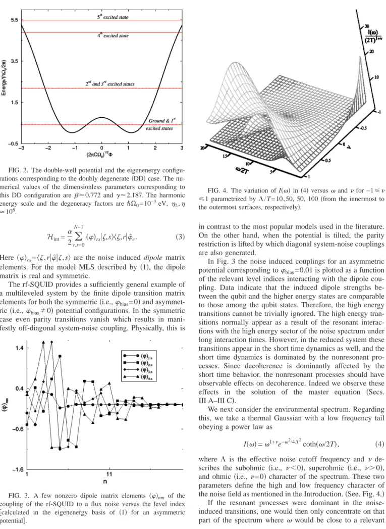
Our MLS is an rf-SQUID operating under macroscopic quantum coherence conditions given by the dimensionless Hamiltonian Hs/共ប⍀0兲 = 1 2关− 2 +共−bias兲2兴 +cos共␥兲, 共1兲
where⍀0= 2/
冑
LC is the harmonic frequency with L beingthe inductance of the SQUID loop and C is the effective capacitance of the Josephson junction,= EJ/ប⍀0 is the
di-mensionless ratio of the Josephson energy EJto the harmonic
energy,␥=ប冑L / C共2/⌽0兲2is a dimensionless scale
param-eter,bias= 2⌽bias/⌽0 is the effective bias in the flux
共ap-plicable in a current biased junction兲, and= 2⌽/共␥⌽0兲 is
the flux 共⌽兲 dependent dimensionless phase 共here ⌽0
= hc / 2e is the superconducting flux quantum兲. The Hamil-tonian共1兲 is clearly an infinite level system. Truncating the eigenspace at N levels, it becomes, in the energy basis
Hs=
兺
n=0 N−1En共兲兩,n典具,n兩, 共2兲
wheredescribes the set of system parameters⍀0,,␥,bias where En共兲, and 兩, n典 are, respectively, the parameter
de-pendent eigenenergies and eigenvectors of the MLS. This set of parameters is sufficiently general to accommodate a vari-ety of possible effects including the degeneracy of the lowest two levels 共the qubit subspace兲, the symmetry of the wave functions, etc. 关we define the degeneracy factor by =共E2
− E1兲/共E1− E0兲 for MLS and 2=共E1+ E0兲/共E1− E0兲 for
2LS兴. These parameters ⍀0,,biascontrol, respectively, the
high energy harmonic, the low energy anharmonic spectra and the reflection symmetry of the rf-SQUID potential, re-spectively. At low energies, a simple numerical diagonaliza-tion of共1兲 reveals that there are low lying eigenenergy
con-figurations within the double well regime in which the SQUID potential is strongly anharmonic. An interesting case here is to find highly degenerate6levels corresponding to the
first two eigenstates for the symmetric double-well potential 共i.e.,bias= 0兲. This particular case has been extensively
ex-amined previously for 2LS using semiclassical methods with an arbitrarily weak tunneling between the wells.2,3Another
configuration that turns out to be important in our calcula-tions is the doubly degenerate 共DD兲 configuration for sys-tems with 4艋N in which the first four levels are pairwise degenerate with large degeneracy factors. The double-well potential and energies corresponding to both SD and DD configurations which are often used in the paper, are shown in Figs. 1 and 2, respectively.
The rf-SQUID is shown to be a convenient 共and nonu-nique兲 model for studying multilevel effects due to the fact that the transitional dipole couplings between the qubit sub-space and the higher levels are non-negligible as shown in Fig. 3. Any other physical Hamiltonian with similar features would qualify for a model MLS.
In the rest of the paper the harmonic frequency ⍀0
= 2/
冑
LC is a free parameter that we use for scaling energy and time.6Coupling to noise: The system-noise interaction is consid-ered to be of Caldeira-Leggett type linear coupling between the SQUID’s macroscopic fluxˆ and the environmental flux
ˆe arising from the finite inductance of the SQUID loop. This coupling can be expanded in terms of the environmental modes asˆe=兺kk共bˆ−k
† + bˆ
k兲 where k is the mode index. The
system noise interaction is simplyHint=共␣/ 2兲ˆˆewhere ␣ represents the strength of the inductive coupling共␣ is to be normalized byប⍀0兲. The interaction Hamiltonian is given by
FIG. 1. The double-well potential and the eigenenergy configu-rations corresponding to the singly degenerate共SD兲 case. Here the numerical values of the dimensionless parameters for this SD con-figuration are⯝1.616 and ␥⯝1.753. The harmonic energy scale and the degeneracy factors are, respectively, ប⍀0= 10−3eV and 2⯝107.
Hint=␣ 2r,s=0
兺
N−1
共兲rs兩,s典具,r兩ˆe. 共3兲
Here共兲rs=具, r兩ˆ兩, s典 are the noise induced dipole matrix
elements. For the model MLS described by 共1兲, the dipole matrix is real and symmetric.
The rf-SQUID provides a sufficiently general example of a multileveled system by the finite dipole transition matrix elements for both the symmetric共i.e.,bias= 0兲 and
asymmet-ric共i.e.,bias⫽0兲 potential configurations. In the symmetric
case even parity transitions vanish which results in mani-festly off-diagonal system-noise coupling. Physically, this is
in contrast to the most popular models used in the literature. On the other hand, when the potential is tilted, the parity restriction is lifted by which diagonal system-noise couplings are also generated.
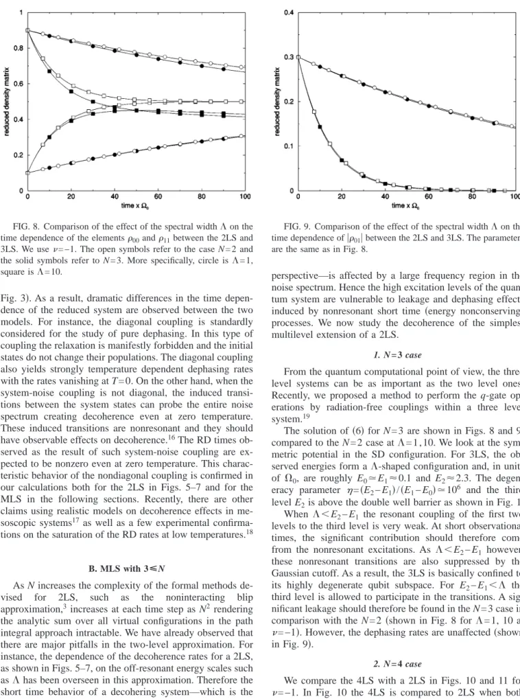
In Fig. 3 the noise induced couplings for an asymmetric potential corresponding tobias= 0.01 is plotted as a function
of the relevant level indices interacting with the dipole cou-pling. Data indicate that the induced dipole strengths be-tween the qubit and the higher energy states are comparable to those among the qubit states. Therefore, the high energy transitions cannot be trivially ignored. The high energy tran-sitions normally appear as a result of the resonant interac-tions with the high energy sector of the noise spectrum under long interaction times. However, in the reduced system these transitions appear in the short time dynamics as well, and the short time dynamics is dominated by the nonresonant pro-cesses. Since decoherence is dominantly affected by the short time behavior, the nonresonant processes should have observable effects on decoherence. Indeed we observe these effects in the solution of the master equation 共Secs. III A–III C兲.
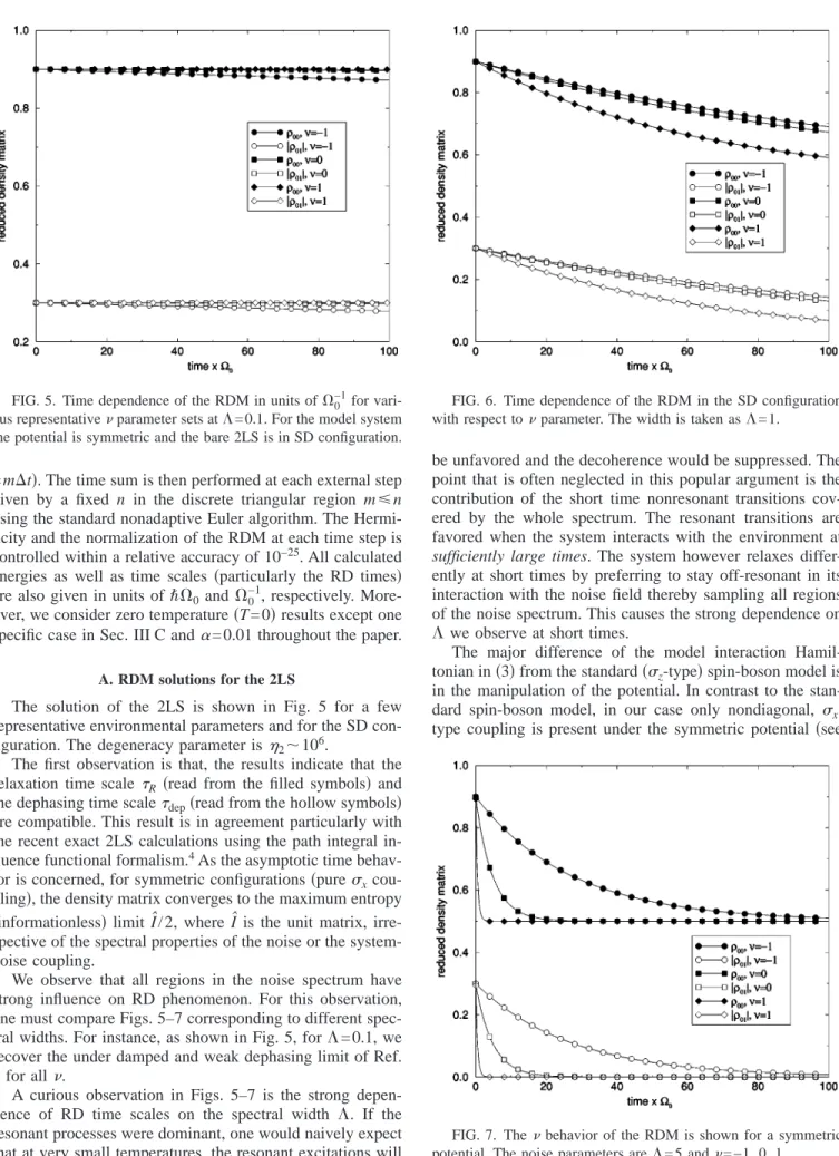
We next consider the environmental spectrum. Regarding this, we take a thermal Gaussian with a low frequency tail obeying a power law as
I共兲 =1+e−2/4⌳2coth共/2T兲, 共4兲 where ⌳ is the effective noise cutoff frequency and de-scribes the subohmic 共i.e., ⬍0兲, superohmic 共i.e., ⬎0兲, and ohmic共i.e., = 0兲 character of the spectrum. These two parameters define the high and low frequency character of the noise field as mentioned in the Introduction.共See. Fig. 4.兲 If the resonant processes were dominant in the noise-induced transitions, one would then only concentrate on that part of the spectrum where would be close to a relevant FIG. 2. The double-well potential and the eigenenergy
configu-rations corresponding to the doubly degenerate共DD兲 case. The nu-merical values of the dimensionless parameters corresponding to this DD configuration are⯝0.772 and ␥⯝2.187. The harmonic energy scale and the degeneracy factors are ប⍀0= 10−3eV, 2, ⯝106.
FIG. 3. A few nonzero dipole matrix elements 共兲nm of the
coupling of the rf-SQUID to a flux noise versus the level index 关calculated in the eigenenergy basis of 共1兲 for an asymmetric potential兴.
FIG. 4. The variation of I共兲 in 共4兲 versus and for −1艋 艋1 parametrized by ⌳/T=10,50, 50, 100 共from the innermost to the outermost surfaces, respectively兲.
transition energy⌬E. For −1ⱗ 共subohmic兲, the following two regions are of particular importance:共a兲 at sufficiently low temperatures and high cutoff corresponding to TⰆ⌳, the dominant mechanism of relaxation is through spontaneous de-excitations,7we call this region region-I;共b兲 at high
tem-peratures and high cutoff the regionⰆmin共⌳,T兲 provides a wider range of strong environmental couplings which we call region II. If the character of the spectrum is more like ohmic or superohmic, i.e., ⯝0 or ⯝1, respectively, the availability of the low frequency modes is not so high. Therefore, in the ohmic and superohmic regimes, region II would dominate the relaxation/dephasing 共RD兲 phenomena. Hence it is concluded that, if the resonant processes were dominant, one would maintain a sufficiently low environ-mental temperature to largely eliminate the decoherence ef-fects for ohmic and superohmic cases.
Our calculations in this work however demonstrate that decoherence cannot be avoided at zero temperature and the decoherence times are influenced not by the strength of the spectral coupling at the resonant transitions but by the whole spectral range.
III. MASTER EQUATION AND THE REDUCED DENSITY MATRIX FOR THE MLS
In the study of decoherence due to the weak environmen-tal influence, one conventional way is to calculate the time dependent RDM by solving the master equation. This for-malism has been known since the works of Bloch, Redfield, and Fano共BRF兲8and widely applied to the current decoher-ence problems for which many standard referdecoher-ences exist.9
The standard BRF formalism assumes fully Markovian con-ditions for the solution of the master equation, which leads to analytically solvable results for 2LS.10 However, this
as-sumption is not free of drawbacks which was explored origi-nally in Ref. 11 and lately in Ref. 12 as well as in Ref. 13 in the context of spin magnetic resonance and relaxation.
The time evolution of the RDM is obtained by − iបd
dt˜ˆ共t兲 = 关˜ˆ共t兲,H ˜
int共t兲兴, 共5兲
where the tilde denotes the interaction picture. In the context of decoherence, we will give more emphasis on the exponen-tial time scales in the solution of共5兲. A convenient way to proceed is then to apply the Born-Oppenheimer approxima-tion in which the full density matrix is initially a product of the system and environmental ones 关i.e., ˜ˆ共0兲=˜ˆ共S兲共0兲 丢˜ˆe共0兲兴 and at any later and sufficiently short time approxi-mately separates as˜ˆ共t兲=˜ˆ共S兲共t兲丢˜ˆe共0兲.
The iterative solution of共5兲 including the second order in the interaction with the partial trace performed over the en-vironmental degrees of freedom yields the master equation for the RDM, d dt˜nm 共S兲共t兲 = −
冕
0 t dt⬘
兺
r,s Krsnm共t,t⬘
兲˜rs共S兲共t⬘
兲, 共6兲 in which we adopt the model interaction Hamiltonian共3兲 for the system-noise kernel. This kernel is found to beKrsnm共t,t
⬘
兲 =␣2
4 兵F共t − t
⬘
兲关共˜ˆt˜ˆt⬘兲nr␦s,m−共˜ˆt⬘兲nr共˜ˆt兲sm兴 +F * 共t − t⬘
兲关共˜ˆt⬘˜ˆt兲ms␦r,n−共˜ˆt兲nr共˜ˆt⬘兲sm兴其.共7兲 HereF共t−t
⬘
兲=F*共t⬘
− t兲 is the complex noise correlation function, F共t − t⬘
兲 = Tre关˜ˆe共t兲˜ˆe共t⬘
兲e共0兲兴 = 具˜ˆe共t兲˜ˆe共t⬘
兲典 共8兲 and ˜ˆt=兺
k,ᐉ=0 N−1共ˆ兲kᐉe−i共Ek−Eᐉ兲t兩,k典具,ᐉ兩 共9兲
is the dipole operator in the interaction picture. Expanding the noise field ˆe in the independent harmonic modes and calculating共8兲 in thermal equilibrium one obtains the stan-dard thermal noise correlator,
F共t − t
⬘
兲 = 2兺
k k 2关coth共 k/2T兲cosk共t − t⬘
兲 − i sink共t − t⬘
兲兴. 共10兲 The noise spectrum is assumed to be continuous of which the real part is responsible for RD effects and is given by the spectral density in 共4兲. In the numerical calculations we in-clude the noise correlation function as15F共t − t
⬘
兲 = 2冕
0
⬁
d1+e−2/4⌳2关coth共/2T兲cos共t − t
⬘
兲− i sin共t − t
⬘
兲兴. 共11兲Inserting共11兲 in 共7兲 we obtain the system-noise kernel for our model. A numerical upper frequency cutoff of max = 5⌳ is used in the numerical integral in 共11兲.
The solution of 共6兲 is determined in the weak system-noise interaction limit by the competition of three time scales:B, noise correlation time scale,RandD, the
relax-ation and dephasing time scales14 of the reduced system,
respectively. The noise correlation time scale is found roughly from the thermal Gaussian bath spectral width as
B⯝1/⌳. The RD time scales are found by fitting the
enve-lope in the solution of共6兲 to the decaying exponential3
兩ij共t兲兩 ⯝ 兩ij共⬁兲兩 + 关兩ij共0兲兩 − 兩ij共⬁兲兩兴exp共− t/ij兲, 共12兲 by the formula ij −1⯝ − 1 1 −兩ij共⬁兲/ij共0兲兩
冏
d ln兩ij兩 dt冏
t=0, 共13兲 where in共12兲 and 共13兲, i= j=1 is used in the calculation of the relaxation rate共R−1兲 and i=0, j=1 is used for the qubit dephasing rate 共D−1兲. For the RDM at asymptotic times we have11共⬁兲=1/N and 兩10共⬁兲兩=0. The equation 共13兲 breaksdown when 兩ij共0兲兩=兩ij共⬁兲兩 which we stay away from by
appropriately choosingij共0兲.
In this work, the numerical solution of共6兲 is performed by discretizing time in steps of ⌬t=10−2⍀0−1 共i.e., t=n⌬t, t
⬘
= m⌬t兲. The time sum is then performed at each external step given by a fixed n in the discrete triangular region m艋n using the standard nonadaptive Euler algorithm. The Hermi-ticity and the normalization of the RDM at each time step is controlled within a relative accuracy of 10−25. All calculated energies as well as time scales 共particularly the RD times兲 are also given in units ofប⍀0 and⍀0−1, respectively. More-over, we consider zero temperature共T=0兲 results except one specific case in Sec. III C and␣= 0.01 throughout the paper.
A. RDM solutions for the 2LS
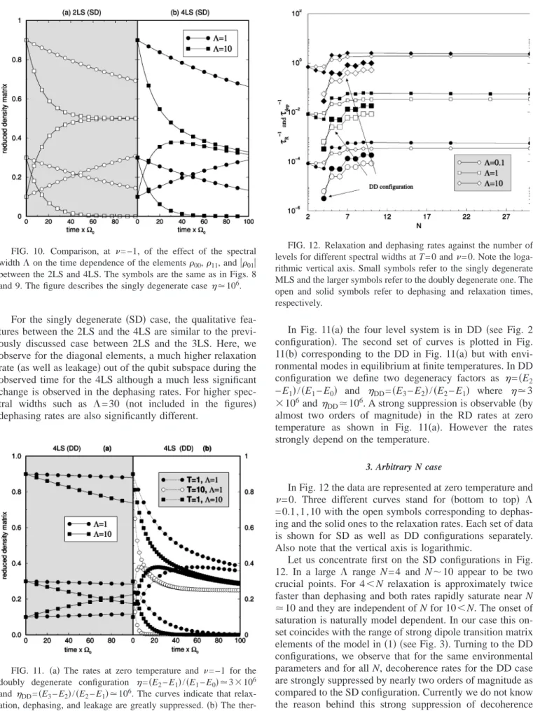
The solution of the 2LS is shown in Fig. 5 for a few representative environmental parameters and for the SD con-figuration. The degeneracy parameter is2⬃106.
The first observation is that, the results indicate that the relaxation time scale R 共read from the filled symbols兲 and
the dephasing time scaledep共read from the hollow symbols兲
are compatible. This result is in agreement particularly with the recent exact 2LS calculations using the path integral in-fluence functional formalism.4As the asymptotic time
behav-ior is concerned, for symmetric configurations共purex
cou-pling兲, the density matrix converges to the maximum entropy 共informationless兲 limit Iˆ/2, where Iˆ is the unit matrix, irre-spective of the spectral properties of the noise or the system-noise coupling.
We observe that all regions in the noise spectrum have strong influence on RD phenomenon. For this observation, one must compare Figs. 5–7 corresponding to different spec-tral widths. For instance, as shown in Fig. 5, for⌳=0.1, we recover the under damped and weak dephasing limit of Ref. 3 for all.
A curious observation in Figs. 5–7 is the strong depen-dence of RD time scales on the spectral width ⌳. If the resonant processes were dominant, one would naively expect that at very small temperatures, the resonant excitations will
be unfavored and the decoherence would be suppressed. The point that is often neglected in this popular argument is the contribution of the short time nonresonant transitions cov-ered by the whole spectrum. The resonant transitions are favored when the system interacts with the environment at sufficiently large times. The system however relaxes differ-ently at short times by preferring to stay off-resonant in its interaction with the noise field thereby sampling all regions of the noise spectrum. This causes the strong dependence on ⌳ we observe at short times.
The major difference of the model interaction Hamil-tonian in共3兲 from the standard 共z-type兲 spin-boson model is
in the manipulation of the potential. In contrast to the stan-dard spin-boson model, in our case only nondiagonal, x,
type coupling is present under the symmetric potential共see FIG. 5. Time dependence of the RDM in units of⍀0−1for
vari-ous representative parameter sets at ⌳=0.1. For the model system the potential is symmetric and the bare 2LS is in SD configuration.
FIG. 6. Time dependence of the RDM in the SD configuration with respect to parameter. The width is taken as ⌳=1.
FIG. 7. The behavior of the RDM is shown for a symmetric potential. The noise parameters are⌳=5 and=−1, 0, 1.
Fig. 3兲. As a result, dramatic differences in the time depen-dence of the reduced system are observed between the two models. For instance, the diagonal coupling is standardly considered for the study of pure dephasing. In this type of coupling the relaxation is manifestly forbidden and the initial states do not change their populations. The diagonal coupling also yields strongly temperature dependent dephasing rates with the rates vanishing at T = 0. On the other hand, when the system-noise coupling is not diagonal, the induced transi-tions between the system states can probe the entire noise spectrum creating decoherence even at zero temperature. These induced transitions are nonresonant and they should have observable effects on decoherence.16The RD times
ob-served as the result of such system-noise coupling are ex-pected to be nonzero even at zero temperature. This charac-teristic behavior of the nondiagonal coupling is confirmed in our calculations both for the 2LS in Figs. 5–7 and for the MLS in the following sections. Recently, there are other claims using realistic models on decoherence effects in me-soscopic systems17 as well as a few experimental confirma-tions on the saturation of the RD rates at low temperatures.18
B. MLS with 3ÏN
As N increases the complexity of the formal methods de-vised for 2LS, such as the noninteracting blip approximation,3increases at each time step as N2rendering
the analytic sum over all virtual configurations in the path integral approach intractable. We have already observed that there are major pitfalls in the two-level approximation. For instance, the dependence of the decoherence rates for a 2LS, as shown in Figs. 5–7, on the off-resonant energy scales such as⌳ has been overseen in this approximation. Therefore the short time behavior of a decohering system—which is the most prominent regime in the quantum computational
perspective—is affected by a large frequency region in the noise spectrum. Hence the high excitation levels of the quan-tum system are vulnerable to leakage and dephasing effects induced by nonresonant short time 共energy nonconserving兲 processes. We now study the decoherence of the simplest multilevel extension of a 2LS.
1. N = 3 case
From the quantum computational point of view, the three level systems can be as important as the two level ones. Recently, we proposed a method to perform the q-gate op-erations by radiation-free couplings within a three level system.19
The solution of共6兲 for N=3 are shown in Figs. 8 and 9, compared to the N = 2 case at⌳=1,10. We look at the sym-metric potential in the SD configuration. For 3LS, the ob-served energies form a⌳-shaped configuration and, in units of ⍀0, are roughly E0⯝E1⬇0.1 and E2⬇2.3. The degen-eracy parameter =共E2− E1兲/共E1− E0兲⯝106 and the third
level E2is above the double well barrier as shown in Fig. 1.
When ⌳⬍E2− E1 the resonant coupling of the first two
levels to the third level is very weak. At short observational times, the significant contribution should therefore come from the nonresonant excitations. As ⌳⬍E2− E1 however,
these nonresonant transitions are also suppressed by the Gaussian cutoff. As a result, the 3LS is basically confined to its highly degenerate qubit subspace. For E2− E1⬍⌳ the
third level is allowed to participate in the transitions. A sig-nificant leakage should therefore be found in the N = 3 case in comparison with the N = 2 共shown in Fig. 8 for ⌳=1, 10 at
= −1兲. However, the dephasing rates are unaffected 共shown in Fig. 9兲.
2. N = 4 case
We compare the 4LS with a 2LS in Figs. 10 and 11 for
= −1. In Fig. 10 the 4LS is compared to 2LS when both systems are in SD configuration.
FIG. 8. Comparison of the effect of the spectral width⌳ on the time dependence of the elements00and11between the 2LS and 3LS. We use=−1. The open symbols refer to the case N=2 and the solid symbols refer to N = 3. More specifically, circle is⌳=1, square is⌳=10.
FIG. 9. Comparison of the effect of the spectral width⌳ on the time dependence of兩01兩 between the 2LS and 3LS. The parameters are the same as in Fig. 8.
For the singly degenerate共SD兲 case, the qualitative fea-tures between the 2LS and the 4LS are similar to the previ-ously discussed case between 2LS and the 3LS. Here, we observe for the diagonal elements, a much higher relaxation rate共as well as leakage兲 out of the qubit subspace during the observed time for the 4LS although a much less significant change is observed in the dephasing rates. For higher spec-tral widths such as ⌳=30 共not included in the figures兲 dephasing rates are also significantly different.
In Fig. 11共a兲 the four level system is in DD 共see Fig. 2 configuration兲. The second set of curves is plotted in Fig. 11共b兲 corresponding to the DD in Fig. 11共a兲 but with envi-ronmental modes in equilibrium at finite temperatures. In DD configuration we define two degeneracy factors as =共E2 − E1兲/共E1− E0兲 and DD=共E3− E2兲/共E2− E1兲 where ⯝3 ⫻106and
DD⯝106. A strong suppression is observable共by
almost two orders of magnitude兲 in the RD rates at zero temperature as shown in Fig. 11共a兲. However the rates strongly depend on the temperature.
3. Arbitrary N case
In Fig. 12 the data are represented at zero temperature and
= 0. Three different curves stand for 共bottom to top兲 ⌳ = 0.1, 1 , 10 with the open symbols corresponding to dephas-ing and the solid ones to the relaxation rates. Each set of data is shown for SD as well as DD configurations separately. Also note that the vertical axis is logarithmic.
Let us concentrate first on the SD configurations in Fig. 12. In a large ⌳ range N=4 and N⬃10 appear to be two crucial points. For 4⬍N relaxation is approximately twice faster than dephasing and both rates rapidly saturate near N ⯝10 and they are independent of N for 10⬍N. The onset of saturation is naturally model dependent. In our case this on-set coincides with the range of strong dipole transition matrix elements of the model in共1兲 共see Fig. 3兲. Turning to the DD configurations, we observe that for the same environmental parameters and for all N, decoherence rates for the DD case are strongly suppressed by nearly two orders of magnitude as compared to the SD configuration. Currently we do not know the reason behind this strong suppression of decoherence rates in doubly degenerate systems.
FIG. 10. Comparison, at =−1, of the effect of the spectral width⌳ on the time dependence of the elements00,11, and兩01兩 between the 2LS and 4LS. The symbols are the same as in Figs. 8 and 9. The figure describes the singly degenerate case⯝106.
FIG. 11. 共a兲 The rates at zero temperature and =−1 for the doubly degenerate configuration =共E2− E1兲/共E1− E0兲⯝3⫻106
andDD=共E3− E2兲/共E2− E1兲⯝106. The curves indicate that
relax-ation, dephasing, and leakage are greatly suppressed.共b兲 The ther-mal case at the indicated⌳, T values at=−1.
FIG. 12. Relaxation and dephasing rates against the number of levels for different spectral widths at T = 0 and=0. Note the loga-rithmic vertical axis. Small symbols refer to the singly degenerate MLS and the larger symbols refer to the doubly degenerate one. The open and solid symbols refer to dephasing and relaxation times, respectively.
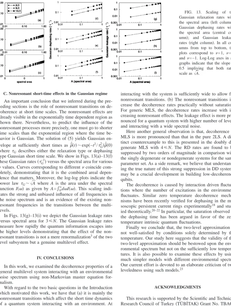
C. Nonresonant short-time effects in the Gaussian regime An important conclusion that we inferred during the pre-ceding sections is the role of nonresonant transitions on de-coherence at short time scales. The nonresonant effects are already visible in the exponentially time dependent region as shown there. Nevertheless, to predict the influence of the nonresonant processes more precisely, one must go to shorter time scales than the exponential region where the time be-havior is Gaussian. The solution of共5兲 yields Gaussian en-velope at sufficiently short times as˜ˆ共t兲⬃exp共−t2/
G
2兲
˜ˆ共0兲 whereG describes either the relaxation type or dephasing
type Gaussian short time scale. We show in Figs. 13共a兲–13共f兲 these Gaussian rates共G−1兲 versus the spectral area for various
values. Curves corresponding to different coincide com-pletely, demonstrating that it is the combined areal depen-dence that matters. Moreover, the log-log plots indicate the power law G⬃
冑
A where A is the area under the spectralfunction I共兲 as given by A=兰0⬁dI共兲. This scaling indi-cates the strong and unbiased influence of all frequencies in the noise spectrum and is an evidence of the existing non-resonant frequencies in the transitions between the multi-levels.
In Figs. 13共g兲–13共i兲 we depict the Gaussian leakage rates versus spectral area for 3艋N. The Gaussian leakage rates measure how rapidly the quantum information escapes into the higher levels demonstrating that the effect of the non-resonant transitions is not a mere renormalization3of the two
level subsystem but a genuine multilevel effect.
IV. CONCLUSIONS
In this work, we examined the decoherence properties of a general multilevel system interacting with an environmental noise spectrum using non-Markovian master equation for-malism.
With regard to the two basic questions in the Introduction which motivated this work, we have that共a兲 it is mainly the nonresonant transitions which affect the short time dynamics of a quantum system interacting with an environment. At short observation times, the multileveledness is unavoidable if there is finite coupling between the levels; and, if the noise
interacting with the system is sufficiently wide to allow for nonresonant transitions. 共b兲 The nonresonant transitions in-crease the decoherence rates practically without saturation. For generic MLS, the decoherence rates increase with in-creasing nonresonant effects. The leakage effect is more pro-nounced for a quantum system with higher number of levels and interacting with a wide spectral noise.
Here another general observation is that, decoherence in MLS is more pronounced than that in the pure 2LS. A dis-tinct counterexample to this is presented in the doubly de-generate MLS with 4艋N. The RD rates are found to be suppressed by two orders of magnitude in comparison with the singly degenerate or nondegenerate systems for the same parameter set. As a side remark, we believe that understand-ing the true nature of this strong suppression in DD systems may be a crucial development in building low-decoherence qubits.
The decoherence is caused by interaction driven fluctua-tions where the number of excitafluctua-tions in the environment fluctuates. Similar zero temperature decoherence mecha-nisms have been recently verified for dephasing in the me-soscopic persistent current rings experimentally18 and stud-ied theoretically.20–22In particular, the saturation observed in
the dephasing time has been argued in favor of the zero temperature intrinsic quantum fluctuations.
Finally we conclude that, the two-level approximation is not well-satisfied by conditions solely determined by the temperature. Our study here suggests that the validity of the two-level approximation should be bestowed upon the envi-ronmental spectrum but not on the sufficiently low tempera-tures. It is also possible to examine these effects by using much simpler models with different environmental spectra. Our current effort is devoted to an elaborate criticism of two leveledness using such models.23
ACKNOWLEDGMENTS
This research is supported by the Scientific and Technical Research Council of Turkey共TÜBİTAK兲 Grant No. TBAG-2111共101T136兲. The authors thank I. O. Kulik and E. Mese for critical comments.
FIG. 13. Scaling of the Gaussian relaxation rates with the spectral area 共left column兲; Gaussian dephasing rates with the spectral area 共central col-umn兲; and Gaussian leakage rates 共right column兲. In all col-umns from top to bottom, the plots correspond to =1, =0, and =−1. Log-Log axes in all graphs indicate that the slope is 0.5 impliying that both rates scale as
冑
A.1A. O. Caldeira and A. J. Leggett, Phys. Rev. Lett. 46, 211共1981兲;
Ann. Phys.共N.Y.兲 149, 374 共1983兲.
2A. J. Leggett and Anupam Garg, Phys. Rev. Lett. 54, 857共1985兲. 3A. J. Leggett, S. Chakravarty, A. T. Dorsey, Matthew P. A. Fisher,
Anupam Garg, and W. Zwerger, Rev. Mod. Phys. 59, 1共1987兲; Daniel Loss and David P. DiVincenzo, Int. J. Mod. Phys. B 17, 5489 共2003兲; Till Vorrath, Tobias Brandes, and Bernhard Kramer, cond-mat/304118共unpublished兲.
4Charis Anastopoulos and B. L. Hu, Phys. Rev. A 62, 033821 共2000兲.
5M. Dube and P. C. E. Stamp, Quantum Physics of Open Systems 关Chem. Phys., Special issue 268, 257 共2001兲兴; cond-mat/ 0102156; P. C. E. Stamp and I. S. Tupitsyn, cond-mat/0308139; Leonid Fedichkin, Akrady Fedorov, and Vladimir Privman, Proc. SPIE 5105, 243共2003兲.
6In a finite double well potential there is no manifest degeneracy.
However highly degenerate configurations can be obtained in the vicinity of level crossings. It can be numerically shown关see for instance T. Hakioglu, J. Anderson, and F. Wellstood, Phys. Rev. B 66, 115324共2002兲兴 that at the level crossings the sym-metric and antisymsym-metric configurations are highly confined ei-ther within the left or the right wells. The tunneling matrix ele-ment is proportional to the overlap of these configurations which is minimized at the level crossings.
7We assume that the system is initially prepared at a given
super-position state 共0兲=a兩0典+b兩1典 where 兩0典 and 兩1典 are, respec-tively, the ground and the first excited states in the qubit sub-space.
8F. Bloch, Phys. Rev. 102, 104共1956兲; A. G. Redfield, IBM J.
Res. Dev. 1, 19共1957兲; U. Fano, Phys. Rev. 96, 869 共1954兲.
9Michele Governale, Milena Grifoni, and Gerd Shön, Chem. Phys.
208, 273共2001兲; Guido Burkard, Roger H. Koch, and David P. DiVincenzo, Phys. Rev. B 69, 064503共2004兲; Yuriy Makhlin, Gerd Schön, and Alexander Shnirman, New Dimensions in Me-soscopic Physics, edited by R. Fazio, V. F. Gantmakher, and Y.
Imry共Kluwer, Dordrecht, 2003兲, pp. 197–236
10Anatoly Yu. Smirnov, Phys. Rev. B 67, 155104共2003兲, and the
third reference in Ref. 9.
11P. N. Argyres and P. L. Kelley, Phys. Rev. 134, 98共1964兲. 12A. Suarez, R. Silbey, and I. Oppenheim, J. Chem. Phys. 97, 5101
共1992兲.
13M. Grifoni, E. Paladino, and U. Weiss, Eur. Phys. J. B 10, 719 共1999兲.
14H. P. Breuer and F. Petruccione, The Theory of Open Quantum
Systems共Oxford University Press, Oxford, 2002兲.
15B. L. Hu, Juan Pablo Paz, and Yuhong Zhang, Phys. Rev. D 45,
2843共1992兲.
16Florian Marquardt and C. Bruder, Phys. Rev. B 65, 125315 共2002兲.
17D. S. Golubev and A. D. Zaikin, Phys. Rev. Lett. 81, 1074 共1998兲; Phys. Rev. B 62, 14 061 共2000兲.
18P. Mohanty, E. M. Q. Jariwala, and R. A. Webb, Phys. Rev. Lett.
78, 3366共1997兲.
19I. O. Kulik and T. Hakioğlu, Eur. Phys. J. B 30, 219共2002兲; also
recently, a Markovian Linblad approach was used for the RDM of a multilevel system in connection with the quantum Zeno effect 关see for instance, D. Bruno, P. Facchi, S. Longo, P. Minelli, S. Pascazio, and A. Scardicchio, quant-ph/0206143 共un-published兲兴.
20D. Natelson, R. L. Willett, K. W. West, and L. N. Pfeiffer, Phys.
Rev. Lett. 86, 1821共2001兲.
21Pascal Cedraschi, Vadim V. Ponomarenko, and Markus Büttiker,
Phys. Rev. Lett. 84, 346共2000兲; M. Büttiker, Decoherence from Vacuum Fluctuations, Proc. Electronic Correlations: From Meso- to Nano-Physics, edited by G. Montambaux and T. Mar-tin共EDP Sciences, Les Ulis, 2001兲, pp. 231–236; see also cond-mat/0105519共unpublished兲.
22J. J. Lin and N. Giordano, Phys. Rev. B 35, 1071共1987兲; D. M.
Pookr et al., J. Phys.: Condens. Matter 1, 3289共1989兲.