YASAR UNIVERSITY
GRADUATE SCHOOL OF NATURAL AND APPLIED SCIENCES
MASTER THESIS
TRANSIENT VOLTAGE STABILITY ENHANCEMENT
OF AUTO PRODUCER POWER PLANT
Sedat LEBLEBİCİOĞLU
Thesis Advisor: Asst. Assoc. Dr. Hacer ŞEKERCİ
Department of Electrical and Electronics Engineering
Presentation Date: 17.10.2014
Bornova-İZMİR 2014
APPROVAL
This study, titled “TRANSIENT VOLTAGE STABILITY ENHANCEMENT OF AUTO PRODUCER POWER PLANT” and presented as Master (Post Graduate) Thesis by Sedat LEBLEBİCİOĞLU, has been evaluated in compliance with the relevant provisions of Y.U. Graduate Education and Training Regulations and Y.U. Institute of Science Education and Training Direction. The jury members below have decided for the defence of this thesis, and it has been declared by consensus / majority of votes that the candidate has succeeded in his thesis defence examination dated ………...
Jury Members: Signature:
Head : ………. ……….
Rapporteur Member : ………. ……….
ABSTRACT
TRANSIENT VOLTAGE STABILITY ENHANCEMENT OF AUTO PRODUCER POWER PLANT
LEBLEBİCİOĞLU, Sedat
MSc in Electrical and Electronics Engineering Thesis Advisor: Asst. Assoc. Dr. Hacer ŞEKERCİ
September 2014, 72 pages
The voltage stability is a major concern in power system operation. The power systems operated under stressed conditions and close to instability limits because of increasing power demand, this can initiates voltage instability lead to a system voltage collapse.
This study explains the enhancement of transient voltage stability of an auto producer power plant in an industrial zone. Critical points of transient voltage stability is discussed and the ways to enhance stability is investigated.
The power plant, electrical distribution system and the factories as loads are modeled and simulated within SINCAL (by SIEMENS) software. Several operational conditions like decoupling (islanding), load shedding and distribution system configuration change studied on these simulations. The conditions that lead to transient voltage instability and ways to overcome this problem are investigated. Primary focus is investigating the operational solutions without new investment on the existing power system.
ÖZET
OTOPRODÜKTÖR ENERJİ SANTRALI TRANZİENT GERİLİM KARARLILIĞININ ARTIRILMASI
LEBLEBİCİOĞLU, Sedat
Yüksek Lisans Tezi, Elektrik ve Elektronik Mühendisliği Bölümü Tez Danışmanı: Yard. Doç. Dr. Hacer ŞEKERCİ
Eylül 2014, 72 sayfa
Gerilim kararlılığı güç sistemi işletmesinde önemli bir husustur. Artan güç ihtiyacı nedeniyle güç sistemleri stres altında ve kararsızlık sınırına yakın çalışmakta, gerilim kararsızlığı tetiklenerek system gerilimi çökebilmektedir.
Bu çalışmada bir endüstri bölgesindeki otoprodüktör enerji tesisinin tranzient gerilim kararlılığının artırılması açıklanmaktadır. Tranzient gerilim kararlılığının önemli noktaları tartışılmış ve kararlılığı artırma yolları araştırılmıştır.
Enerji santralı, elektrik dağıtım sistemi ve fabrikalar yük şeklinde SINCAL (SIEMENS firmasına ait) yazılımında modellenerek simüle edilmiştir. Simülasyonlarda şebekeden ayrılma (adalaşma), yük atma ve dağıtım sistemi konfigürasyon değişikliği gibi çeşitli işletme şartları çalışılmıştır. Tranzient gerilim kararsızlığına neden olan şartlar ve bu problemi aşma yolları araştırılmıştır. Öncelikli hedef mevcut güç sisteminde yeni yatırım yapmadan işletimsel çözümlerin araştırılmasıdır.
ACKNOWLEDGMENTS
I would like to thank my advisor Asst. Assoc. Dr. Hacer ŞEKERCİ for her generosity, support, and inspiration. This thesis would not have been possible to accomplish without the help and guidance she has provided me throughout the entire process.
Last but not least, I would like to thank my family for their support given me while pursuing my masters.
TABLE OF CONTENTS
Page
ABSTRACT ...v
ÖZET ………...vii
ACKNOWLEDGEMENTS ...ix
INDEX OF FIGURES ...xiii
INDEX OF TABLES ...xv
INDEX OF SYMBOLS AND ABBREVIATIONS...xvi
1 INTRODUCTION ...1
1.1 Background ...1
1.2 Scope and Objective ...2
1.3 Organization of Thesis ...3
2 VOLTAGE STABILITY ...4
2.1 Definition and Classification of Voltage Stability...4
2.1.1 Definition and Classification of Voltage Stability by IEEE/CIGRE ...4
2.1.2 Definition and Classification of Voltage Stability by EPRI ...6
TABLE OF CONTENTS (cont’d)
Page
2.3 Literature Survey ...10
2.4 Voltage Stability Analysis Methods ...14
3 MODELING OF POWER SYSTEM ELEMENTS ...17
3.1 Load Model Category ...17
3.1.1 Static Load Model ...17
3.1.2 Dynamic Load Model ...17
3.1.3 Composite Load Model ...18
3.1.4 Voltage Instability & Induction Motor Stalling ...19
3.2 Load Torque Characteristic ...20
3.3 Governor Model …...21
3.4 Exciter Model ...24
4 SIMULATION ...27
4.1 Simulation Software ...27
4.2 Modeling of Industrial Cogeneration System ...28
TABLE OF CONTENTS (cont’d)
Page
5 CASE STUDIES ...32
5.1 Overview ...32
5.2 Simulation of Cases ...33
5.2.1 Case-1: Decoupling Time ...33
5.2.2 Case-2: Load Shedding After Decoupling ...39
5.2.3 Case-3: Power System Network Configuration ...45
6 DISCUSSION ...50
7 CONCLUSION ...52
8 SUGGESTIONS ...53
INDEX OF FIGURES
FIGURE Page
2.1 Classification of power system stability ... 5
2.2 Time frames for voltage instability ... 7
2.3 TVA and MLG&W power systems ... 8
2.4 Post disturbance system conditions ... 10
2.5 One-line diagram of the cogeneration system ... 12
2.6 Normalized P-V Curves ... 15
2.7 Normalized Q-V Curves ... 16
3.1 Induction motor torque/speed curve ... 19
3.2 Torque/speed curve of a typical load ... 20
3.3 Turbine-governor model IEEEG1 ... 22
3.4 Excitation system model IEEEX2 ... 25
4.1 Industrial cogeneration system ... 29
5.1 Industrial cogeneration system network configuration (154 kV & 34,5 kV) . 33 5.2 Case-1 simulation graphs for TDd = 200 ms ... 35
INDEX OF FIGURES (cont’d)
FIGURE Page
5.4 Case-1 simulation graphs for TDd = 125 ms ... 38
5.5 Selected motor feeders for load shedding ... 40
5.6 Case-2 Simulation graphs for TDd = 200 ms & TDlv = 200 ms ... 42
5.7 Case-2 Simulation graphs for TDd = 200 ms & TDlv = 730 ms ... 44
5.8 Case-3 Simulation graphs for TDd = 100 ms & ST UNIT-1 out of service ... 46
5.9 Industrial cogeneration system network configuration (154 kV & 34,5 kV) 154 kV BC is open, ST UNIT-1 out of service ... 47
5.10 Case-3 Simulation graphs for TDd = 100 ms, 154 kV BC open & ST UNIT-1 out of service ... 49
INDEX OF TABLES
TABLE Page
2.1 Voltage instability types & time frames ... 7
3.1 Torque/speed values of a typical load ... 21
3.2 Turbine-governor model IEEEG1 parameters ... 23
3.3 Exciter model IEEEX2 parameters ... 26
4.1 WECC Disturbance-Performance table ... 31
INDEX OF SYMBOLS AND ABBREVIATIONS Symbols Explanations
Tf Fault beginning time.
Td Decoupling time.
Tr Voltage recovery time.
TDd Decoupling time duration = Td – Tf. Includes delay time of relay and operation time of relay and circuit breaker. It can be assumed that min. TDd = 70 ms with zero delay time of relay.
TDrf Recovery duration from fault beginning = Tr - Tf. Includes delay time of relay and operation time of relay and circuit breaker. For transient voltage stability TDrf should be less than 800 ms
TDrd Recovery duration from decoupling = Tr - Td.
TDlv Low voltage protection delay time of relay.
<U Low voltage value.
Abbreviations Explanations
SVC Static VAR Compensator
HVDC High-Voltage Direct Current ULTC Under-Load Tap Changer
WECC Western Electricity Coordinating Council NERC National Electric Reliability Council
INDEX OF SYMBOLS AND ABBREVIATIONS (cont’d) Abbreviations Explanations
ST Steam Turbine
GT Gas Turbine
CHAPTER 1 INTRODUCTION 1.1 Background
The ability to maintain voltage stability has become a growing concern in planning and operating the power systems. Voltage stability is the ability of a power system to maintain steady acceptable voltages at all buses under normal operation after being subjected to a disturbance (Kundur, 1994).
The disturbance is here may be demand change, generation change, line switching, a fault on the system and so on. The process by which the voltage instability leads to the loss of voltage in a significant part of a power system is called voltage collapse.
A system enters into instable state when the voltage drop quickly or to drift downward, and then automatic system controls fail to improve the voltage level. The voltage decay can take a few seconds to several minutes.
Voltage instability and collapse means the shut-down of the power system and outage of factories. Reliability and security is very critical for industries like steel, refinery, utility and petrochemicals. The shut-down event creates very large costs, safety and environmental problems.
Nearly the 70% of industrial loads are motor loads. The voltage should be stable with an acceptable level to start the motors and to prevent stall of motors. In case of a decrease of voltage due to any disturbance, the motors will slow down and will draw more active and reactive power to speed up. This cascading event may result voltage instability and motors will finally stop and creates a shut-down. The voltage instability issue is getting more important for industry because of the experienced shut-down events.
Voltage stability or voltage collapse has become a major concern in modern power systems. In deregulated market conditions the power systems are set to operate at its maximum operating limits to better utilize existing facilities. Modern power
system cannot withstand for any network outage. So, it is important to study the system behavior in the case of prolonged overload or any system disturbances (Pothula, 2010).
1.2 Scope and Objective
The objective of thesis is to analysis and enhancement of Transient Voltage Stability on auto producer power plant within an industrial zone. The studied industrial zone includes six plants, a grid connected power plant and an electrical distribution system to feed the plants.
The analysis has been done in a practical way by modeling of whole system in a software and make simulations for different cases. Only the operational ways to enhance transient voltage stability is studied. Unstable and stable conditions are demonstrated for each cases.
The specific tasks include:
To make the simulations on the software, modeling of loads, governors, exciters, transformers, capacitors etc.
Modeling of electrical distribution system of whole industrial zone with power plant.
Create three different cases to study and simulate on the software to show the stable and unstable conditions.
Make the simulations for each case with different operational conditions and show the stable and unstable conditions.
Compare and study simulation results of each case to show the effectiveness of operational changes on transient voltage stability.
Make conclusions about the enhancement of transient voltage stability by operational condition changes (by configuration and/or parameter change on the equipment).
1.3 Organization of Thesis
In the next chapters it is focus on explanation of voltage stability, the major components of the power system, simulating the power system on a simulation software, analyzing possible situations on the software and making conclusions with the use of simulation results. This thesis includes seven chapters and is organized as follows.
Chapter 2 provides a brief literature review associated with voltage stability, such as the definition and analysis methods of voltage stability.
Chapter 3 reviews modeling of load, generator and exciter in power systems. A brief description is presented on categorization of loads and load modeling methods.
Chapter 4 introduces power system simulation software, modeling of industrial cogeneration system and criteria for transient voltage stability.
Chapter 5 introduces simulation of three different cases on power system simulation software. Each case is simulated with several parameters. The results obtained by these simulations is analyzed.
Chapter 6 introduces the discussion of the method and the results obtained. Chapter 7 introduces the conclusions of analysis.
CHAPTER 2 VOLTAGE STABILITY
Voltage stability is an important issue in the deregulated power systems that are operating close to stability limits. Voltage stability has imposed more constraints to power system operation than the past. Some large-scale blackouts are believed to have been caused by voltage instability.
2.1 Definition and Classification of Voltage Stability
The definition of voltage stability is generally the same in different resources. But classification is different in IEEE/CIGRE and EPRI as stated below.
2.1.1 Definition and classification of voltage stability by IEEE/CIGRE
Definition and Classification of Voltage Stability by IEEE/CIGRE Joint Task Force on Stability Terms and Definitions (IEEE/CIGRE, 2004) is made as follows:
Power systems are subjected to a wide range of disturbances, small and large. Small disturbances in the form of load changes occur continually; the system must be able to adjust to the changing conditions and operate satisfactorily. It must also be able to survive numerous disturbances of a severe nature, such as a short circuit on a transmission line or loss of a large generator. A large disturbance may lead to structural changes due to the isolation of the faulted elements.
Voltage stability refers to the ability of a power system to maintain steady voltages at all buses in the system after being subjected to a disturbance from a given initial operating condition. It depends on the ability to maintain/restore equilibrium between load demand and load supply from the power system. Instability that may result occurs in the form of a progressive fall or rise of voltages of some buses.
Voltage instability may result in the loss of load in an area, transmission line or generator trips, and other trips leading to cascading outages.
The voltage collapse is called as a process by which the sequence of events accompanying voltage instability leads to a blackout or abnormally low voltage in a significant part of the power system.
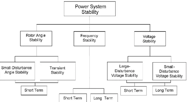
There are two different classifications for voltage stability as shown in Figure 2.1.
Figure 2.1 Classification of power system stability (IEEE/CIGRE, 2004).
Large-disturbance voltage stability refers to the system’s ability to maintain steady voltages following large disturbances such as system faults, loss of generation, or circuit contingencies. This ability is determined by the system and load characteristics, and the interactions of both continuous and discrete controls and protections. Determination of large-disturbance voltage stability requires the examination of the nonlinear response of the power system over a period of time sufficient to capture the performance and interactions of such devices as motors, underload transformer tap changers, and generator field-current limiters. The study period of interest may extend from a few seconds to tens of minutes.
Small-disturbance voltage stability refers to the system’s ability to maintain steady voltages when subjected to small perturbations such as incremental changes in system load. This form of stability is influenced by the characteristics of loads, continuous controls, and discrete controls at a given instant of time. This concept is
useful in determining, at any instant, how the system voltages will respond to small system changes. With appropriate assumptions, system equations can be linearized for analysis thereby allowing computation of valuable sensitivity information useful in identifying factors influencing stability.
As noted above, the time frame of interest for voltage stability problems may vary from a few seconds to tens of minutes. Therefore, voltage stability may be either a short-term or a long-term phenomenon as identified in Figure 2.1.
Long-Term Voltage Instability involves slower acting equipment such as tap-changing transformers, thermostatically controlled loads, and generator current limiters. The study period of interest may extend to several or many minutes, and long-term simulations are required for analysis of system dynamic performance. Instability is due to the loss of long-term equilibrium (e.g., when loads try to restore their power beyond the capability of the transmission network and connected generation), post-disturbance steady-state operating point being small-disturbance unstable, or a lack of attraction toward the stable post-disturbance equilibrium (e.g., when a remedial action is applied too late).
Short-term voltage stability involves dynamics of fast acting load components such as induction motors, electronically controlled loads, and HVDC converters. The study period of interest is in the order of several seconds, and analysis requires solution of appropriate system differential equations. Dynamic modeling of loads is often essential. Short circuits near loads are important.
2.1.2 Definition and classification of voltage stability by EPRI
Definition and Classification of Voltage Stability by EPRI (EPRI, 2009) is made as follows:
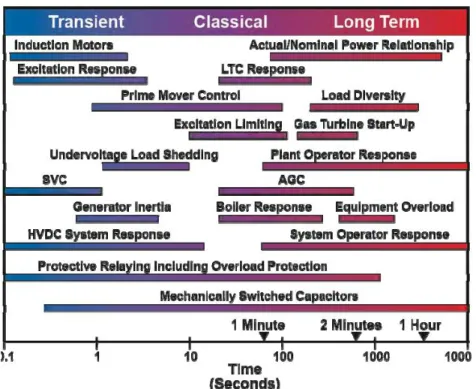
The EPRI Power System Dynamics Tutorial classifies the voltage stability in a different way. Figure 2.2 is provided to relate the time frames for the three different types of voltage instability. Note that different characteristics of the system are involved with each type of instability. For example, to understand transient voltage instability it is necessary to understand how induction motors behave.
Figure 2.2 Time frames for voltage instability (EPRI, 2009).
Short-term or transient voltage instability typically involves large numbers of induction motors stalling and attempting to restart. The motor stalling leads to a large increase in reactive power (Mvar) consumption. If a severe enough shortage of reactive power develops voltage instability may occur.
Table 2.1 Voltage instability types & time frames (EPRI, 2009).
With respect to EPRI and IEEE/CIGRE, transient voltage instability occurs over a short time period. From the initial disturbance to voltage instability time period
typically takes less than 15 seconds. In this study, the results of disturbances for a 10 seconds time period will be considered.
2.2 Example of Transient Voltage Instability in The Literature
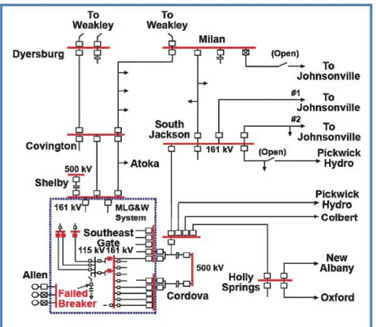
An example of transient voltage instability is given by EPRI (EPRI, 2009). Transient voltage instability is due to the stalling of induction motors took place in and around the Memphis Light Gas & Water (MLG&W) power system August 22, 1987. MLG&W is a large municipal power system which was supplied by the Tennessee Valley Authority (TVA). TVA is a large federal power agency that covers a five state area. Figure 2.3 is a one-line diagram of the MLG&W system and the surrounding TVA system.
Figure 2.3 TVA and MLG&W power systems (red filled boxes shows tripped breakers) (EPRI, 2009).
At 01.20 Saturday morning, August 22, 1987, an air-blast circuit breaker at Southeast Gate substation failed while performing an automatic (voltage controlled) capacitor switching operation.
To clear the damaged breaker at 13.02 the operator began to crank open the disconnects and all three blades maintained arcs when fully opened. The arcs rapidly formed Φ-Φ faults and eventually Φ-ground faults.
There was no differential relaying on the Southeast Gate 115 kV bus. The fault lasted for 78 cycles until it was finally cleared by various backup relays opened the circuit breakers as shown red filled boxes in Figure 2.3. Bus voltages in the area depressed to as low as 60% of normal during the fault. After the fault was cleared area voltages recovered to about 75% of normal.
The initial low voltage and the subsequent recovery to only 75% of nominal caused many area motors to trip or stall. The tripping of area motors was beneficial since this reduced the connected load. However, many motors simply stalled, and as they attempted to regain speed drew huge amounts of Mvar from the system. As was mentioned earlier, this in-rush current may be 5 to 8 times the normal load current requirements of the motors.
Much of the motor load consisted of 1Φ air-conditioner compressors. These motors often do not have any type of undervoltage protection to trip off-line. During the disturbance, which lasted 10 to 15 seconds, large portions of compressor motor load stalled and tried to regain speed. As the Memphis area reactive demands increased the surrounding TVA system was called upon to supply the additional reactive power.
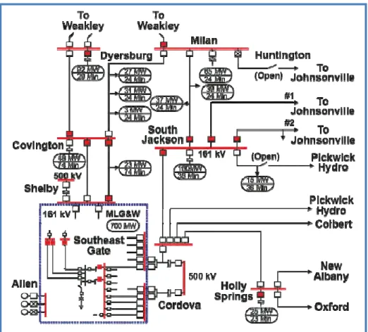
The most severe impact was 70 miles to the north in the Covington, Jackson, and Milan areas where reactive power is supplied primarily by shunt capacitor banks. The prevailing low voltage resulted in low shunt capacitor reactive output. In addition, several key area lines and generators were out for maintenance. The two 161 kV lines from Johnsonville to South Jackson were heavily loaded with MW and Mvar power. Within two seconds of the initial disturbance both of these lines tripped due to operation of reverse zone 3 distance relays. After the loss of these two lines voltage at South Jackson fell to 67% of normal.
Over the next 5 seconds, the rest of the 161 kV lines into Covington, Milan, and South Jackson tripped due to the low voltage and the high current flows. TVA lost a total of 565 MW of load while MLG&W lost 700 MW of load. Figure 2.4 illustrates
the breakers that tripped as red filled boxes. The oval boxes state the MW lost and the time it took to restore the load.
Figure 2.4 Post disturbance system conditions (red filled boxes shows tripped breakers) (EPRI, 2009).
2.3 Literature Survey
The basic concepts and definitions of voltage stability issue is given in detail (EPRI, 2009) and (Kundur, 1994).
Static and Dynamic voltage stability analysis is studied, short-term and long-term voltage stability is investigated in (Pothula, 2010). There is also a proposed methodology to determine voltage stability index.
The critical role played by induction motors in short-term voltage stability phenomenon, and emphasizes the need for including proper dynamic models of motor loads in voltage stability related planning studies is presented in (Krishnan, 2012).
Using P-V curves and Q-V curves to study voltage instability is expressed in (Bhaladhare et al., 2013). It is observed from study that real power transfer increases from lagging to leading power factor. Using the Q-V curves the sensitivity of the load to the reactive power sources can be obtained. Thus basic voltage stability analysis tools i.e. P-V curve and Q-V curve are found to be effective tools to understand static voltage stability analysis.
The problems encountered in system voltages for a fast growing utility of the Sultanate of Oman are discussed by Khan (1999). The power system encountered voltage stability problems during peak summer conditions. The voltage collapse is induced by shortfall in Mvar supplied. This problem has been investigated by the use of PV and QV curves methods. The computations for voltage stability were carried out by modeling all loads in the system as constant power. The loads and generating units are lumped. Steady-state analysis carried out and system wide weak buses have been identified.
Critical period for voltage problems during summer days and its effect on remote load buses in terms of voltage profile is discussed and recommendations proposed to remedy the voltage problems. Immediate remedial action is installation of recommended Q-support (voltage controlled capacitors) at weak buses in the system (33 kV level). Future actions which were recommended, will ‘completely eradicate’ future voltage problems in the system. These include comprehensive load modeling, modal analysis of the system, monitoring of 11 kV loads, SVC implementation, load shedding and additional generation, etc. (Khan, 1999).
Dynamic voltage stability analysis requires the modeling of real power system and make simulations. The power system components like governors, turbines and exciters of synchronous generators are represented as functional block diagrams for dynamic analysis of power system. These are approximate nonlinear mathematical models. The IEEE Task Force on Overall Plant Response considered the effects of power plants on power system stability and issued a report about dynamic modeling (IEEE Committee Report, 1973).
The Hsin-Chu Science-Based Industrial Park established in 1980 is one of the most important high-tech semiconductor industries in Taiwan. The needs of power service quality and reliability of industrial park is much higher than those of general
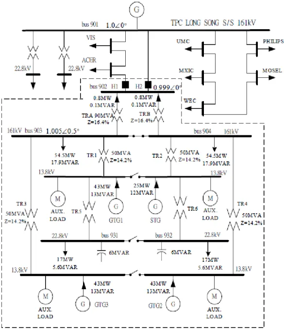
customers. The power service outage due to Taiwan Power Company (Taipower) system fault causes serious production loss for the high-tech customers. In Hsin-Chu Science-Based Industrial Park there is an industrial cogeneration system “Hsin-Yu Cogeneration Plant” that consists of one steam turbine and three gas turbines as shown in Figure 2.5.
Figure 2.5 One-line diagram of the cogeneration system (Hsu, 2007).
Improvement of voltage sags in Hsin-Chu Science-Based Industrial Park by installation of the Hsin-Yu Cogeneration Plant is presented by Hsu (2007). The cogeneration system is installed to mitigate the voltage sags due to external system
faults. A voltage sag ride-through curve has been adopted in this paper to evaluate the effect of voltage sags (Hsu, 2007).
The under voltage relays to disconnect the cogeneration system from the utility are designed by considering the critical clearing times at the point of common coupling and voltage sags ride-through curves. The dynamic responses of different fault conditions are executed by using the transient stability analysis to calculate and define the voltage sags ride-through curves with and without considering the disconnection of the cogeneration system. It is concluded that the voltage sags ride-through capability can be improved greatly if the cogeneration systems are performed to trip accurately according to the under voltage relays design proposed (Hsu, 2007).
A transient frequency stability study of Hsin-Yu Cogeneration Plant for different operation modes is carried out by the use of ETAP software (Chen et al., 2010). The mathematical models are established for generators, exciters, governors, loads and other equipment. Aim of the study is to examine the frequency behavior of the plant in case of decoupling from Grid after a tie line tripping, with or without load shedding.
Frequency load shedding scheme is studied in conjunction with decoupling logic for different operation mode. The simulations show that there is a close coherence between pre-fault load conditions, pre-fault power generation, decoupling scheme, settings of the load shedding and frequency behavior in the plant (Chen et al., 2010).
A transient stability study of the Hsin Yu Co-Generation plant in Hsin-Chu Science Based Industrial Park for different operation modes was carried out (Zimmerman et al., 2000). The network calculation program CALPOS by ABB is used for modeling and analysis in this study. Aim of the study was to examine the behavior of the plant in case of internal and external faults. The determined critical clearing times provides general information about the influence of pre-fault load conditions, pre-fault power generation and fault location on the transient stability of the generators.
The critical clearing time calculations are used to find the settings of the de-coupling scheme for the voltage relay and the frequency relay. A load shedding
scheme was studied in conjunction with the de-coupling logic. The simulations show that there is a close coherence between the de-coupling scheme, the settings of the load shedding stages and the frequency behavior in the plant (Zimmerman et al., 2000).
Short-term voltage stability enhancement by using the Static Synchronous Compensator (STATCOM) is discussed in (Dong et al., 2014). A practical approach is presented for dynamic load modeling of industrial feeders and placing Static Synchronous Compensator (STATCOM) devices for dynamic VAR support to enhance the short-term voltage stability.
The key subjects defining and classifying voltage stability is given in detail in literature. The primary power system components that have effect on voltage stability and analysis methods are discussed in several studies. The static and dynamic voltage stability analysis has been done in different studies and enhancement of voltage stability is also discussed.
This thesis have similarities with some studies in that the effect of decoupling time and load shedding after decoupling on transient voltage stability have been analyzed for an industrial power plant. The exception from other studies is that, for some certain situations it is demonstrated by the analysis that transient voltage stability is enhanced by only electrical network configuration change.
2.4 Voltage Stability Analysis Methods
Voltage stability analysis can be done by static and dynamic methods. In static analysis snapshots of system conditions at a time instant is used. In dynamic analysis the power system dynamic model is used to make time domain simulations. Dynamic analysis gives more accurate results for voltage instability and this is useful for detailed study of a specific system.
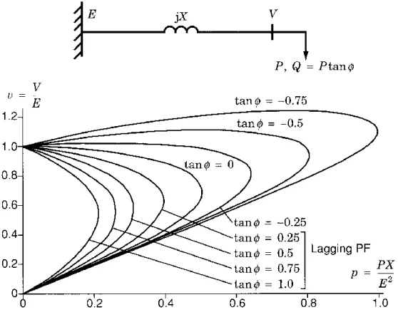
PV and QV curves are used to determine voltage stability limits or margins for slow voltage decay. Static loads are used in this method. PV Curves obtained by power flow solution with a software that provide the voltage magnitude and angle at each bus, and the real and reactive power flows on the lines. When the real power flow increases the voltage magnitudes tend to decrease. There is point shows
instability on the PV curves at the tip or the “nose” that the system can no longer support the real power flow on the lines and maintain a stable voltage, thus voltage collapses. PV curves for different power factors is shown in Figure 2.6.
Figure 2.6 Normalized P-V Curves. (Taylor, 1994)
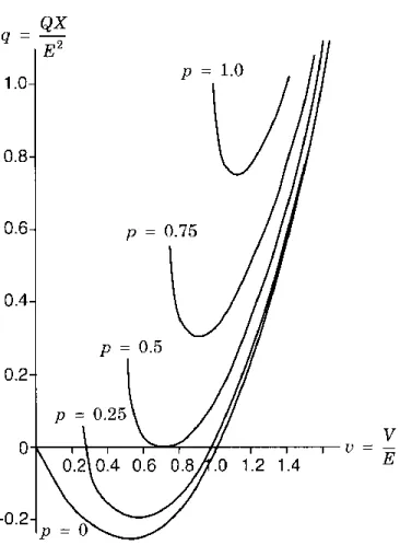
The QV curve relates the voltage on a bus to the reactive power available at that bus. As voltage increases on a bus, more reactive power flows from that bus to the rest of the system. The analysis of QV curves is based on an unlimited fictitious reactive power source that controls the voltage at the QV test bus by either supplying or absorbing reactive power to force the voltage up or down at that bus. Figure 2.7 shows an example of a set of QV curves for a system at different load levels. The “p=” in the graphs represents the fixed normalized real power of the loads. The instability point of the QV curve is at the bottom of the curve. This is when the reactive power on the bus no longer increases as the voltage decreases. The reactive power margin is negative if the curve does not pass below the 0 Mvar axis (Johnson, 2011).
Figure 2.7 Normalized Q-V Curves (Taylor, 1994).
Transient (short-term) voltage stability that simulated with detailed motor loading data, involves dynamics of fast acting system components. Voltage recovery or collapse for post contingency is studied. Study period of interest is in the order of a seconds and in this study we will analyze 10 second time interval. Dynamic model is used for loads and analysis requires solution of differential equations using time-domain simulations. To show the voltage collapse or recovery the voltage magnitude at each bus is plotted against time. Because the voltage is directly affected, faults/short-circuits near loads could be important.
CHAPTER 3
MODELING OF POWER SYSTEM ELEMENTS 3.1 Load Model Category
The analysis is made on system models. The load models are divided into two categories: static and dynamic. A composite load model includes both static and dynamic elements to represent the aggregate characteristics of some loads.
3.1.1 Static load model
The static model of the load provides the active and reactive power needed at any time based on simultaneously applied voltage and frequency. Static load models are capable of representing static load components such as resistive and reactive elements. They can also be used as a low frequency approximation of dynamic loads such as induction motors. However the static load model is not able to represent the transient response of dynamic loads (IEEE, 1993).
Traditionally there are three types of static load models: voltage dependent, constant impedance/current/power (ZIP), and frequency dependent. The active and reactive power component of static load model are always treated separately (IEEE, 1993; Kundur, 1994).
3.1.2 Dynamic load model
A dynamic load model is a differential equation that gives the active and reactive power at any time based on instantaneous and past applied voltage and frequency (IEEE, 1993). Dynamic model parameters are used for modeling of induction motor loads in analysis software. Typical devices and controls that contribute to load dynamics are:
Induction motor
Protection system
Discharge lamp
Other devices with dynamics such as HVDC converter, transformer ULTC, voltage regulator, and so on
Modeling dynamic load is much more difficult than modeling static load but is essential for short term voltage stability studies.
3.1.3 Composite load model
To represent aggregate characteristics of various load components, it is necessary to consider composite load models that take into account both static and dynamic behavior (IEEE, 1993; Kundur, 1994). Models of the following components are generally needed in a composite model:
Large industrial, commercial type or small appliance induction motors
Discharging lights
Heating and incandescent lighting load
Thermostatically controlled loads
Power electronic loads
Transformer saturation effects
Shunt capacitors
The composite load model also includes different representation for;
The percentage of each type of load components
Parameter differences of similar load component types
The parameters of the feeders such as impedance and admittance.
Each power operation management groups may have their own special composite load model for power system analysis. The composite model could also change with the different requirements. For example, the composite load model used by WECC in 2006 includes 20% induction motor load (dynamic), 80 % static load. Recently WECC has proposed a new composite load model that includes transformers, shunt capacitors, feeder equivalent, three-phase induction motors, and equivalent models for air conditioners (Kosterev, 2006).
3.1.4 Voltage instability & induction motor stalling
When an induction motor is first started (or has stalled and is rebuilding speed) it may draw 5 to 8 times its normal Mvar to build its magnetic field. This in-rush of reactive power typically lasts only a few seconds but can severely depress system voltages. The amount of Mvar an induction motor draws from the power system is directly related to its speed (EPRI, 2009).
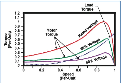
Torque/Speed Curves illustrate the relationship between motor speed and the available accelerating torque as in Figure 3.1. The four curves in Figure 3.1, labeled rated voltage, 80% voltage and 60% voltage, represent the available torque to accelerate the motor at three different system voltage levels and fourth curve labeled load torque represent the load torque of the load. The induction motor accelerates to near rated speed as long as the system voltage is greater than 80% of nominal. If the motor is running at less than 45% of rated speed and the system voltage is 60% of nominal, the motor never reaches its rated speed. The motor draws large amounts of reactive current until hopefully its thermal protection trips it off line.
Figure 3.1 Induction motor torque/speed curve (EPRI, 2009).
After a severe voltage disturbance strikes a system with a heavy concentration of induction motors, voltage declines which causes the induction motors to slow down. Once the system voltage starts to recover the motor load automatically tries to
pick up speed. The in-rush of Mvar to return the motors to rated speed may be enough to trigger transient voltage instability.
The declining voltages due to the sudden increase in Mvar demand may cause uncontrolled tripping and the rapid collapse of the area power system. This sequence of events is classified as short-term or transient voltage instability due to the speed of the events. The entire process typically last less than 15 seconds.
3.2 Load Torque Characteristic
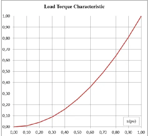
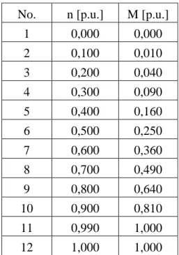
The characteristic curve for load torque must be available for the motor’s entire speed range. The load torque is treated separately from the network's electrical characteristics and attributes. The load torque must always be smaller than motor torque for the motor to attain proper speed. A Load/torque curve used in modeling of the loads is given in Figure 3.2 and the related values are in Table 3.1.
No. n [p.u.] M [p.u.] 1 0,000 0,000 2 0,100 0,010 3 0,200 0,040 4 0,300 0,090 5 0,400 0,160 6 0,500 0,250 7 0,600 0,360 8 0,700 0,490 9 0,800 0,640 10 0,900 0,810 11 0,990 1,000 12 1,000 1,000
Table 3.1 Torque/speed values of a typical load.
3.3 Governor Model
Synchronous generators are main source of electricity in power systems. Active and reactive power produced by the generators directly effects the voltage stability. The governors, turbines and exciters of synchronous generators are represented as functional block diagrams in models for dynamic analysis of power system. These are approximate nonlinear mathematical models.
Generators use governor control systems to control the shaft’s speed of rotation and active power generated at terminals. The governor system senses generator shaft speed deviations and initiates adjustments to the mechanical input power of the generator to increase or decrease the generator’s speed as required. IEEE Type 1 Turbine-Governor Model IEEEG1 (Siemens, 2012) is used for the modeling of governor and turbine and it includes function blocks. The model is shown in Figure 3.3, the used parameter values are below in Table 3.2.
Figure 3.3 Turbine-governor model IEEEG1 (Siemens, 2012).
Stages of Steam Turbine 4 – Reheater
5 – Crossover 6 - Double Reheat
Speed Governor K=1/R
Servomotors and Governor Controlled Valves
Description Def. Min Max Actual
JBUS 0 0
M 0 0
K Governor gain (1/droop) 20 5 30 20
T1 (sec) Governor lag time constant 0,5 0 4,99 0,1
T2 (sec) Governor lead time constant 1 0 9,99 0
T3 (>0) (sec) Valve positioner time constant 1 0,041 1 0,1
Uo (pu/sec) Maximum valve opening velocity 0,1 0,01 0,3 0,18
Uc (<0) (pu/sec) Maximum valve closing velocity -0,2 -0,3 -0,01 -0,18
PMAX (pu) Maximum valve opening 1 0,5 2 1
PMIN (pu) Minimum valve opening 0 0 0,49 0,02
T4 (sec) Inlet piping/steam bowl time const 0,4 0,01 1 0,3
K1 Fraction of hp shaft power after first boiler pass
0,2 -2,0 1 0,994
K2 Fraction of lp shaft power after first boiler pass
0 0 0 0
T5 (sec) Time constant of second boiler pass 7 0 9,99 0,001
K3 Fraction of hp shaft power after second boiler pass
0,1 0 0,49 0,001
K4 Fraction of lp shaft power after second boiler pass
0 0 0,49 0,001
T6 (sec) Time constant of third boiler pass 0,6 0 9,99 0,001
K5 Fraction of hp shaft power after third boiler pass
0,2 0 0,34 0,001
K6 Fraction of lp shaft power after third boiler pass
0 0 0,54 0,001
T7 (sec) Time constant of fourth boiler pass 0,3 0 9,99 0,001
K7 Fraction of hp shaft power after fourth boiler pass
0,1 0 0,29 0,001
K8 Fraction of lp shaft power after fourth boiler pass
0 0 0,29 0,001
3.4 Exciter Model
The excitation systems of the generators have control, limiting and protection functions. The output voltage, power factor (cosØ) and reactive power produced at generator terminals is controlled by the exciter by controlling the field current. This enhance the voltage stability of power system.
IEEE Type 2 Excitation System Model IEEEX2 (Siemens, 2012) is used for the modeling of exciters. The model is shown in Figure 3.4, the used parameter values are below in Table 3.3.
Figure 3.4 Excitation system model IEEEX2 (Siemens, 2012).
1 - EField :Field voltage of the exciter output 2 - Sensed Vt : Measured voltage value 3 – LL : Regulator output
4 – VR : Amplifier output of regulated signal 5/6 – VF1/VF2 : Damping signals
Description Default Min Max Used Value TR (sec) 0,02 0 0,49 0,03 KA 80 10,01 499,99 44,2 TA (sec) 0,1 0 0,99 0,01 TB (sec) 0,1 0 0,06 TC (sec) 1 0 0,34 VRMAX or zero 5 0,51 9,99 8,83 VRMIN -5 -9,99 -0,01 -8,83 KE or zero 0,7 -1 1 0 TE (> 0) (sec) 0,1 0,041 0,99 0,34 KF 0,03 0 0,29 0,04 TF1 (> 0) (sec) 0,11 0,041 1,49 1,0 TF2 (> 0) (sec) 1 0,041 1,49 1,0 E1 4 0 3,8 SE (E1) 0,4 0 0,99 0,716 E2 5 0 5,07 SE (E2) 0,5 0 0,741
CHAPTER 4 SIMULATION 4.1 Simulation Software
PSS (Power Systems Simulator) SINCAL (Siemens Network Calculator) Software by SIEMENS is used for the analysis and simulation in this project (Siemens, 2013).
SINCAL is a software package with planning tools for electricity. Functions relevant to power systems analysis include load flow (balanced and unbalanced), short circuit, time-domain dynamic simulations, eigenvalue and modal analysis, harmonic analysis, protection simulations, reliability and contingency analysis.
PSS®SINCAL Stability calculations analyze the behavior of electrical networks when there are malfunctions or disturbances. A power system is stable, if it returns to a steady-state or equilibrium operating condition following a disturbance.
To assure network stability, the following criteria need to be checked in detail:
Voltage stability
Rotor angle stability
Transient stability
Rotor angle swing
PSS®SINCAL’s calculation module for stability has been developed precisely to check these criteria. This calculation module is based on the PSS®NETOMAC program package, one of programs for observing all kinds of dynamic procedures in electrical networks.
In stability calculations, the network is only simulated with complex impedances. Controllers and machines are, however, modeled as differential equations. The examined system is simulated symmetrically.
In order to consider unsymmetrical faults in addition to symmetrical faults such as three-phase short circuits, PSS®SINCAL uses symmetrical components (positive-,
zero- and negative-phase sequence) to create a universal disturbance scenario. The faults in the network and the associating switching can be modeled in detail.
This calculation module is used for investigations for which the envelope curves of the characteristic values are sufficient results. The modeling for networks and machines being investigated can be as complex as you want, i.e. even networks with thousands of nodes and hundreds of machines can be investigated without any problem. So you can recreate controller behavior for equipment,
PSS®SINCAL provides controller database containing the various predefined controllers:
IEEE standards
Excitation systems
Turbine governors
Power System Stabilizer (PSS)
PSS®E controller models
Generic wind models
4.2 Modeling of Industrial Cogeneration System
Like refinery, petrochemical, steel and many other important industrial power systems should be reliable. A typical single line diagram and the issues related to power system reliability is given by Khan (2008). Also the general structure of a typical power system for Oil and Gas industry is explained by Devold (2013).
By use of the above references and from industrial experience a typical industrial power plant is modeled for simulation and analysis in SINCAL software as shown in Figure 4.1. This plant is assumed as an industrial cogeneration system including electrical distribution system to the factories of an industrial zone.
The power system is connected to the GRID by two overhead lines at 154 kV level. The distribution to the factories is at 34,5 kV voltage level. There are two buses at 154 kV level, two buses at 34,5 kV level and two step-down transformers with OLTC between 154 kV & 34,5 kV buses.
Power plant has one Gas Turbine (GT) connected to 154 kV bus, and two Steam Turbines (ST) connected to the 34,5 kV bus. Each turbine has 40 MW capacity, total power plant production capacity is 120 MW. Total load of industrial zone is 75 MW. Depending on the operation conditions of both power plant and factories, power export as well as power import is possible.
The GT has an HRSG to produce steam from the exhaust gas. Also there is two conventional boilers to produce steam for factories and STs. The steam system, Boilers and HRSG of GT are not modeled in this study.
There are six factories in industrial zone and each factory is fed by two cable feeders. Each feeder has its own step-down transformer (34,5 kV / 6,3 kV) feeding each 6,3 kV factory bus. The factory loads are at 6,3 kV level and represented as lump sum of related smaller loads. The majority of loads are motor loads.
At each voltage level there is bus coupler between buses. In normal operation 154 kV and 34,5 kV bus couplers are closed, factory 6,3 kV bus couplers are open. 4.3 Criteria for Transient Voltage Stability
Several conditions are simulated and some specific bus voltages analyzed. There should be some criteria to identify the existence of transient voltage stability.
The protection relay of induction motor or other equipment may be actuated when the bus voltage drops a certain level and doesn’t recover for a certain time (example: 0.8 pu and 0,8 second) and resulting high load current. For a stable system there should not any equipment tripping.
Following table describes WECC Disturbance-Performance Table of Allowable Effects on Other Systems (WECC, 2007).
NERC and WECC Category Outage Frequency Associated with Performance Cat. (outage/year) Transient Voltage Dip Standard Minimum Transient Frequency Standard Post Transient Voltage Deviation Standard B 0,33 Not to exceed 25% at load buses or 30% at nonload buses. Not to exceed 20% for more than 20 cycles at load buses. Not below 59.6 Hz for 6 cycles or more at a load bus. Not to exceed 5% at any bus. C 0,033-0,33 Not to exceed 30% at any bus. Not to exceed 20% for more than 40 cycles at load buses. Not below 59.0 Hz for 6 cycles or more at a load bus. Not to exceed 10% at any bus.
Table 4.1 WECC Disturbance-Performance Table (WECC, 2007).
In this study Category C disturbance criteria (WECC, 2007) is used to determine the transient voltage stability for the concerned buses. Transient Voltage Dip not to exceed 20% of nominal voltage for more than 40 cycles (800 ms) at load buses and Post Transient Voltage Deviation not to exceed 10% of nominal voltage at any bus.
CHAPTER 5 CASE STUDIES 5.1 Overview
The behavior of power system for external fault is examined in this thesis. It is assumed that fault point is nearest GRID 154 kV bus that is infinite bus and there is 3 phase short circuit fault that is most severe fault in power systems. Power system network configuration is shown in Figure 5.1.
Several cases are simulated with different parameters and resulting effects on transient voltage stability investigated. Cases will show the stable and unstable situations of power system for transient voltage stability. The studied cases are obtained by changing some specific system parameters or network configuration.
According to the fault type, fault location, situation of generators and loads, shedding of predetermined loads according to their importance, circuit breaker positions, protection relay time delays etc. many different cases may be obtained for simulation. In this thesis three of them are selected and studied:
Case-1: Decoupling time
Case-2: Load shedding after decoupling (L1&L2 feeders of Plant-1/2/4)
Case-3: Power system network configuration
To accept the power system is stable for any of these cases, the transient voltage stability criteria should satisfied for all selected buses; 154 kV Bus-1, 34,5 kV Bus-B, Plant-5 6,3 kV Bus-1 which are shown in Figure 4.1 as red colored buses. The transient voltage stability criteria is; The voltage is recovered above 0,8 pu voltage level within TDrf < 800 ms (recovery duration from fault beginning) time.
Simulations are based on some assumptions:
System is balanced, load and generation is close to each other.
There is a 3 phase short circuit at the nearest GRID 154 kV bus.
Decoupling of power plant from GRID will be with a time delay TDd.
Figure 5.1 Industrial cogeneration system network configuration (154 kV & 34,5 kV).
5.2 Simulation of Cases
5.2.1 Case-1: Decoupling time
Effect of decoupling time duration “TDd” on the transient voltage stability can be simply shown by two different time values. These TDd time values include delay time of relay and operation time of relay and circuit breaker.
According to the Electricity Market Grid Regulation (TEİAŞ, 2003) maximum fault clearance time for 154 kV overhead lines is 140 ms. First simulation is made with TDd = 200 ms decoupling time duration (long relay time delay). This TDd time is chosen so that fault may be cleared by the GRID protection system before
decoupling. The graphs in Figure 5.2 are showing 154 kV - 34,5 kV - 6,3 kV bus voltages for this case.
It can be seen from graphs in Figure 5.2 that TDrf value (recovery duration from fault beginning) is very high for all three buses and transient voltage stability is not satisfied.
It was assumed that the minimum TDd time is 70 ms with zero delay time of relay. By using a short delay time of relay as 30 ms, second simulation is made with TDd = 100 ms. The graphs in Figure 5.3 are showing 154 kV - 34,5 kV - 6,3 kV bus voltages for this case. It can be seen from graphs in Figure 5.3 that TDrf value is 340 ms for 6,3 kV bus, 320 ms for 34,5 kV bus and 300 ms for 154 kV bus. Transient voltage stability is satisfied for all three buses.
As can be seen from results in Figure 5.3 TDrf value is higher for 6,3 kV bus when compared to 34,5 & 154 kV buses and so it is more sensitive for stability.
Case-1 Simulation graphs for TDd = 200 ms 0 0,1 0,2 0,3 0,4 0,5 0,6 0,7 0,8 0,9 1 1,1 0 0,2 0,4 0,6 0,8 1 1,2 1,4 1,6 1,8 2 2,2 2,4 2,6 2,8 3 3,2 3,4 3,6 3,8 4 [pu] t [s]
PLANT 154KV BUS-1 VOLTAGE
Tf Td Tr (a) 0 0,1 0,2 0,3 0,4 0,5 0,6 0,7 0,8 0,9 1 1,1 0 0,2 0,4 0,6 0,8 1 1,2 1,4 1,6 1,8 2 2,2 2,4 2,6 2,8 3 3,2 3,4 3,6 3,8 4 [pu] t [s] 34.5KV BUS-B VOLTAGE Tf Td (b) 0 0,1 0,2 0,3 0,4 0,5 0,6 0,7 0,8 0,9 1 1,1 0 0,2 0,4 0,6 0,8 1 1,2 1,4 1,6 1,8 2 2,2 2,4 2,6 2,8 3 3,2 3,4 3,6 3,8 4 [pu] t [s]
PLANT-5 6.3KV BUS-1 VOLTAGE
Tf Td
(c)
Figure 5.2 Case-1 simulation graphs for TDd = 200 ms a) 154 kV bus voltage, b) 34,5 kV bus voltage, c) 6,3 kV bus voltage.
Case-1 Simulation graphs for TDd = 100 ms 0 0,1 0,2 0,3 0,4 0,5 0,6 0,7 0,8 0,9 1 1,1 0 0,2 0,4 0,6 0,8 1 1,2 1,4 1,6 1,8 2 2,2 2,4 2,6 2,8 3 3,2 3,4 3,6 3,8 4 [pu] t [s]
PLANT 154KV BUS-1 VOLTAGE
Tf Td Tr (a) 0 0,1 0,2 0,3 0,4 0,5 0,6 0,7 0,8 0,9 1 1,1 0 0,2 0,4 0,6 0,8 1 1,2 1,4 1,6 1,8 2 2,2 2,4 2,6 2,8 3 3,2 3,4 3,6 3,8 4 [pu] t [s] 34.5KV BUS-B VOLTAGE Tf Td Tr (b) 0 0,1 0,2 0,3 0,4 0,5 0,6 0,7 0,8 0,9 1 1,1 0 0,2 0,4 0,6 0,8 1 1,2 1,4 1,6 1,8 2 2,2 2,4 2,6 2,8 3 3,2 3,4 3,6 3,8 4 [pu] t [s]
PLANT-5 6.3KV BUS-1 VOLTAGE
Tf Td
Tr
(c)
Figure 5.3 Case-1 simulation graphs for TDd = 100 ms a) 154 kV bus voltage, b) 34,5 kV bus voltage, c) 6,3 kV bus voltage.
To find critical decoupling time duration value, TDd value is increased with small steps starting from 100 ms. TDd = 125 ms value is achieved when the TDrf ~ 800 ms is obtained for 6,3 kV bus. Simulation results of this value for three buses shown in Figure 5.4.
The resulting TDd = 125 ms value can be accepted as critical decoupling time duration value for transient voltage stability of power system.
Case-1 Simulation graphs for TDd = 125 ms 0 0,1 0,2 0,3 0,4 0,5 0,6 0,7 0,8 0,9 1 1,1 0 0,2 0,4 0,6 0,8 1 1,2 1,4 1,6 1,8 2 2,2 2,4 2,6 2,8 3 3,2 3,4 3,6 3,8 4 [pu] t [s]
PLANT 154KV BUS-1 VOLTAGE
Tf Td Tr (a) 0 0,1 0,2 0,3 0,4 0,5 0,6 0,7 0,8 0,9 1 1,1 0 0,2 0,4 0,6 0,8 1 1,2 1,4 1,6 1,8 2 2,2 2,4 2,6 2,8 3 3,2 3,4 3,6 3,8 4 [pu] t [s] 34.5KV BUS-B VOLTAGE Tf Td Tr (b) 0 0,1 0,2 0,3 0,4 0,5 0,6 0,7 0,8 0,9 1 1,1 0 0,2 0,4 0,6 0,8 1 1,2 1,4 1,6 1,8 2 2,2 2,4 2,6 2,8 3 3,2 3,4 3,6 3,8 4 [pu] t [s]
PLANT-5 6.3KV BUS-1 VOLTAGE
Tf Td
Tr
(c)
Figure 5.4 Case-1 simulation graphs for TDd = 125 ms a) 154 kV bus voltage, b) 34,5 kV bus voltage, c) 6,3 kV bus voltage.
5.2.2 Case-2: Load shedding after decoupling
The simulations of Case-1 showed that the power system is not stable for decoupling time duration TDd = 200 ms (long relay time delay).
There may be a necessity to use TDd = 200 ms decoupling time duration for waiting the fault is cleared by the GRID protection system. But in this case the power system and factories will shut-down because of transient voltage instability as shown in Figure 5.2. One possible solution for this problem is to make load shedding.
Load shedding will reduce active and reactive power demand and reduce stress on the power system. This makes easy to voltage recovery and may prevent shut-down. For this purpose some loads should be preselected to shed.
To illustrate this case some motor feeders are chosen and assumed as less critical with respect to others as shown in Figure 5.5: 1_L1, 2_L1, Plant-4_L1, Plant-1_L2, Plant-2_L2, Plant-4_L2. The Total load to be shed; active power is 27,5 MW and reactive power is 15,5 Mvar.
Protection relays of these motor feeders are used for shedding of them. Low voltage protection function with time delay can be used for this purpose.
Ideally the low voltage setting of protection relay should be lower than the critical voltage level for stability that is <U ≤ 0,8 pu. From Case-1 simulation graphs for TDd = 200 ms in Figure 5.2 (c) the voltage of 6,3 kV bus drops and not exceed 0,7 pu value for a long time. So the low voltage setting of relay can be chosen as <U = 0,7 pu.
For low voltage protection, delay time of relay should be at least TDlv = 200 ms to be sure that power system have passed to the island operation. By assuming relay and circuit breaker total operation time as 70 ms, the loads will be shed 270 ms after beginning of fault. Simulation results of this case is shown in Figure 5.6.
It can be seen from graphs in Figure 5.6 that TDrf value is 750 ms for 6,3 kV bus, 490 ms for 34,5 kV bus and 480 ms for 154 kV bus. Transient voltage stability is satisfied for all three buses.
Case-2 Simulation graphs for TDd = 200 ms & TDlv = 200 ms 0 0,1 0,2 0,3 0,4 0,5 0,6 0,7 0,8 0,9 1 1,1 0 0,2 0,4 0,6 0,8 1 1,2 1,4 1,6 1,8 2 2,2 2,4 2,6 2,8 3 3,2 3,4 3,6 3,8 4 [pu] t [s]
PLANT 154KV BUS-1 VOLTAGE
Tf Td Tr (a) 0 0,1 0,2 0,3 0,4 0,5 0,6 0,7 0,8 0,9 1 1,1 0 0,2 0,4 0,6 0,8 1 1,2 1,4 1,6 1,8 2 2,2 2,4 2,6 2,8 3 3,2 3,4 3,6 3,8 4 [pu] t [s] 34.5KV BUS-B VOLTAGE Tf Td Tr (b) 0 0,1 0,2 0,3 0,4 0,5 0,6 0,7 0,8 0,9 1 1,1 0 0,2 0,4 0,6 0,8 1 1,2 1,4 1,6 1,8 2 2,2 2,4 2,6 2,8 3 3,2 3,4 3,6 3,8 4 [pu] t [s]
PLANT-5 6.3KV BUS-1 VOLTAGE
Tf Td
Tr
(c)
Figure 5.6 Case-2 Simulation graphs for TDd = 200 ms & TDlv = 200 ms a) 154 kV bus voltage, b) 34,5 kV bus voltage, c) 6,3 kV bus voltage.
LV Load shedding LV Load shedding LV Load shedding
It is seen from previous simulation for TDlv = 200 ms that the transient voltage stability is satisfied for all three buses. To prevent unnecessary load shedding the longer TDlv time can be chosen for low voltage protection relay. But TDrf voltage recovery time duration should be less than 800 ms and so the loads should be shed before 800 ms from beginning of the fault. By assuming relay and circuit breaker
total operation time as 70 ms, maximum TDlv time can be calculated as TDlv = 800 – 70 = 730 ms. Simulation results shown in Figure 5.7.
It can be seen from graphs in Figure 5.7 that TDrf value is 820 ms for 6,3 kV bus, 800 ms for 34,5 kV bus and 800 ms for 154 kV bus. Transient voltage stability is satisfied for 34,5 kV and 154 kV buses, and acceptable for 6,3 kV bus.
Simulation results of this case has shown that for TDd = 200 ms decoupling time duration; transient voltage stability is satisfied for both TDlv values of 200 ms and 730 ms. It can be concluded that decoupling time duration can be increased by load shedding.
Case-2 Simulation graphs for TDd = 200 ms & TDlv = 730 ms 0 0,1 0,2 0,3 0,4 0,5 0,6 0,7 0,8 0,9 1 1,1 0 0,2 0,4 0,6 0,8 1 1,2 1,4 1,6 1,8 2 2,2 2,4 2,6 2,8 3 3,2 3,4 3,6 3,8 4 [pu] t [s]
PLANT 154KV BUS-1 VOLTAGE
Tf Td Tr (a) 0 0,1 0,2 0,3 0,4 0,5 0,6 0,7 0,8 0,9 1 1,1 0 0,2 0,4 0,6 0,8 1 1,2 1,4 1,6 1,8 2 2,2 2,4 2,6 2,8 3 3,2 3,4 3,6 3,8 4 [pu] t [s] 34.5KV BUS-B VOLTAGE Tf Td Tr (b) 0 0,1 0,2 0,3 0,4 0,5 0,6 0,7 0,8 0,9 1 1,1 0 0,2 0,4 0,6 0,8 1 1,2 1,4 1,6 1,8 2 2,2 2,4 2,6 2,8 3 3,2 3,4 3,6 3,8 4 [pu] t [s]
PLANT-5 6.3KV BUS-1 VOLTAGE
Tf Td
Tr
(c)
Figure 5.7 Case-2 Simulation graphs for TDd = 200 ms & TDlv = 730 ms a) 154 kV bus voltage, b) 34,5 kV bus voltage, c) 6,3 kV bus voltage.
LV Load shedding LV Load shedding
5.2.3 Case-3: Power system network configuration
The Modeled power system is flexible and enable different network configurations. This flexibility may be used to enhance stability. The situation that analyzed for this case is stopping ST (steam turbine) UNIT-1 for maintenance. Load shedding will not used in this case.
In Case-1 the simulation graphs for TDd = 100 ms has shown in Figure 5.3 where three generators in service and power system is stable. To show the effect of one generator absence on power system, the same simulation will be repeated with TDd = 100 ms while ST UNIT-1 is stopped, and resulting simulation graphs will be compared with the Figure 5.3.
When ST UNIT-1 is stopped and Case-1 simulation with TDd = 100 ms is repeated, simulation graphs in Figure 5.8 is obtained.
Voltage graph of 6,3 kV bus in Figure 5.3 (c) is compared with Figure 5.8 (c) and it is found that;
Voltage dip value is 0,35 pu, voltage recovery time duration TDrf is 350 ms and system is stable in Figure 5.3 (c).
Voltage dip value is 0,27 pu and voltage is not recovered, power system shut-down in Figure 5.8 (c).
From comparison of two simulations it can be concluded that absence of one generator close to load (on 34,5 kV) is resulting a lover voltage dip value and lack of reactive power source to recover the voltage.
The normal way to overcome this problem is to put a new generator instead of ST UNIT-1 to supply directly the 34,5 kV bus. This new generator will serve to recover the voltage of load buses 34,5 kV & 6,3 kV. This solution requires investment and creates new costs.
The purpose of this study is to solve the problems by operational way if possible and provide transient voltage stability.