Taguchi Techniques for 2k Fractional Factorial Experiments

Volume 34 (2005), 83 – 93

TAGUCHI TECHNIQUES

FOR 2

k

_{FRACTIONAL FACTORIAL}

EXPERIMENTS

Nazan Danacıo˘glu∗ and F. Zehra Muluk†

Received 30 : 03 : 2005 : Accepted 14 : 06 : 2005

Abstract

It is known that many experimenters use the techniques of orthogonal arrays, linear graphs and triangular tables developed by Taguchi, in the design of 2k_{factorials and fractional factorial experiments. In this}

paper a connection between the linear graph method and graph the-ory is investigated. The use of orthogonal arrays, linear graphs, and triangular tables in the design of experiments is explained using an example.

Keywords: Taguchi techniques, Graph theory, Linear graphs.

1. Introduction

The Japanese engineer Genichi Taguchi, in 1956, developed a catalogue consisting of orthogonal array tables in order to construct factorial and fractional factorial designs. In 1959, he extended the method of linear graphs to support these tables [10].

Taguchi, when constructing his design of experiments;

1. Chose a suitable orthogonal array from the catalogue of orthogonal arrays, 2. Made use of linear graphs and triangular tables for the assignment to the columns

of the orthogonal arrays, of the factors and interactions to be estimated in the experiments [7].

∗_{Hacettepe University, The Institute of Graduate Studies in Science and Engineering, 06532}

Beytepe, Ankara, Turkey. E-Mail: nazo@hacettepe.edu.tr

†_{Ba¸skent University, Department of Insurance and Risk Management, Ankara, Turkey.}

2. Orthogonal Arrays

There are 18 orthogonal array tables in the catalogue of Taguchi [9], these being denoted by LN(sk) or just by LN. Here, LN(sk) is a matrix with dimension N × k, s

distinct elements and the property that every pair of columns contains all possible s2 ordered pairs of elements with the same frequency. In particular, N is the number of rows and k the number of columns in the orthogonal array. Elements of an orthogonal array can be numbers, symbols or letters. As only 2-element orthogonal arrays will be discussed in this article, in the orthogonal arrays LN(sk) considered here,

N = 2r _{: number of rows; r = 2, 3, 4, . . .}

s = 2 : number of distinct elements k = N − 1 : number of columns.

For the elements of the orthogonal array (−, +), (0, 1) or (1, 2), as preferred by Taguchi, can be used. The array L4(23), which is the smallest of the 2-element orthogonal arrays,

is given in Table 2.1 [9,3].

Table 2.1. The Orthogonal ArrayL4(23).

Column Row 1 2 3 1 1 1 1 2 1 2 2 3 2 1 2 4 2 2 1

As can be seen from Table 2.1, the 4 ordered pairs, (1, 1), (1, 2), (2, 1) and (2, 2), appear exactly once in every pair of columns, so the orthogonlity constraint is ensured. This also means that elements 1 and 2 occur the same number of times, that is twice, in each row [9].

Orthogonal arrays can be viewed as factorial experiments, where the columns corre-spond to factors and interactions, the entries in the columns correcorre-spond to the levels of the factors and the rows correspond to runs. An important feature of orthogonal arrays is that a submatrix formed by deleting some columns and interchanging rows or columns is an orthogonal array too.

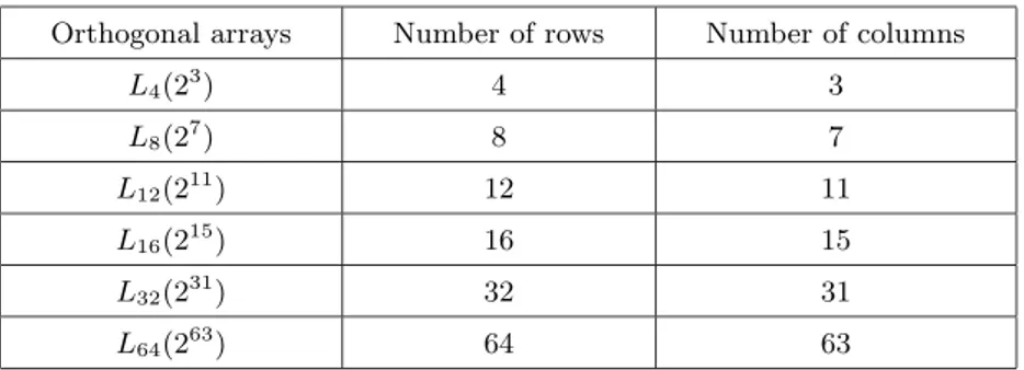
The 2-level orthogonal arrays in Taguchi’s catalogue (see [9]), and the number of runs (rows), factors and interactions (columns) are given in Table 2.2 [6,3,5].

Table 2.2. The 2-Level Orthogonal Arrays of Taguchi. Orthogonal arrays Number of rows Number of columns

L4(23) 4 3 L8(27) 8 7 L12(211) 12 11 L16(215) 16 15 L32(231) 32 31 L64(263) 64 63

In 2-level orthogonal arrays, each column has one degree of freedom and the number of rows must be at least the degree of freedom of the experiment [7,6].

For example, in an experiment with 7 factors each having 2 levels, if only the main factors are to be determined, the total degree of freedom of the experiment is 8. That is, one for the average and 7 for the 7 factors with 2 levels. Therefore, the smallest orthogonal array that can be used is L8(27), which has 8 rows and 7 columns.

The orthogonal array LN(2k) can be considered as an N/2k fraction of a complete

factorial plan in k factors, each having 2 levels [7,3]. For example; L4(23) in Table 2.2 is

the 4/8 = 1/2 fraction of the complete 23 _{factorial experiment.}

3. Triangular Tables

Taguchi [9] developed triangular tables, which give information about the columns of orthogonal arrays in interaction, in order to help with the design of experiments where interactions can be estimated. In Table 3.1, the triangular table corresponding to the orthogonal array L4 is given. The numbers in each row and column show the column

numbers in L4 (See Table 2.1). As an interaction between two columns a and b is

commutative, the triangular table is a symmetric matrix. Therefore, only the upper triangular part is given and lower triangular part is left blank in matrix representations.

Table 3.1. The Triangular Table for L4.

Column

Column 1 2 3

1 (1) 3 2

2 (2) 1

3 (3)

For example, using Table 3.1, assume factor A is assigned to the 1st column and factor B to to the 2nd column in L4. Then the triangular table of L4shows that column

3 contains the interaction between columns 1 and 2. A triangular table gives all the information necessary to assign factors to an orthogonal array in such a way as to obtain estimations of all the main effects and some of the desired interactions. Triangular tables for all 2nd order orthogonal arrays are given by Taguchi [9].

The usage of triangular table for orthogonal arrays of higher dimension is the same as that described for L4, the higher dimensional triangular tables in fact extending the

lower dimensional ones. For example the triangular table for L8 given in Table 3.2 also

contains the L4 triangular table [7,6].

Table 3.2. The Triangular Table for L8.

Column Column 1 2 3 4 5 6 7 1 (1) 3 2 5 4 7 6 2 (2) 1 6 7 4 5 3 (3) 7 6 5 4 4 (4) 1 2 3 5 (5) 3 2 6 (6) 1 7 (7)

4. Construction of Orthogonal Arrays

Taguchi [9] used the LN(sk) notation for orthogonal arrays, and pointed out that these

arrays may be constructed from Latin squares. A Latin square is a s × s dimensional square matrix, in the columns and rows of which each symbol appears only once. Two Latin squares L1 and L2of the same size are said to be orthogonal if all the s2pairs are

different when the two matrices are superimposed. Taguchi [9] states that an orthogonal array of size sr_{, (r = 2, 3, . . .), having (s}r_{− 1)/(s − 1) columns, can be formed from a}

Latin square of dimension s × s.

For example, in order to form L4(23), a 2 × 2 dimensional Latin square L is used

(Figure 4.1). Figure 4.1. Construction ofL4(23). L Column Row 1 2 1 1 2 2 2 1 −→ L4(23) Column Row 1 2 3 1 1 1 1 2 1 2 2 3 2 1 2 4 2 2 1

The rows of L4(23) (the runs) are formed from a row index, a column index and

the corresponding element of the Latin square L. For example, the first run of L4(23),

namely 111, is produced from the index 1 of the first row, the index 1 of the first column and the corresponding element 1 of L. With the same logic the value 2 at the second row and first column of L gives the row 212 of L4(23).

5. Linear Graphs

Taguchi [9] also proposed the method of linear graphs as an alternative to trian-gular tables to assign factors and interactions to orthogonal arrays. A linear graph is the graphical representation of some interactional relationships among the columns of an orthogonal array. Linear graphs are composed of nodes (vertices) and lines (edges. Numbers beside the vertices and edges of a linear graph represent the columns of the corresponding orthogonal array. Each vertex shows the assignment of a factor and each edge shows the column assigned to the interaction between the two factors corresponding to the vertices it is connecting. The total number of vertices and edges in a linear graph is equal to the number of columns in the orthogonal array. Every column of the orthogonal array is represented in the linear graph exactly once [9,3,5].

Figure 5.1. Linear Graph forL4

ÂÁÀ¿

»¼½¾

1 3

ÂÁÀ¿

»¼½¾

2

There is only one linear graph associated with L4. In Figure 5.1, the two vertices

correspond to columns 1 and 2. The line labelled 3 shows that column 3 contains the interaction between columns 1 and 2.

When the number of vertices and edges increase, the linear graph becomes more complex. There are 2 linear graphs for L8(Figure 5.2), and these are more complex than

that for L4. From linear graph no (I) in Figure 5.2, the interaction between the 1st and

2nd columns is in the 3rd column; the interaction between the 1st and 4th columns is in the 5th. However, no information about the interaction between the 1st and 7th column

can be gained. Such information can only be shown on the triangular table [6,5] The triangular table for L4 (See Table 3.1) shows the relations that cannot be seen on Figure

5.2.

Figure 5.2. Linear Graphs forL8

(I)

ÂÁÀ¿

»¼½¾

1 3 ~~~~ ~~~~ ~~ 5 @ @ @ @ @ @ @ @ @ @

ÂÁÀ¿

»¼½¾

7

ÂÁÀ¿

»¼½¾

2 6

ÂÁÀ¿

»¼½¾

4 (II)

ÂÁÀ¿

»¼½¾

2

ÂÁÀ¿

»¼½¾

1 3_jjjjjj j j j j j j j 5 6TTTTT_TT T T T T T T

ÂÁÀ¿

»¼½¾

4

ÂÁÀ¿

»¼½¾

7

The reason for giving more than one linear graph for an orthogonal array is to allow the construction of different experimental designs. For example, if all the interaction to be estimated contain a common factor (A × B, A × C, A × D) then linear graph no II is appropriate, if the expected interactions contain each factor twice (A × B, B × C, A × C), then linear graph no I shall be selected [9,5].

6. Some Basic Definitions on the usage of Linear Graphs

A graph is a set of points and lines. These points and lines have no attributes: lengths and positions are not important. Generally the terms vertex and edge are used instead of point and line, respectively [4].

6.1. Definition. A graph consists of a finite set vertices and edges. The symbol G(e, v) is used for a graph with e edges and v vertices. Some special graphs are shown using capital letters with subscripts, such as G1, G2 [4].

6.2. Definition. A vertex of a graph may be represented by a point, small circle or filled node in the plane.

6.3. Definition. An edges of a graph may be represented by a line joining two of the vertices.

6.4. Definition. When a vertex and an edge are connected they are said to be incident. 6.5. Definition. The number of edges incident with a vertex is called its degree.

In Figure 6.1 (I), the edges 1 and 2 are incident with vertex a. In Figure 6.1 (II), as there are two edges incident with vertex d, the degree of vertex d is 2.

Figure 6.1. Elements of a Graph (I)

ÂÁÀ¿

»¼½¾

b 3 2 ªªªª ªªªª ªª 6 * * * * * * * * * * * * * * * * * 8 O O O O O O O O O O O O O O O O O O O

ÂÁÀ¿

»¼½¾

c 7 oooooo oooooo oooooo o 9 ··· ··· ·· ··· ··· ··· · 4 5 5 5 5 5 5 5 5 5

ÂÁÀ¿

»¼½¾

a 10 1 H H H H H H H H H H H H H

'&%$

Ã!"#

d 5 vvvv vvvv vvvv v

ÂÁÀ¿

»¼½¾

e (II)

ÂÁÀ¿

»¼½¾

a 2 3 K K K K K K K K K K K K K K K 1

ÂÁÀ¿

»¼½¾

b

ÂÁÀ¿

»¼½¾

c 4

'&%$

Ã!"#

d

ÂÁÀ¿

»¼½¾

e 5

'&%$

Ã!"#

f

6.6. Definition. Two edges incident with the same vertex are called incident edges. In Figure 6.1 (II) edges 3 and 4, which are incident to vertex d, are incident edges.

6.7. Definition. Two vertices incident to the same edge are called incident vertices. In Figure 6.1 (II), vertices a and b, which are incident to edge 2, are incident vertices [4].

6.1. Isomorphic Graphs. Wu and Chen [10] describe a graph constant, the degree sequence, to test the isomorphism of graphs. The degree sequence, d = (d1, d2, . . . , dv),

where the di ’s are the degrees in descending order of the v vertices of the graph, is

a graph-invariant. For example the degree sequence of the graph in Figure 6.2 is d = (4, 3, 2, 2, 1). Note that, although there are 6 vertices of this graph only 5 degrees are given, the 6th vertex being an isolated vertex (a vertex of degree 0, with no incident edges). Isolated vertices are not shown in a degree sequence as their degrees are 0 [1,10].

Figure 6.2. Vertex Degrees of a Graph

ÂÁÀ¿

»¼½¾

3 @ @ @ @ @ @ @ @ @ @ @

ÂÁÀ¿

»¼½¾

2

ÂÁÀ¿

»¼½¾

1 ~~~~ ~~~~ ~~~

ÂÁÀ¿

»¼½¾

4

ÂÁÀ¿

»¼½¾

5

ÂÁÀ¿

»¼½¾

6

Two graphs having the same degree sequence are not necessarily isomorphic, but if two graphs have different degree sequences they cannot be isomorphic. To check isomorphism, for each vertex i, define its extended degree to be Di = P dij, where the dij are the

degrees of all vertices incident to i. Two graphs with the same degree sequences are isomorphic if their extended degrees, Di, are equivalent [10].

There are binary operations like intersection and conjunction defined on graphs, but here only 2 binary operations will be described [8].

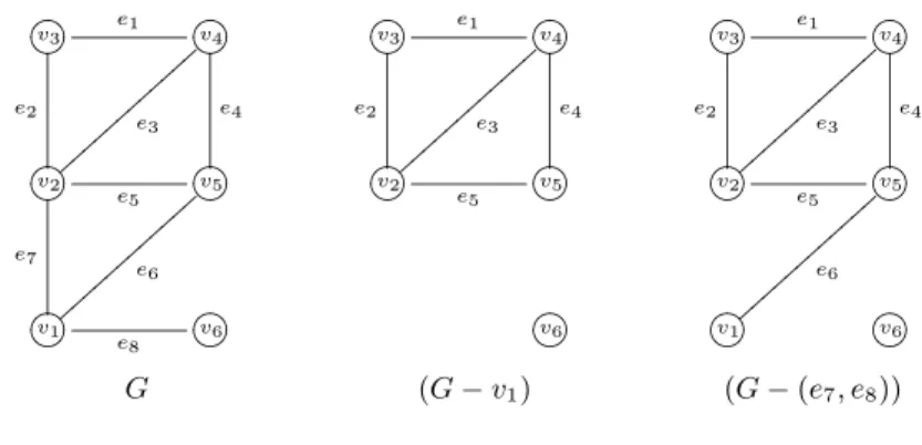
1. Vertex Removal: Let vi be a vertex of the graph G(e, v). The graph formed by

removing viand all incident edges is denoted by (G − vi). This graph is a subset of G.

If v1and all incident edges are removed from the graph G in Figure 6.3, the subgraph

(G − v1) shown in Figure 6.3 is found.

2. Edge Removal: Let eibe an edge of the graph G(e, v). The graph formed by removing

eiis denoted by (G − ei). This graph is a subset of G. In edge removal, incident vertices

are not removed from the graph G.

The graph (G − (e7, e8)) in Figure 6.3 is obtained from G by removing the edges e7

and e8. The vertices v1, v2and v6, which are incident to e7and e8, are not removed from

the graph [8].

Figure 6.3. Two Operations on a Graph

'&%$

Ã!"#

v3 e1 e2

'&%$

Ã!"#

v4 e3 |||| |||| |||| e4

'&%$

Ã!"#

v2 e5 e7

'&%$

Ã!"#

v5 e6 |||| |||| ||||

'&%$

Ã!"#

v1 e8

'&%$

Ã!"#

v6

'&%$

Ã!"#

v3 e1 e2

'&%$

Ã!"#

v4 e3 |||| |||| |||| e4

'&%$

Ã!"#

v2 e5

'&%$

Ã!"#

v5

'&%$

Ã!"#

v6

'&%$

Ã!"#

v3 e1 e2

'&%$

Ã!"#

v4 e3 |||| |||| |||| e4

'&%$

Ã!"#

v2 e5

'&%$

Ã!"#

v5 e6 |||| |||| ||||

'&%$

Ã!"#

v1

'&%$

Ã!"#

v6 G (G − v1) (G − (e7, e8))

7. Assignment of Factors and Interactions to Linear Graphs

Taguchi’s approach to the assignment of factors and interactions to the columns using orthogonal arrays consists of the following steps [3,5].

1. According to a list of expected factors of an experiment, named by Taguchi [9] the requirement set, the smallest orthogonal array that could yield an experiment capable of estimating the effects listed in the requirement set is chosen. The degree of freedom of the experiment is calculated and compared with the degree of freedom of the orthogonal array.

2. Using the requirement set; by representing the main factors by vertices and the interactions as edges connecting the vertices, a graph similar to a linear graph is drawn. Taguchi [9] names this graph required linear graph.

3. Using to orthogonal array determined in step 1, the linear graph of this array that most resembles the required linear graph is selected.

4. The selected linear graph is used to assign factors and interactions to the columns of the orthogonal array. If the required linear graph and the selected linear graph are isomorphic, this assignment can be done easily using the one to one relation between the graphs. However, as the required linear graph depends on the requirement set, this may not always be possible.

5. If there are factor changes involving different levels, isomorphic graphs of the selected linear graph can be examined to compare column assignments.

As an example, assume that we have an experiment where the assignments will be made to estimate the main factors A, B, C, D and the interactions A × B, B × C and A × C. Following the steps described above:

1. As the requirement list contains 4 main factors and 3 interactions, the degree of freedom of this experiment is 4+3=7. The smallest orthogonal array with which these parameters can be estimated is L8, whose degree of freedom is 7

(See Table 2.2).

2. Using the requirement set {A, B, C, D, A × B, A × C, B × C}, the required linear graph is as given below, where the main factors and interactions are shown as vertices and edges respectively.

'&%$

Ã!"#

A A×B }}}} }}}} }} A×C A A A A A A A A A A

'&%$

Ã!"#

D

'&%$

Ã!"#

B B×C

'&%$

Ã!"#

C

3. The selection of the linear graph most similar to the required linear graph is done among the linear graphs of L8(Figure 5.2). Clearly linear graph number I

is isomorphic to the required linear graph.

ÂÁÀ¿

»¼½¾

1 3 ~~~~ ~~~~ ~~ 5 @ @ @ @ @ @ @ @ @ @

ÂÁÀ¿

»¼½¾

7

ÂÁÀ¿

»¼½¾

2 6

ÂÁÀ¿

»¼½¾

4

4. Using the required linear graph and linear graph number I of L8, the assignments

to L8 are made. Firstly D is assigned to column 7. As both graphs contains

columns, and the interactions A × B, B × C and A × C are assigned to the 3rd, 5th and 6th columns, respectively.

A↔1 A×B↔3 ¡¡¡¡ ¡¡¡¡ ¡¡¡¡ ¡ A×C↔5 > > > > > > > > > > > > > D↔7 B↔2 B×C↔6 C↔4

5. As there is no factor whose degree is difficult to change, this step is unnecessary. Moreover no isomorphic graphs are given for the linear graphs of L8. However if

we had such an assumption on factor C, it could be assigned to the 1st column instead of the 4th.

The experiment whose assignments are obtained step by step as above in an easy example given to explain how linear graphs are used with only 4 factors and 3 interactions. Unfortunately, the assignment of factors and interactions to linear graphs is not always that easy. In most cases, some operations on the linear graphs are needed.

7.1. Modification of Linear Graphs. In applications, especially in experiments where L16or higher level orthogonal arrays are used, and the number or factors and interactions

increases, the linear graphs may need to be modified. There are 3 methods to modify linear graphs for 2 level orthogonal arrays.

1. Edge split: In a linear graph, an edge that connects two vertices can be removed and replaced by a vertex. As can be seen from Figure 7.1(I), edge number 7 can be removed from the graph. Although in graph theory a removed edge does not appear in the graph, it is retained here as a vertex. The reason for this is that each vertex and edge in the linear graph corresponds to a row in the orthogonal array. As removing edge number 7 from the graph means to remove a column from the array, it is taught that Taguchi preferred to replace it with a vertex.

2. Edge forming: An edge can be added to a linear graph by connecting two vertices. In Figure 7.1 (III) there are 3 vertices; 1, 4 and 5, which can be a part of the linear graph of L8 or a higher level orthogonal array. Here vertex number 5 is changed to an edge

connecting the vertices 1 and 4. Such a combination can be formed by using triangular tables. Assuming these vertices belong to the linear graph of L8, from the triangular

table of L8 it can be seen that the interaction between columns 1 and 4 is in the 5th

column. In Figure 7.1 (II) the vertex that will be changed to edge also could have been 1 or 4, because from the triangular table of L8 it can be seen that the interaction between

columns 4 and 5 is in the 1st column and the interaction between columns 1 and 5 is in 4th column. In conclusion, while forming the edges, attention should be paid to the consistency of the column assignments with the triangular table [6-5].

3. Edge moving: An edge connected to two vertices can be moved to connect two other vertices. In Figure 7.1 (III), edge 3 which is incident to vertices 1 and 2 can be moved to connect vertices 5 and 6. However for such a move to be possible, the interaction between 5 and 6 must be on 3rd column too (See Table 3.2). To decide this, the triangular table of L8 is used.

When a modification of the linear graph is necessary, the following steps for the assignment of factor and interactions are suggested.

(1) The smallest orthogonal array large enough to estimate the factors and interac-tions in the experiment is selected.

(2) The required linear graph is drawn using the requirement set.

(3) The linear graph which most closely resembles the required linear graph is se-lected from among the linear graphs of the orthogonal array.

(4) The required linear graph and the selected linear graph are matched. The factors and interactions are assigned. If all the interactions can be assigned, step 5 is skipped.

(5) To complete the assignment of the interactions, the linear graph modification methods are applied using the triangular tables.

(6) Alternates or isomorphs of the linear graphs are compared [5]. Figure 7.1. Modification of Linear Graphs (I) Edge Split

ÂÁÀ¿

»¼½¾

1 3

7

ÂÁÀ¿

»¼½¾

2

ÂÁÀ¿

»¼½¾

6 =⇒

»¼½¾

ÂÁÀ¿

1 3

ÂÁÀ¿

»¼½¾

2

ÂÁÀ¿

»¼½¾

6

ÂÁÀ¿

»¼½¾

7

(II) Edge Forming

ÂÁÀ¿

»¼½¾

1

ÂÁÀ¿

»¼½¾

4

»¼½¾

ÂÁÀ¿

5 =⇒

ÂÁÀ¿

»¼½¾

1 5

ÂÁÀ¿

»¼½¾

4

(III) Edge Moving

ÂÁÀ¿

»¼½¾

1 3

ÂÁÀ¿

»¼½¾

2

ÂÁÀ¿

»¼½¾

5

ÂÁÀ¿

»¼½¾

6

=⇒

»¼½¾

ÂÁÀ¿

1

ÂÁÀ¿

»¼½¾

2

ÂÁÀ¿

»¼½¾

5 3

ÂÁÀ¿

»¼½¾

6

The following example illustrates these steps. Suppose that an experiment has 10 main factors A, B, C, D, E, F , G, H, I and J, and that we want to estimate the factors A × B, B × C, C × E, D × E and D × F .

1. First, as the requirement set has 10 main factor and 5 interactions, the degree of freedom of the experiment is 10 + 5 = 15. The smallest orthogonal array that can be used to estimate these effects is L16, whose degree of freedom is 15.

2. Using the requirement set the required linear graph is drawn:

'&%$

Ã!"#

A

'&%$

Ã!"#

C

'&%$

Ã!"#

D

'&%$

Ã!"#

G

'&%$

Ã!"#

H

'&%$

Ã!"#

I

'&%$

Ã!"#

J

'&%$

Ã!"#

B ± ± ± ± ± ± ± ± ± ± ± ±

_'&%$

_Ã!"#

E ° ° ° ° ° ° ° ° ° ° ° °

_'&%$

_Ã!"#

F

3. As the orthogonal array L16 has been chosen, the choice of linear graph will be made

among the linear graphs of L16 (see [9]). The graph in Taguchi’s catalogue most similar

to the required linear graph is (V):

'&%$

Ã!"#

1 3

'&%$

Ã!"#

4 12

'&%$

Ã!"#

5 15

'&%$

Ã!"#

14 3

'&%$

Ã!"#

6 13

'&%$

4. When we compare the required graph with the linear graph, in order to have no unassigned factors or interactions, the two graphs should be isomorphic. Using the concept of degree sequence described in section 6.1, the degree sequence of the required graph is found as dRLG= (2, 2, 2, 2, 1, 1). As the required linear graph has four isolated

vertices, these are not included in the degree sequence. As the degree sequence of the Number (V) linear graph of L16is dLG= (1, 1, 1, 1, 1, 1, 1, 1, 1, 1), which is different from

dRLG, the two graphs are not isomorphic. Hence all assignments cannot be made.

5. The linear graph is modified in two steps to make it isomorphic to the required linear graph so that the assignments could be made.

In Step I, using edge splitting as described in 7.1, edge 14 connecting the vertices 6 and 11 and edge 13 connecting the vertices 6 and 11 are removed and placed in the graph as vertices. Step I

'&%$

Ã!"#

1 3

'&%$

Ã!"#

4 12

'&%$

Ã!"#

5

15

'&%$

Ã!"#

6

'&%$

Ã!"#

7

'&%$

Ã!"#

9

'&%$

Ã!"#

11

'&%$

Ã!"#

13

'&%$

Ã!"#

14

'&%$

Ã!"#

2

'&%$

Ã!"#

8

'&%$

Ã!"#

10

In Step II, using the edge forming method, vertex 6 is converted to an edge connecting vertices 2 and 4, and vertex 13 is converted to an edge connecting vertices 5 and 8. In the triangular table of the L16(see [9]), the interaction between the 2nd and 4th columns is

in the 6th, and the interaction between the 5th and 8th columns is in the 13th, so these edges are attached to the graph. The modified linear graph of L16 after the addition of

the edges 6 and 13 is: Step II

'&%$

Ã!"#

1 3

'&%$

Ã!"#

4 12

'&%$

Ã!"#

5 15

'&%$

Ã!"#

7

'&%$

Ã!"#

9

'&%$

Ã!"#

11

'&%$

Ã!"#

14

'&%$

Ã!"#

2 6 ² ² ² ² ² ² ² ² ² ² ² ² ² ²

'&%$

Ã!"#

8 13 ± ± ± ± ± ± ± ± ± ± ± ± ± ±

'&%$

Ã!"#

10

which is isomorphic to the required linear graph. Hence the using the one to one relation between these graphs, the assignment of factors and interactions can be done directly:

1↔A 3↔A×B 4↔C 12↔C×E 5↔D 15↔D×F 7↔G 9↔H 11↔I 14↔J 2↔B 6↔B×C_°°° ° ° ° ° ° ° ° ° ° ° ° ° ° ° ° ° 8↔E 13↔D×E_°°° ° ° ° ° ° ° ° ° ° ° ° ° ° ° ° ° 10↔F

6. As the orthogonal array is L16, there are three alternative assignments for each linear

graph. However as there is no restrictions on the factors of the experiment there is no need to check for isomorphs [2].

8. Conclusion

When forming a 2-level fractional factorial experiment using orthogonal arrays, the lin-ear graph and triangular table methods of Taguchi supports the design visually. Provided we have a requirement set, drawing the required linear graph helps with the determina-tion of which linear graph enable the assignments to be made, or helps with the selecdetermina-tion of this linear graph using the isomorphic property.

References

[1] Behzad, M. and Chartrand, G. Introduction to the Theory of Graphs, (Boston, Allyn and Bacon, Boston, 271p., 1971).

[2] Danacıo˘glu, N. A Comparison of Constructions Methods of Orthogonal Arrays used in Taguchi Designs, (H. U. Department of Statistics, MSc Thesis (in Turkish), 1999). [3] Kacker, R. N. and Tsui, K. L. Interaction graphs: graphical aids for planning experiments,

J. Qual. Technol. 22 (1), 1–14, 1990.

[4] Maxwell, L. M. and Reed, M. B. The Theory of Graphs: A basis for Network Theory, Perg-amon Press, New York, 164p, 1971).

[5] Peace, G. S. Taguchi Methods: A Hands-On Approach, (Addison-Wesley Publishing Com-pany, Reading. M.A., USA, 1993).

[6] Phadke, M. S. Quality Engineering using Robust Design, (AT&T Bell Labarotories, Engle-wood Cliffs, New Jersey, 334 p, 1999).

[7] Ross, P. J. Taguchi Techniqes for Quality Engineering: Loss Function Orthogonal Experi-ments, Parameter and Tolerance Design, (Mc Graw-Hill Book Company, New York, 1998). [8] Swamy, M. N. S. and Thulasiraman, K. Graphs, Networks and Algorithms, (Wiley. New

York., 592 p., 1981).

[9] Taguchi, G. System of Experimental Design: Engineering Methods to Optimize Quality and Minimize Costs, (UNIPUB/Kraus International Publications - Two Volumes, 1987). [10] Wu, C. F. J. and Chen, Y. Y. A graph-aided method for planning two-level experiments when