Başlık: A software tool for retrieving land surface temperature from ASTER imageryYazar(lar):OĞUZ, HakanCilt: 21 Sayı: 4 Sayfa: 471-482 DOI: 10.1501/Tarimbil_0000001350 Yayın Tarihi: 2015 PDF

(1)

Tarım Bilimleri Dergisi

Tar. Bil. Der.

Dergi web sayfası: www.agri.ankara.edu.tr/dergi

Journal of Agricultural Sciences

Journal homepage: www.agri.ankara.edu.tr/journal

TARIM BİLİMLERİ DERGİSİ

—

JOURNAL OF AGRICUL

TURAL SCIENCES

21 (2015) 471-482

A Software Tool for Retrieving Land Surface Temperature from

ASTER Imagery

Hakan OĞUZa

a_{Kahramanmaraş Sütçü İmam University, Faculty of Forestry, Department of Landscape Architecture, 46100, Kahramanmaraş, TURKEY}

ARTICLE INFO

Research Article

Corresponding Author: Hakan OĞUZ, E-mail: hakan@ksu.edu.tr, Tel: +90 (344) 280 18 13

Received: 22 April 2014, Received in Revised Form: 11 September 2014, Accepted: 20 September 2014

ABSTRACT

Remote sensing is a powerful and well-known tool in the collection, analysis, and modeling of environmental data, however, not much attention has been given to the use of thermal infrared (TIR) remote sensing. Land surface temperature (LST) is a key parameter for many environmental studies such as global environmental change, climate models, and human-environment interactions. In this study, a software tool which retrieves LST from Advanced Spaceborne Thermal Emission and reflection Radiometer (ASTER) imagery has been developed in Visual Basic .NET. The tool consists of five main modules: 1- Converting DN to Radiances, 2- Calculating surface reflectances, 3- Calculating NDVI, 4- Calculating emissivity and 5- Calculating surface temperature. In this tool, Jimenez Munoz and Sobrino’s Single Channel (SCJM&S_{) Algorithm for ASTER was employed. With this tool, user can be able to calculate LST using (1)}

atmospheric parameters such as atmospheric transmissivity, upwelling and downwelling atmospheric radiances, (2) atmospheric water-vapor content. Hopefully, this program will be a useful tool for scientists/persons who are interested in studying thermal environments.

Keywords: Urban climate; Urban heat island; Thermal infrared remote sensing; Atmospheric parameters; Water-vapor content; Visual Basic.NET

ASTER Uydu Görüntüsünden Yer Yüzey Sıcaklığını Hesaplayan Bir

Yazılım Aracı Geliştirilmesi

ESER BİLGİSİ

Araştırma Makalesi

Sorumlu Yazar: Hakan OĞUZ, E-posta: hakan@ksu.edu.tr, Tel: +90 (344) 280 18 13 Geliş Tarihi: 22 Nisan 2014, Düzeltmelerin Gelişi: 11 Eylül 2014, Kabul: 20 Eylül 2014

ÖZET

Çevresel verinin toplanması, analizi ve modellemesinde uzaktan algılama çok önemli ve iyi bilinen bir araç olmasına rağmen, termal kızılötesi (TIR) uzaktan algılamasına gereken önem verilmemiştir. Küresel çevre değişimi, iklim modelleri ve insan-çevre etkileşimleri gibi birçok çevresel çalışmalar için yer yüzey sıcaklığı (LST) önemli bir parametredir. Bu çalışmada, Visual Basic NET programlama dili kullanılarak ASTER uydu görüntüsünden yer yüzey sıcaklığını

(2)

A Software Tool for Retrieving Land Surface Temperature from ASTER Imagery, Oğuz

472

Ta r ı m B i l i m l e r i D e r g i s i – J o u r n a l o f A g r i c u l t u r a l S c i e n c e s 21 (2015) 471-482

1. Introduction

Urban heat island effect, global warming, enhanced green-house effects and other environmental problems have become very important subjects to overcome in the last decades. Land surface temperature is an important parameter for many environmental models (Xiao et al 2007). LST retrieval using remotely sensed data is the most popular subjects in environmental studies during the last couple of decades (Genc et al 2010).

The ASTER on the NASA’s Terra platform is the highest spatial resolution with 90 m multispectral TIR sensor currently available on a polar-orbiting spacecraft. The accuracies for temperature and emissivity separation (TES) algorithm were found to be within the specifications of ±0.015 for emissivity and ±1.5 K for LST. However, some inaccuracies have been found over agricultural areas. These problems were pointed out in Gillespie et al (1998) and have been explicitly analyzed and those problems were partially avoided over agricultural areas by Jimenez-Munoz et al (2006); Gustafson et al (2006) and Sobrino et al (2007). Another method was developed by Jimenez-Munoz & Sobrino (2007) using split-window (SW) algorithms to retrieve LST from ASTER imagery, where input emissivities can be calculated from the normalized difference vegetation index (NDVI) (Jimenez-Munoz et al 2006). Results retrieved from this methods howed similar errors to those specified for TES products.

Currently, there are two programs developed for LST retrieval from Landsat imagery (Zhang et al 2006; Oguz 2013), however, no software tools were developed for ASTER imagery yet. Therefore, in

this particular study, a program was developed in order to retrieve LST from ASTER imagery. In this tool, a single-channel (SC) algorithm developed by Jimenez-Munoz & Sobrino (2010) was employed, which was oriented for people who:

- are interested in LST retrieval but not familiar with TES products

- cannot get TES products, or

- have found unsatisfactory results by using TES products, so prefer another method different than the SW algorithm mentioned earlier. This algorithm is easy to implement and also based on the procedure formulated by Jimenez-Munoz & Sobrino (2003). It has been designed for ASTER satellite imagery based on the algorithm developed for Landsat TIR imagery (Jimenez-Munoz et al 2009). The algorithm is hereinafter denoted as SCJM&S_.

2. Material and Methods

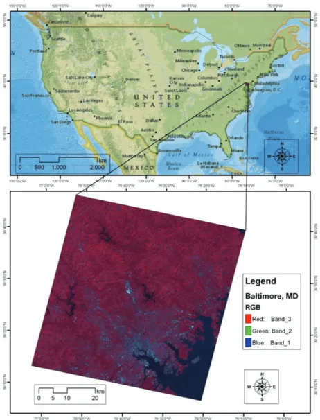
2.1. ASTER imagery

The ASTER was launched on NASA’s Terra spacecraft in 1999, and each scene contains 14 bands from visible to thermal infrared region with coverage of 60 x 60 km area. ASTER contains three different band groups (Table 1); in the first group, there are four bands within the Visible and Near-infrared (VNIR) region with a spatial resolution of 15 m; in the second group, there are six bands in the Shortwave Infrared (SWIR) region with a spatial resolution of 30 m and in the third and final group, there are five bands within TIR region with a spatial resolution of 90 m (Abrams et al 2008).

hesaplayan bir yazılım aracı geliştirilmiştir. Bu araç beş modülden oluşmaktadır: 1- Dijital Sayıları (DN) Radyansa dönüştürme, 2- Yüzey yansıma değerinin hesaplanması, 3- NDVI’ın hesaplanması, 4- Yayınırlığın hesaplanması ve 5- Sıcaklığın hesaplanması. Bu yazılım aracında Jimenez Munoz ve Sobrino’nun ASTER uydu görüntüsünden yer yüzey sıcaklığının hesaplanması için geliştirdiği Tek Kanal (Single Channel) Algoritması kullanılmıştır. Bu programın termal çevre üzerine çalışan bilim insanları veya konuyla ilgilenen kişiler için faydalı olabileceği ümit edilmektedir.

Anahtar Kelimeler: Kentsel iklim; Kentsel ısı adası; Termal kızılötesi uzaktan algılaması; Atmosferik parametreler; Su buharı içeriği; Visual Basic NET

(3)

ASTER Uydu Görüntüsünden Yer Yüzey Sıcaklığını Hesaplayan Bir Yazılım Aracı Geliştirilmesi, Oğuz

473

Ta r ı m B i l i m l e r i D e r g i s i – J o u r n a l o f A g r i c u l t u r a l S c i e n c e s 21 (2015) 471-482 The single-channel (SCJM&S_{) algorithm}

The SCJM&S_{algorithm calculates LST (T} S) using the Equation 1.

2

Table 1- Characteristics of the ASTER sensor systems (Abrams et al 2008) Çizelge 1- ASTER sensör sistemlerinin özellikleri (Abrams et al 2008)

Subsystem Band number Spectral range (μm) Spatial resolution (m) Quantization levels VNIR 1 0.52 – 0.60 15 8 bits 2 0.63 – 0.69 3N 0.78 – 0.86 3B 0.78 – 0.86 SWIR 4 1.60 – 1.70 30 8 bits 5 2.145 – 2.185 6 2.185 – 2.225 7 2.235 – 2.285 8 2.295 – 2.365 9 2.360 – 2.430 TIR 10 8.125 – 8.475 90 12 bits 11 8.475 – 8.825 12 8.925 – 9.275 13 10.25 – 10.95 14 10.95 – 11.65

The single-channel (SCJM&S_{) algorithm}

The SCJM&S_{algorithm calculates LST (T}_S_{) using the equation 1.}

𝑇𝑇𝑇𝑇𝑠𝑠𝑠𝑠= γ[(1 𝜀𝜀𝜀𝜀⁄ )(𝜓𝜓𝜓𝜓1𝐿𝐿𝐿𝐿𝑠𝑠𝑠𝑠𝑠𝑠𝑠𝑠𝑠𝑠𝑠𝑠+ 𝜓𝜓𝜓𝜓2) + 𝜓𝜓𝜓𝜓3] + 𝛿𝛿𝛿𝛿 (1)

Where; ε is the surface emissivity; 𝐿𝐿𝐿𝐿𝑠𝑠𝑠𝑠𝑠𝑠𝑠𝑠𝑠𝑠𝑠𝑠is the at-sensor registered radiances; γ and δ are two parameters

dependent on the Planck’s equation, and 𝜓𝜓𝜓𝜓1, 𝜓𝜓𝜓𝜓2and 𝜓𝜓𝜓𝜓3are referred to as atmospheric parameters (AP) and

given in equation 2.

𝜓𝜓𝜓𝜓1= (1 𝜏𝜏𝜏𝜏⁄ ), 𝜓𝜓𝜓𝜓2= −𝐿𝐿𝐿𝐿↓− �𝐿𝐿𝐿𝐿↑⁄ �, 𝜓𝜓𝜓𝜓𝜏𝜏𝜏𝜏 3= 𝐿𝐿𝐿𝐿↓ (2)

Where; 𝜏𝜏𝜏𝜏 is the atmospheric transmissivity; 𝐿𝐿𝐿𝐿↑ _{is the upwelling atmospheric radiance, and 𝐿𝐿𝐿𝐿}↓ _{is the}

downwelling atmospheric radiance. It is also essential to convert at-sensor registered radiances (𝐿𝐿𝐿𝐿𝑠𝑠𝑠𝑠𝑠𝑠𝑠𝑠𝑠𝑠𝑠𝑠) into

at-sensor brightness temperatures (Tsen) especially when working with thermal bands. Tsen is computed using

inversion of the Planck’s law (Jimenez-Munoz & Sobrino 2010) and presented in equation 3.

𝑇𝑇𝑇𝑇𝑠𝑠𝑠𝑠𝑠𝑠𝑠𝑠𝑠𝑠𝑠𝑠= 𝐾𝐾𝐾𝐾2 ln �_{𝐿𝐿𝐿𝐿}𝐾𝐾𝐾𝐾1

𝑠𝑠𝑠𝑠𝑠𝑠𝑠𝑠𝑠𝑠𝑠𝑠+ 1�

� (3)

Where; K1and K2are the radiation constants which are given in Table 2.

Table 2- Radiation constants used in equation 3

Çizelge 2- Denklem 3’te kullanılan radyasyon sabit değerleri

ASTER Band K1(W m2sr-1μm-1) K2(K) 10 3047.47 1736.18 11 2480.93 1666.21 12 1930.80 1584.72 13 865.65 1349.82 14 649.60 1274.49 (1) Where; ε is the surface emissivity; is the at-sensor registered radiances; γ and δ are two parameters dependent on the Planck’s equation, and

2

� (3)

ASTER Band K1(W m2sr-1μm-1) K2(K) 10 3047.47 1736.18 11 2480.93 1666.21 12 1930.80 1584.72 13 865.65 1349.82 14 649.60 1274.49 and

2

𝑇𝑇𝑇𝑇𝑠𝑠𝑠𝑠 = γ[(1 𝜀𝜀𝜀𝜀⁄ )(𝜓𝜓𝜓𝜓1𝐿𝐿𝐿𝐿𝑠𝑠𝑠𝑠𝑠𝑠𝑠𝑠𝑠𝑠𝑠𝑠+ 𝜓𝜓𝜓𝜓2) + 𝜓𝜓𝜓𝜓3] + 𝛿𝛿𝛿𝛿 (1)

� (3)

ASTER Band K1(W m2sr-1μm-1) K2(K) 10 3047.47 1736.18 11 2480.93 1666.21 12 1930.80 1584.72 13 865.65 1349.82 14 649.60 1274.49

are referred to as atmospheric parameters (AP) and given in Equation 2.

2

Where; ε is the surface emissivity; 𝐿𝐿𝐿𝐿𝑠𝑠𝑠𝑠𝑠𝑠𝑠𝑠𝑠𝑠𝑠𝑠 is the at-sensor registered radiances; γ and δ are two parameters

dependent on the Planck’s equation, and 𝜓𝜓𝜓𝜓1, 𝜓𝜓𝜓𝜓2 and 𝜓𝜓𝜓𝜓3 are referred to as atmospheric parameters (AP) and

� (3)

ASTER Band K1(W m2sr-1μm-1) K2(K) 10 3047.47 1736.18 11 2480.93 1666.21 12 1930.80 1584.72 13 865.65 1349.82 14 649.60 1274.49 (2) Where; is the atmospheric transmissivity;

2

Where; ε is the surface emissivity; 𝐿𝐿𝐿𝐿𝑠𝑠𝑠𝑠𝑠𝑠𝑠𝑠𝑠𝑠𝑠𝑠 is the at-sensor registered radiances; γ and δ are two parameters

� (3)

ASTER Band K1(W m2sr-1μm-1) K2(K) 10 3047.47 1736.18 11 2480.93 1666.21 12 1930.80 1584.72 13 865.65 1349.82 14 649.60 1274.49

is the upwelling atmospheric radiance, and

2

� (3)

ASTER Band K1(W m2sr-1μm-1) K2(K) 10 3047.47 1736.18 11 2480.93 1666.21 12 1930.80 1584.72 13 865.65 1349.82 14 649.60 1274.49 is the downwelling atmospheric radiance. It is also essential to convert at-sensor registered radiances (L_sen) into at-sensor brightness temperatures (T_sen) especially when working with thermal bands. T_sen is computed using inversion of the Planck’s law (Jimenez-Munoz & Sobrino 2010) and presented in Equation 3.

2

� (3)

ASTER Band K1(W m2sr-1μm-1) K2(K) 10 3047.47 1736.18 11 2480.93 1666.21 12 1930.80 1584.72 13 865.65 1349.82 14 649.60 1274.49 (3) Where; K1 and K2 are the radiation constants which are given in Table 2.

Table 2- Radiation constants used in Equation 3 Çizelge 2- Eşitlik 3’te kullanılan radyasyon sabit değerleri ASTER Band K₁ (W m2_sr-1 _μm-1₎ _K 2 (K) 10 3047.47 1736.18 11 2480.93 1666.21 12 1930.80 1584.72 13 865.65 1349.82 14 649.60 1274.49

Parameters γ and δ used in Equation 1 can be calculated by Equation 4.

3

Parameters γ and δ used in equation 1 can be calculated by equation 4.

𝛾𝛾𝛾𝛾 ≈ (𝑇𝑇𝑇𝑇𝑠𝑠𝑠𝑠𝑠𝑠𝑠𝑠𝑠𝑠𝑠𝑠2 ⁄𝐾𝐾𝐾𝐾2𝐿𝐿𝐿𝐿𝑠𝑠𝑠𝑠𝑠𝑠𝑠𝑠𝑠𝑠𝑠𝑠), 𝛿𝛿𝛿𝛿 ≈ 𝑇𝑇𝑇𝑇𝑠𝑠𝑠𝑠𝑠𝑠𝑠𝑠𝑠𝑠𝑠𝑠− (𝑇𝑇𝑇𝑇𝑠𝑠𝑠𝑠𝑠𝑠𝑠𝑠𝑠𝑠𝑠𝑠2 ⁄ )𝐾𝐾𝐾𝐾2 (4)

Where; Tsenis computed using equation (3) and K2can be retrieved from Table 2.

Even though the APs can be computed in a number of different ways as explained by Jimenez-Munoz & Sobrino (2010), the SCJM&S_{method was selected and used in this particular study due to the fact that the}

model requires minimal and more accessible input data The atmospheric parameters; 𝜏𝜏𝜏𝜏, 𝐿𝐿𝐿𝐿↑_{, and 𝐿𝐿𝐿𝐿}↓ _{can be}

computed using the local atmospheric sounding and MODTRAN.

Atmospheric parameters can also be obtained from second-order polynomial fits versus the atmospheric water-vapor content (Jimenez-Munoz & Sobrino 2003; Jimenez-Munoz & Sobrino 2007; Jimenez-Munoz & Sobrino 2010) as shown in equation 5.

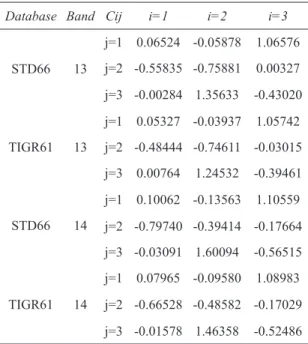
�𝜓𝜓𝜓𝜓𝜓𝜓𝜓𝜓12 𝜓𝜓𝜓𝜓3 � = �𝑐𝑐𝑐𝑐𝑐𝑐𝑐𝑐1121 𝑐𝑐𝑐𝑐𝑐𝑐𝑐𝑐1222 𝑐𝑐𝑐𝑐𝑐𝑐𝑐𝑐1323 𝑐𝑐𝑐𝑐31 𝑐𝑐𝑐𝑐32 𝑐𝑐𝑐𝑐33 � �𝜔𝜔𝜔𝜔 2 𝜔𝜔𝜔𝜔 1� (5)

Where; coefficients cij are obtained from simulated data constructed from atmospheric profiles as

described in Jimenez-Munoz & Sobrino (2010) (Table 3).

Table 3- Coefficients for the atmospheric functions following matrix notation in equation 5 (Jimenez-Munoz & Sobrino 2010)

Çizelge 3- Denklem 5’te kullanılan katsayı değerleri (Jimenez-Munoz & Sobrino 2010)

Database Band Cij i=1 i=2 i=3

STD66 13 j=1 0.06524 -0.05878 1.06576 j=2 -0.55835 -0.75881 0.00327 j=3 -0.00284 1.35633 -0.43020 TIGR61 13 j=1 0.05327 -0.03937 1.05742 j=2 -0.48444 -0.74611 -0.03015 j=3 0.00764 1.24532 -0.39461 STD66 14 j=1 0.10062 -0.13563 1.10559 j=2 -0.79740 -0.39414 -0.17664 j=3 -0.03091 1.60094 -0.56515 TIGR61 14 j=1 0.07965 -0.09580 1.08983 j=2 -0.66528 -0.48582 -0.17029 j=3 -0.01578 1.46358 -0.52486 2.2. NDVI retrieval

Normalized difference vegetation index (NDVI) for an ASTER imagery is calculated using bands 2 (RED) and 3N (NIR). Atmospheric correction procedure must be done before NDVI calculation due to the fact that atmospheric effects contaminate NDVI signals (Song et al 2001). Therefore, ASTER imagery is atmospherically corrected using the image-based atmospheric correction method developed by Chavez (1996)

3

�𝜓𝜓𝜓𝜓𝜓𝜓𝜓𝜓12 𝜓𝜓𝜓𝜓3 � = �𝑐𝑐𝑐𝑐𝑐𝑐𝑐𝑐1121 𝑐𝑐𝑐𝑐𝑐𝑐𝑐𝑐1222 𝑐𝑐𝑐𝑐𝑐𝑐𝑐𝑐1323 𝑐𝑐𝑐𝑐31 𝑐𝑐𝑐𝑐32 𝑐𝑐𝑐𝑐33 � �𝜔𝜔𝜔𝜔 2 𝜔𝜔𝜔𝜔 1 � (5)

(4) Where; T_sen is computed using Equation (3) and

K₂ can be retrieved from Table 2.

Even though the APs can be computed in a number of different ways as explained by Jimenez-Munoz & Sobrino (2010), the SCJM&S _{method was} selected and used in this particular study due to the fact that the model requires minimal and more accessible input data. The atmospheric parameters;

3

and

3

can be computed using the local atmospheric sounding and MODTRAN.

(4)

474

Ta r ı m B i l i m l e r i D e r g i s i – J o u r n a l o f A g r i c u l t u r a l S c i e n c e s 21 (2015) 471-482 Atmospheric parameters can also be obtained

from second-order polynomial fits versus the atmospheric water-vapor content (Jimenez-Munoz & Sobrino 2003; Jimenez-Munoz & Sobrino 2007; Jimenez-Munoz & Sobrino 2010) as shown in Equation 5.

3

�𝜓𝜓𝜓𝜓𝜓𝜓𝜓𝜓12 𝜓𝜓𝜓𝜓3 � = �𝑐𝑐𝑐𝑐𝑐𝑐𝑐𝑐1121 𝑐𝑐𝑐𝑐𝑐𝑐𝑐𝑐1222 𝑐𝑐𝑐𝑐𝑐𝑐𝑐𝑐1323 𝑐𝑐𝑐𝑐31 𝑐𝑐𝑐𝑐32 𝑐𝑐𝑐𝑐33 � �𝜔𝜔𝜔𝜔 2 𝜔𝜔𝜔𝜔 1� (5) Where; coefficients cij are obtained from simulated data constructed from atmospheric profiles as

(5) Where; coefficients cij are obtained from simulated data constructed from atmospheric profiles as described in Jimenez-Munoz & Sobrino (2010) (Table 3).

Table 3- Coefficients for the atmospheric functions following matrix notation in Equation 5 (Jimenez-Munoz & Sobrino 2010)

Çizelge 3- Eşitlik 5᾽te kullanılan katsayı değerleri (Jimenez-Munoz & Sobrino 2010)

Database Band Cij i=1 i=2 i=3

Normalized difference vegetation index (NDVI) for an ASTER imagery is calculated using bands 2 (RED) and 3N (NIR). Atmospheric correction procedure must be done before NDVI calculation due to the fact that atmospheric effects contaminate

NDVI signals (Song et al 2001). Therefore, ASTER imagery is atmospherically corrected using the image-based atmospheric correction method developed by Chavez (1996) before calculating NDVI. This method is applied to the raw DN values of ASTER bands 2 and 3N. Atmospherically and radiometrically corrected surface reflectance of bands 2 and 3 are derived and used thereafter for the calculation of NDVI. NDVI is calculated from the atmospherically corrected reflectivity of ASTER bands as shown in Equation 6.

4

before calculating NDVI. This method is applied to the raw DN values of ASTER bands 2 and 3N. Atmospherically and radiometrically corrected surface reflectance of bands 2 and 3 are derived and used thereafter for the calculation of NDVI. NDVI is calculated from the atmospherically corrected reflectivity of ASTER bands as shown in equation 6.

𝑁𝑁𝑁𝑁𝑁𝑁𝑁𝑁𝑁𝑁𝑁𝑁𝑁𝑁𝑁𝑁 = (𝜌𝜌𝜌𝜌𝑏𝑏𝑏𝑏𝑏𝑏𝑏𝑏𝑏𝑏𝑏𝑏𝑏𝑏𝑏𝑏3− 𝜌𝜌𝜌𝜌𝑏𝑏𝑏𝑏𝑏𝑏𝑏𝑏𝑏𝑏𝑏𝑏𝑏𝑏𝑏𝑏2⁄𝜌𝜌𝜌𝜌𝑏𝑏𝑏𝑏𝑏𝑏𝑏𝑏𝑏𝑏𝑏𝑏𝑏𝑏𝑏𝑏3+ 𝜌𝜌𝜌𝜌𝑏𝑏𝑏𝑏𝑏𝑏𝑏𝑏𝑏𝑏𝑏𝑏𝑏𝑏𝑏𝑏2) (6)

Where;

ρ

band3is the spectral reflectance of near-infrared band and

ρ

band2represents the spectral

reflectance of red band.

2.3. Emissivity retrieval using NDVI values

Jimenez-Munoz et al (2006) states emissivity as a proportionality factor, that scales black body radiance (Planck’s law) to estimate emitted radiance. Therefore, emissivity must be obtained beforehand to retrieve LST accurately. Several approaches have been proposed over the years to retrieve land surface emissivity from NDVI (Jimenez-Munoz et al 2006; Sobrino & Raissouni 2000; Valor & Caselles 1996; Van de Griend & Owe 1993). In this study, Jimenez-Munoz et al (2006) approach has been adopted to retrieve land surface emissivity using NDVI values since this method has been tested against in situ measurements by the authors. The results indicated that this method gave root mean square errors (RMSE) < 0.005 over vegetated areas. This approach is based on the following simplified equation 7.

𝜀𝜀𝜀𝜀𝑖𝑖𝑖𝑖= 𝜀𝜀𝜀𝜀𝑣𝑣𝑣𝑣𝑖𝑖𝑖𝑖𝑃𝑃𝑃𝑃𝑣𝑣𝑣𝑣+ 𝜀𝜀𝜀𝜀𝑠𝑠𝑠𝑠𝑖𝑖𝑖𝑖(1 − 𝑃𝑃𝑃𝑃𝑣𝑣𝑣𝑣) (7)

Where; εvi and εsi represent vegetation and bare soil band emissivity values respectively, and Pv is the

vegetation proportion. According to Carlson & Ripley (1997), vegetation proportion (Pv) is computed from NDVI values as shown in equation 8.

𝑃𝑃𝑃𝑃𝑣𝑣𝑣𝑣= �_{𝑁𝑁𝑁𝑁𝑁𝑁𝑁𝑁𝑁𝑁𝑁𝑁𝑁𝑁𝑁𝑁}𝑁𝑁𝑁𝑁𝑁𝑁𝑁𝑁𝑁𝑁𝑁𝑁𝑁𝑁𝑁𝑁 − 𝑁𝑁𝑁𝑁𝑁𝑁𝑁𝑁𝑁𝑁𝑁𝑁𝑁𝑁𝑁𝑁𝑠𝑠𝑠𝑠 𝑣𝑣𝑣𝑣− 𝑁𝑁𝑁𝑁𝑁𝑁𝑁𝑁𝑁𝑁𝑁𝑁𝑁𝑁𝑁𝑁𝑠𝑠𝑠𝑠�

2

(8) Where; NDVIv= 0.5; NDVIs= 0.2. According to Jimenez-Munoz et al (2006), equation 8 provides reasonable results with an accuracy of around 15%, which is a value acceptable to retrieve surface emissivities from Equation (7). NDVI values are obtained from the atmospherically corrected reflectivity of

ASTER bands 2 (RED) and 3 (NIR). For those pixels with NDVI<NDVIsPvis set to zero, whereas for those

pixels with NDVI>NDVIv it is set to 1. Finally surface emissivities for ASTER thermal bands can be

computed as shown in equation 9a-9e (Carlson & Ripley 1997; Jimenez-Munoz et al 2006):

𝜀𝜀𝜀𝜀10= 0.946 + 0.044 𝑃𝑃𝑃𝑃𝑣𝑣𝑣𝑣 (9a)

𝜀𝜀𝜀𝜀11= 0.949 + 0.041 𝑃𝑃𝑃𝑃𝑣𝑣𝑣𝑣 (9b)

𝜀𝜀𝜀𝜀12= 0.941 + 0.049 𝑃𝑃𝑃𝑃𝑣𝑣𝑣𝑣 (9c)

𝜀𝜀𝜀𝜀13= 0.968 + 0.022 𝑃𝑃𝑃𝑃𝑣𝑣𝑣𝑣 (9d)

𝜀𝜀𝜀𝜀14= 0.970 + 0.020 𝑃𝑃𝑃𝑃𝑣𝑣𝑣𝑣 (9e)

According to Jimenez-Munoz & Sobrino (2010) bands 13 and 14 of ASTER are the best for LST calculation with this SC algorithm. Therefore, band 14 has been employed in the program for LST retrieval. 3. Results and Discussion

3.1. The software tool

(6) Where;

ρ

_band₃is the spectral reflectance of near-infrared band and

ρ

band2represents the spectral

reflectance of red band.

Jimenez-Munoz et al (2006) states emissivity as a proportionality factor, that scales black body radiance (Planck’s law) to estimate emitted radiance. Therefore, emissivity must be obtained beforehand to retrieve LST accurately. Several approaches have been proposed over the years to retrieve land surface emissivity from NDVI (Van de Griend & Owe 1993; Valor & Caselles 1996; Sobrino & Raissouni 2000; Munoz et al 2006). In this study, Jimenez-Munoz et al (2006) approach has been adopted to retrieve land surface emissivity using NDVI values since this method has been tested against in situ measurements by the authors. The results indicated that this method gave root mean square errors (RMSE)<0.005 over vegetated areas. This approach is based on the following simplified Equation 7.

4

Where;

ρ

_band₂represents the spectral reflectance of red band.

vegetation proportion. According to Carlson & Ripley (1997), vegetation proportion (Pv) is computed from

NDVI values as shown in equation 8.

2

(8) Where; NDVIv= 0.5; NDVIs= 0.2. According to Jimenez-Munoz et al (2006), equation 8 provides

reasonable results with an accuracy of around 15%, which is a value acceptable to retrieve surface emissivities from Equation (7). NDVI values are obtained from the atmospherically corrected reflectivity of ASTER bands 2 (RED) and 3 (NIR). For those pixels with NDVI<NDVIsPvis set to zero, whereas for those

𝜀𝜀𝜀𝜀10= 0.946 + 0.044 𝑃𝑃𝑃𝑃𝑣𝑣𝑣𝑣 (9a)

𝜀𝜀𝜀𝜀11= 0.949 + 0.041 𝑃𝑃𝑃𝑃𝑣𝑣𝑣𝑣 (9b)

𝜀𝜀𝜀𝜀12= 0.941 + 0.049 𝑃𝑃𝑃𝑃𝑣𝑣𝑣𝑣 (9c)

𝜀𝜀𝜀𝜀13= 0.968 + 0.022 𝑃𝑃𝑃𝑃𝑣𝑣𝑣𝑣 (9d)

𝜀𝜀𝜀𝜀14= 0.970 + 0.020 𝑃𝑃𝑃𝑃𝑣𝑣𝑣𝑣 (9e)

According to Jimenez-Munoz & Sobrino (2010) bands 13 and 14 of ASTER are the best for LST calculation with this SC algorithm. Therefore, band 14 has been employed in the program for LST retrieval.

3. Results and Discussion

(7) Where; εvi and εsi represent vegetation and bare soil band emissivity values respectively, and P_v is the vegetation proportion. According to Carlson & Ripley (1997), vegetation proportion (P_v) is computed from NDVI values as shown in Equation 8.

4

Where;

ρ

2

𝜀𝜀𝜀𝜀10= 0.946 + 0.044 𝑃𝑃𝑃𝑃𝑣𝑣𝑣𝑣 (9a)

𝜀𝜀𝜀𝜀11= 0.949 + 0.041 𝑃𝑃𝑃𝑃𝑣𝑣𝑣𝑣 (9b)

𝜀𝜀𝜀𝜀12= 0.941 + 0.049 𝑃𝑃𝑃𝑃𝑣𝑣𝑣𝑣 (9c)

𝜀𝜀𝜀𝜀13= 0.968 + 0.022 𝑃𝑃𝑃𝑃𝑣𝑣𝑣𝑣 (9d)

𝜀𝜀𝜀𝜀14= 0.970 + 0.020 𝑃𝑃𝑃𝑃𝑣𝑣𝑣𝑣 (9e)

3. Results and Discussion

(5)

ASTER Uydu Görüntüsünden Yer Yüzey Sıcaklığını Hesaplayan Bir Yazılım Aracı Geliştirilmesi, Oğuz

475

Ta r ı m B i l i m l e r i D e r g i s i – J o u r n a l o f A g r i c u l t u r a l S c i e n c e s 21 (2015) 471-482 Where; NDVI_v= 0.5; NDVI_s= 0.2. According to

Jimenez-Munoz et al (2006), Equation 8 provides reasonable results with an accuracy of around 15%, which is a value acceptable to retrieve surface emissivities from Equation (7). NDVI values are obtained from the atmospherically corrected reflectivity of ASTER bands 2 (RED) and 3 (NIR). For those pixels with NDVI<NDVIsPv is set to zero, whereas for those pixels with NDVI>NDVIv it is set to 1. Finally surface emissivities for ASTER thermal bands can be computed as shown in Equation 9a-9e (Carlson & Ripley 1997; Jimenez-Munoz et al 2006):

4

Where;

ρ

2

𝜀𝜀𝜀𝜀10= 0.946 + 0.044 𝑃𝑃𝑃𝑃𝑣𝑣𝑣𝑣 (9a)

𝜀𝜀𝜀𝜀11= 0.949 + 0.041 𝑃𝑃𝑃𝑃𝑣𝑣𝑣𝑣 (9b)

𝜀𝜀𝜀𝜀12= 0.941 + 0.049 𝑃𝑃𝑃𝑃𝑣𝑣𝑣𝑣 (9c)

𝜀𝜀𝜀𝜀13= 0.968 + 0.022 𝑃𝑃𝑃𝑃𝑣𝑣𝑣𝑣 (9d)

𝜀𝜀𝜀𝜀14= 0.970 + 0.020 𝑃𝑃𝑃𝑃𝑣𝑣𝑣𝑣 (9e)

3. Results and Discussion

4

Where;

ρ

2

𝜀𝜀𝜀𝜀10= 0.946 + 0.044 𝑃𝑃𝑃𝑃𝑣𝑣𝑣𝑣 (9a)

𝜀𝜀𝜀𝜀11= 0.949 + 0.041 𝑃𝑃𝑃𝑃𝑣𝑣𝑣𝑣 (9b)

𝜀𝜀𝜀𝜀12= 0.941 + 0.049 𝑃𝑃𝑃𝑃𝑣𝑣𝑣𝑣 (9c)

𝜀𝜀𝜀𝜀13= 0.968 + 0.022 𝑃𝑃𝑃𝑃𝑣𝑣𝑣𝑣 (9d)

𝜀𝜀𝜀𝜀14= 0.970 + 0.020 𝑃𝑃𝑃𝑃𝑣𝑣𝑣𝑣 (9e)

3. Results and Discussion

According to Jimenez-Munoz & Sobrino (2010) bands 13 and 14 of ASTER are the best for LST

calculation with this SC algorithm. Therefore, band 14 has been employed in the program for LST retrieval.

3. Results and Discussion

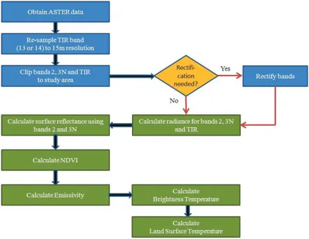
This tool was written in Visual Basic .NET and can be run on Microsoft Windows operating systems. There are five menus in the tool: 1- Radiance, 2- Reflectance, 3- NDVI, 4- Emissivity, and 5- Temperature. The flowchart of the program can be seen in Figure 1 below. At sensor Radiances for ASTER bands are computed from Equation 10 (Milder 2008; Ghulam 2009).

5

This tool was written in Visual Basic .NET and can be run on Microsoft Windows operating systems. There are five menus in the tool: 1- Radiance, 2- Reflectance, 3- NDVI, 4- Emissivity, and 5- Temperature. The flowchart of the program can be seen in Figure 1 below. At sensor Radiances for ASTER bands are computed from equation 10 (Ghulam 2009; Milder 2008).

𝐿𝐿𝐿𝐿𝑠𝑠𝑠𝑠𝑠𝑠𝑠𝑠𝑠𝑠𝑠𝑠= (𝐷𝐷𝐷𝐷𝐷𝐷𝐷𝐷 − 1) ∗ 𝑈𝑈𝑈𝑈𝑈𝑈𝑈𝑈𝑈𝑈𝑈𝑈 (10)

Figure 1- Flowchart for the program Şekil 1- Programın akış şeması

Where; Lsenis at sensor radiance, DN represents digital number, and UCC is unit conversion coefficient.

UCC values can be obtained from Table 4 below according to band’s gain setting. Furthermore, Figures 2 and

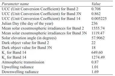
3 illustrate the radiance calculation interface of the software tool. Table 4- ASTER unit conversion coefficients (UCC) (Ghulam 2009) Çizelge 4- ASTER birim dönüştürme katsayıları (BDK) (Ghulam 2009)

ASTER UCC (W m-2_*sr*um)/DN)

Band High gain Normal Low gain 1 Low gain 2

1 0.676 1.688 2.25 NA 2 0.708 1.415 1.89 3N 0.423 0.862 1.15 3B 0.423 0.862 1.15 4 0.1087 0.2174 0.2900 0.2900 5 0.0348 0.0696 0.0925 0.4090 6 0.0313 0.0625 0.0830 0.390 7 0.0299 0.0597 0.0795 0.332 8 0.0209 0.0417 0.0556 0.245 9 0. 0159 0.0318 0.0424 0.265 10 NA 0.006822 NA NA 11 0.006780 12 0.006590 13 0.005693 14 0.005225 (10) Where; L_sen is at sensor radiance, DN represents digital number, and UCC is unit conversion coefficient. UCC values can be obtained from Table 4 below according to band’s gain setting. Furthermore, Figures 2 and 3 illustrate the radiance calculation interface of the software tool.

Figure 1- Flowchart for the program Şekil 1- Programın akış şeması

(6)

476

Ta r ı m B i l i m l e r i D e r g i s i – J o u r n a l o f A g r i c u l t u r a l S c i e n c e s 21 (2015) 471-482 Table 4- ASTER unit conversion coefficients (UCC)

(Ghulam 2009)

Çizelge 4- ASTER birim dönüştürme katsayıları (BDK) (Ghulam 2009)

ASTER UCC (W m-2_*sr*um)/DN)

Band High gain Normal Low gain 1 Low gain 2

1 0.676 1.688 2.25 NA 2 0.708 1.415 1.89 3N 0.423 0.862 1.15 3B 0.423 0.862 1.15 4 0.1087 0.2174 0.2900 0.2900 5 0.0348 0.0696 0.0925 0.4090 6 0.0313 0.0625 0.0830 0.390 7 0.0299 0.0597 0.0795 0.332 8 0.0209 0.0417 0.0556 0.245 9 0. 0159 0.0318 0.0424 0.265 10 NA 0.006822 NA NA 11 0.006780 12 0.006590 13 0.005693 14 0.005225

Figure 2- Radiance calculation interface for ASTER VNIR bands

Şekil 2- ASTER görünür yakın kızılötesi bantları için radyans hesaplama arayüzü

Figure 3- Radiance calculation interface for ASTER TIR bands

Şekil 3- ASTER termal bantları için radyans hesaplama arayüzü

After calculating at sensor radiances, planetary reflectances for ASTER bands (2 and 3N only) are computed using the Equation 11 (Ghulam 2009):

6

Figure 2- Radiance calculation interface for ASTER VNIR bands

Şekil 2- ASTER görünür yakın kızılötesi bantları için radyans hesaplama arayüzü

Figure 3- Radiance calculation interface for ASTER TIR bands Şekil 3- ASTER termal bantları için radyans hesaplama arayüzü

After calculating at sensor radiances, planetary reflectances for ASTER bands (2 and 3N only) are computed using the equation 11 (Ghulam 2009):

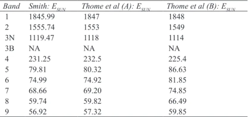
𝜌𝜌𝜌𝜌𝑇𝑇𝑇𝑇𝑇𝑇𝑇𝑇𝑇𝑇𝑇𝑇= (𝜋𝜋𝜋𝜋 ∗ 𝐿𝐿𝐿𝐿𝑠𝑠𝑠𝑠𝑠𝑠𝑠𝑠𝑠𝑠𝑠𝑠∗ 𝑑𝑑𝑑𝑑2⁄𝐸𝐸𝐸𝐸𝑆𝑆𝑆𝑆𝑆𝑆𝑆𝑆𝑆𝑆𝑆𝑆∗ cos (𝜃𝜃𝜃𝜃)) (11)

Where; 𝜌𝜌𝜌𝜌𝑇𝑇𝑇𝑇𝑇𝑇𝑇𝑇𝑇𝑇𝑇𝑇 is unitless planetary reflectance; Lsen is at sensor radiance; d is Earth-Sun distance in

astronomical units (populated from Table 5); ESUN is mean solar exoatmospheric irradiances (Table 6), and

𝜃𝜃𝜃𝜃represents solar zenith angle in degrees.

Table 5- Earth-sun distance (in astronomical units) (Ghulam 2009) Çizelge 5- Dünya-Güneş mesafesi (astronomik birim) (Ghulam 2009)

Earth-Sun distance in astronomical distance

DOY Distance DOY Distance DOY Distance DOY Distance DOY Distance

1 0.98331 74 0.99446 152 1.01403 227 1.01281 305 0.99253 15 0.98365 91 0.99926 166 1.01577 242 1.00969 319 0.98916 32 0.98536 106 1.00353 182 1.01667 258 1.00566 335 0.98608 46 0.98774 121 1.00756 196 1.01646 274 1.00119 349 0.98426 60 0.99084 135 1.01087 213 1.01497 288 0.99718 365 0.98333 (11) Where; is unitless planetary reflectance; Lsen is at sensor radiance; d is Earth-Sun distance in astronomical units (populated from Table 5); E_SUN is mean solar exoatmospheric irradiances (Table 6), and represents solar zenith angle in degrees.

Figure 4 shows the planetary reflectance calculation step of the program. This step requires four parameters: Julian Day, Mean Solar Exoatmospheric Irradiances, Solar Elevation Angle in Degrees, and Dark Object Value. Julian Day represents the day numbers based on acquisition date of the ASTER imagery. Mean Solar Exoatmospheric Irradiances can be obtained from Table 6 above and Solar Elevation angle is given in the header file. Dark Object value represents the area of zero reflectance below the pixel with the lowest reflectance values in the image. NDVI values can be computed easily after planetary reflectance values are calculated for ASTER bands 2 and 3 as illustrated in Figure 5 below. Afterwards, this NDVI file is used as an input to calculate emissivity values shown in Figure 6. The brightness temperature calculation step requires K1 and K2 radiation constants, which can be