TOBB UNIVERSITY OF ECONOMICS AND TECHNOLOGY INSTITUTE OF NATURAL AND APPLIED SCIENCES
COMPETITIVE INTERMODAL HUB LOCATION MODEL WITH
ENDOGENOUS PRICING
M.Sc. THESIS
M. Reza MOUSAVI ALMALEKI
Department of Industrial Engineering
Approval of the Graduate School of Science and Technology.
………..
Prof. Dr. Osman EROĞUL
Director
I certify that this thesis satisfies all the requirements as a thesis for the degree of Master of Science.
……….
Prof. Dr. Tahir HANALIOĞLU
Head of Department
The thesis with the title of “Competitive Intermodal Hub Location Model with
Endogenous Pricing” prepared by M. Reza MOUSAVI ALMALEKI M.Sc.
student of Natural and Applied Sciences institute of TOBB ETU with the student ID 161311055 has been approved on 10.12.2019 by the following examining committee members, after fulfillment of requirements specified by academic regulations.
Thesis Advisor: Assist. Prof. Dr. Salih TEKIN ...
TOBB University of Economics and Technology
Thesis Co-advisor: Assist. Prof. Dr. Gültekin KUYZU ...
TOBB University of Economics and Technology
Examining Committee Members:
Assoc. Prof. Dr. Babek ERDEBILLI (Chair) ... Yildirim Beyazit University
Assoc. Prof. Dr. Kürşad DERINKUYU ...
THESIS STATEMENT
Tez içindeki bütün bilgilerin etik davranış ve akademik kurallar çerçevesinde elde edilerek sunulduğunu, alıntı yapılan kaynaklara eksiksiz atıf yapıldığını, referansların tam olarak belirtildiğini ve ayrıca bu tezin TOBB ETÜ Fen Bilimleri Enstitüsü tez yazım kurallarına uygun olarak hazırlandığını bildiririm.
I hereby declare that all the information provided in this thesis was obtained with rules of ethical and academic conduct. I also declare that I have sited all sources used in this document, which is written according to the thesis format of Institute of Natural and Applied Sciences of TOBB ETU.
M. Reza MOUSAVI ALMALEKI
ABSTRACT
Master of Science
COMPETITIVE INTERMODAL HUB LOCATION MODEL WITH ENDOGENOUS PRICING
M. Reza MOUSAVI ALMALEKI
TOBB University of Economics and Technology Institute of Natural and Applied Sciences Department of Industrial Engineering
Advisor: Assist. Prof. Dr. Salih Tekin Co-advisor: Assist. Prof. Dr. Gültekin Kuyzu
Date: December 2019
Road transportation has successively captured the majority of the transportation market in most of the economies. Massive amounts of flows are moving through road network, which is resulting in an unsustainable economy with congestion and environmental problems. In order to tackle the problem, intermodality can be utilized in logistics networks. Railroad transportation is one of the smooth ways of transportation in several ways. It can reduce the congestion and also it is more cost effective. In order to be able to utilize the economy of scale and reduce the transportation cost in the logistics network, hubs can be established in some points of the network. Understanding the transition of demand under a competitive intermodal hub location model is the aim of this study. One of the most important factors in customer behavior is the price that the firm is charging and it is more reasonable to model the demand as a function of price. To do so, a discrete choice logit model is applied in a Mixed Integer Nonlinear Programming (MINLP) framework and an efficient heuristics solution is provided. Moreover, actual Turkish network data for rail transport is being considered in the model, on top of the CAB data and optimal price strategy is derived out of the model.
Keywords: Intermodal competition, Freight transportation planning, Hub location,
Discrete choice, Pricing.
ÖZET
Yüksek Lisans Tezi
İçsel Fiyatlandırma Tabanlı Rekabetçi Intermodal Dağıtım Merkezi Belirleme Modeli M. Reza MOUSAVI ALMALEKI
TOBB Ekonomi ve Teknoloji Üniveritesi Fen Bilimleri Enstitüsü
Endüstri Mühendisliği Anabilim Dalı
Danışman: Yrd. Doç. Dr. Salih Tekin Eş Danışman: Yrd. Doç. Dr. Gültekin Kuyzu
Tarih: Aralık 2019
Karayolu taşımacılığı, taşımacılık pazarını başarılı bir şekilde yakalamış durumdadır. Büyük miktardaki yük akışı karayolu ağı üzerinden sağlanmaktadır. Büyük miktalardaki yük akışı tıkanıklık ve çevre sorunları ile sürdürülemez bir ekonomiyle sonuçlanamaktadır. Daha sürdürülebilir bir çevre sağlamaya yönelik olarak lojistik ağları modalite yöntemi çerçevesinde planlama yapılabilmektedir. Tren taşımacılığı bazı nedenlerden ötürü pürüzsüz bir taşımacılık hizmeti sunmaktadır. Sıkışıklığı azaltabilir ve aynı zamanda daha uygun maliyetlidir. Lojistik sektöründeki ölçek ekonomisini kullanabilmek ve nakliye maliyetini düşürebilmek için, yük taşıma ağının bazı noktalarında dağıtım merkezleri kurulabilir. Bu çalışmada, geliştirilen rekabetçi intermodal merkez lokasyon modeli altında talep dinamiğin incelenmesi amaçlanmıştır. Müşteri davranışında en önemli faktörlerden biri firmanın uyguladığı fiyat politikasıdır. Bu bağlamda, talebin bir fiyat fonksiyonu olarak modellenmesi daha makul bir yaklaşım sunmaktadır. Buna yöneli olarak, bu çalışmada ayrık seçim logit modeli uygulanmaktadır. Ayrıca, demiryolu taşımacılığı için gerçek veriler modelde dikkate alınmakta ve Karışık Tamsayı Doğrusal Olmayan Programlama (KTDOP) modelinden optimal fiyat stratejisi elde edilmektedir ve etkin sezgisel çözüm verilmiştir.
Anahtar Kelimeler: İntermodal yarışma, Yük taşımacılığı planlaması, Dağıtım
ACKNOWLEDGEMENT
Many thanks for help and support to Dr. Salih Tekin and Dr. Gültekin Kuyzu who guided the procedure of the study with their valuable comments and feedback and great acknowledgment for TOBB ETU due to its scholarships and support. Special thanks to my family and all friends who made enjoyable moments.
CONTENTS Page ABSTRACT………...iv ÖZET………v ACKNOWLEDGEMENT………....vi CONTENTS………...vii LIST OF FIGURES………...viii LIST OF TABLES………...ix 1. INTRODUCTION ... 1 1.1 Literature Review ... 2 1.1.1 Intermodality... 2 1.1.2 Hub location ... 3
1.1.3 Demand and price changes ... 4
2. PROBLEM DEFINITION ... 7
2.1 Mathematical Model...10
3. SOLUTION APPROACH ... 15
3.1 Convexity and Concavity Discussion ... 15
3.2 Two Stage Solution ... 18
3.2.1 Strategic optimization ... 19
3.2.2 Operational optimization ... 21
3.3 Heuristics ... 22
4. COMPUTATIONAL EXPERIMENTS ... 25
4.1 Data and Parameters ... 25
4.2 Results ... 26
4.2.1 CAB data results... 28
4.2.2 Turkish network solutions ... 30
4.3 Scenario Analysis ... 34
5. CONCLUSION ... 39
REFERENCES………...41
APPENDIX………...45
LIST OF FIGURES
Page
Figure 1.1: Intermodal terminals for European countries...1
Figure 1.2: Unit energy consumption for load transportation...2
Figure 2.1: Topology of nodes in the model ... ..9
Figure 2.2: Available routes ... 10
Figure 4.1: Profit and market share levels of rivals with respect to price ... 29
LIST OF TABLES
Page
Table 4.1: Objective function values for different models and solutions... 27
Table 4.2: 25-node CAB data network solutions with α=0.07 ... 29
Table 4.3: 25-node CAB data network solutions with α=0.07 and θ=0.0035 ... 30
Table 4.4: 81-node Turkish data network solutions with p=10 and θ=0.004 ... 32
Table 4.5: 81-node Turkish data network solutions with α=0.7 and p=10 ... 32
Table 4.6: Comparison of two scenarios for entrant, α=0.7, γ=0.6 and θ=0.004 ... 35
Table 4.7: Entrant’s profit and market share with respect to its price, α=0.7 and θ=0.004 ... 36
Table 4.8: Comparison of price for the incumbent and entrant for two origin destination cities when α=0.3 and θ=0.01... 37
1. INTRODUCTION
Freight transportation is an essential part of the economy for countries to link the de-mand and supply sides to each other by shipment of raw materials, goods and final products. Economic limitations motivate the industries and agents to seek smoother and more cost effective ways for their supply chain management in order to increase the performance. Freight transportation networks experience different trends as new industries are growing and also customers need more efficient services. This would require shippers and cargo service providers to operate in a lower cost by keeping their quality increased. Furthermore, new managerial strategies and insights are needed to achieve a more sustainable and efficient transportation system since it contributes to a large share of the cost in the supply chain [15].
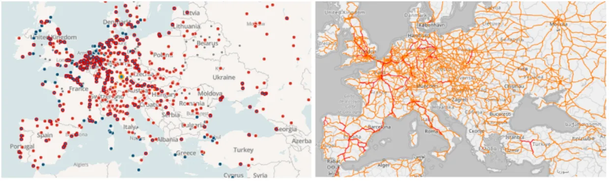
Road transportation has successively captured the transportation market. Massive amo-unts of flows are moving through the road network, which is resulting in an unsusta-inable economy with congestion and environmental problems. It is responsible for a considerable share of energy among different energy sectors and also causes climate degradation. As a case for Turkey, transportation is the second sector in energy sumption which contributes to 24% of total energy consumption and 98% of this con-sumption is supplied by petroleum and only 2% by natural gas [1, 40]. Moreover, 91% of load transportation is carried out by trucks and road freight and only 6% allocates to rail shipment [2]; as it can be seen in the Figure 1.1, the rail traffic and intermodal terminals for Turkey are scarce with respect to other developed European countries.
Figure 1.1: Intermodal terminals for European countries.
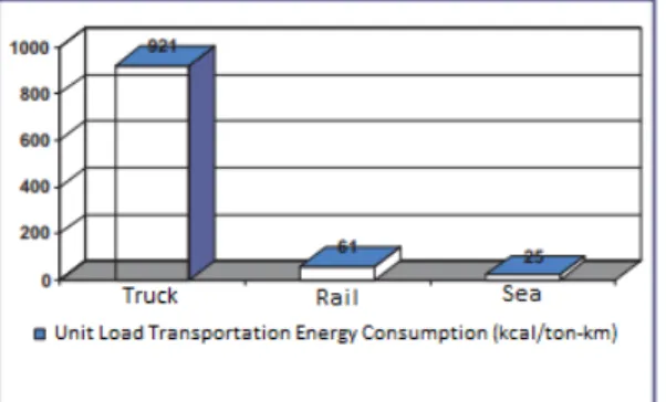
This occurs while the energy consumption of rail sector is clearly less than road sector as shown in Figure 1.2. Unless other energy consuming sectors, e.g. industry,
electri-city, household and residential, carbon emission is not remedied during the past years. Thus, popularity of other transport modes would improve the logistic system environ-mentally in a way that less energy would be consumed; it is also profitable for these sectors to participate more in the market.
Figure 1.2: Unit energy consumption for load transportation
1.1 Literature Review
In order to achieve a more sustainable economy and solve the problems that the road transportation brings, intermodality can be planned in logistics networks [21]. Inter-modal network refers to a transportation system in which freights are moved via more than one transportation mode from origin to destinations through a smooth manner by using terminal nodes and intermodal cargo containers [24, 38].
European Commission is developing and supporting intermodality to promote other transportation modes, rather than road, so that its advantages would improve the eco-nomy and environment. In an intermodal framework, majority of the transportation is done by rail, sea or other environmental friendly modes, while shorter routes may be capture loads by road. Marco polo program is planned by the commission in order to shift freight transportation from trucks and road to other modes; 2018 was named the year of multimodality by EU transport commissioner. Intermodal shipment is also increasing in the US domestic freight movement [18].
1.1.1 Intermodality
Utilizing integrated intermodal service for shipment of cargo from origin to destination in the logistics network is both tactically and operationally efficient not only because of the cost reduction opportunities but also due to the higher capabilities of the inter-modal service [33]. The capability of the network would increase by larger capacity,
volume and operational availability in the intermodal shipment, while most of the road freight transportation attribute to lower capacity and volume, higher operational time due to the increased number of trucks, managerial difficulties and shortages in capabi-lities. These issues can be taken care of by usage of rail transportation in the network since it can handle more capacity, volume and weight compared to the road service. It may be noticed that there might be access issues while transferring goods via rail network due to possible lack of stations and terminals in a specific region. This would overcome by help of road service to pick up the freight from the origin and deliver it to the destination, while the majority of the transportation would be carried out via intermodal shipment. It is worth noticing that although intermodality is subjected to a competition between road and the intermodal service firms, cooperation of these two actors is also possible, since dead heading would be addressed as a result of coalition between road and intermodal freight service.
Railroad transportation is one of the smooth ways of transportation in several ways. It has more capacity and hence, will reduce the number of its road competitors in the fi-eld. It can reduce the congestion and also it is more cost effective. Energy consumption is also less in rail sector.
1.1.2 Hub location
In order to be able to utilize the economy of scale and reduce the transportation cost in the logistics network, hubs can be established in some points of the network. Hub -spoke environment is widely used in the literature since the famous paper of O’Kelly [27] and provide a good framework for analyzing the flow transition in a network. Se-lecting some nodes among a number of existing nodes in a network as hub cities is considered as hub location problem. Hub location problem is one of the prosperous research fields that is being used in several different areas not only in transportation and logistics, but also in computer science [3]. Telecommunication is one of the main areas that started using hubs, later, it has been applied to many different fields like marine industry, message delivery networks, post firms on top of the logistics and different transportation systems. Hubs are reducing the number of possible routes bet-ween origin destination pairs. Inserting only one hub to a fully connected network with size k would reduce the number of routes needed to connect all demand pairs by (k-1)(k-2) without connecting non hubs nodes or spokes [14]. Hence, more efficient and cost-effective network transportation would be planned by exploiting hubs rather than having a fully connected network. Demand and flow are assumed to be moved from
origin to destination cities through selected hubs and these hubs would implement con-solidation effect inside the network. As a result of these concon-solidations, the network would utilize economy of scale at inter-hub transport, which yields to lower cost and more efficient plan for the flow of the demand between nodes and origin-destination targets.
Hub location problem can be seen from different points of view. Evaluating the ca-pacity of the network or arcs is one measure that the problem can contain. Moreover, allocating nodes such that each node is linked with only one hub, forms single alloca-tion problem types, and on the other hand, if each of origin- destinaalloca-tion pairs can be connected to more than one hub, the problem is multiple allocation hub location. La-tely, approaches toward considering different types of transportation modes, demand and price uncertainty, time and congestion and queuing have become popular in the literature. Several hub location problems review can be found at the following articles [3, 8, 14, 19].
Different aspects have been considered in hub location problems. Recent trends inc-lude solving the problem more efficiently in shorter time with larger problem size. Polyhedral tools are used in some applications [17], along side with new algorithms and techniques for solving network design of the facility location problem, more com-pact solutions are provided in some works [23]. Methods like Benders Decomposition used in more recent studies [12, 30].
1.1.3 Demand and price changes
When a new transportation mode is entering to the market, by establishing hubs, it is important to notice that demand of customer would not stay unchanged [34]. The level of service that the entrant firm is providing can determine the customer behavior. Inter hub scale effect is considered as the most important reason for utilizing hubs at the logistics network [20]. In a proper modelling framework, the amount of load transmitted through hub and spoke should be large enough so that a discount cost could be applied on the service level of the intermodal company, however, in some cases the traffic may be so small that the economy of scale is not reasonable to be applied on the network [11, 29]. The basic hub location problem assumes a fully interconnected network, i.e. all hubs are connected to each other, in which a discount parameter (α) is applied on the inter hub route transportation cost. This scale assumed to be fixed and independent of the flow or demand volume at the route, also it does not consider the traffic of the route and discounted arcs would operate among the interconnected routes
between hubs. Although most of the works are considering the flow independent fix discount factor (α) due to its convenience, incorporating the economy of scale into the the hub location problems is under study and generally there are specific ways to do so. Firstly, approximating the non-linear function of the discount between hubs via a piece-wise linear function is considered [20, 29]. Other studies utilize incomplete networks [4, 10] and thirdly, hub-arc models are addressing the discount in the hub location problems [7, 7]. Some other studies allocate a certain amount of flow to the inter hub routes [31].
The price that the intermodal firm charges is one of the most important factors in cus-tomer behavior at networks [22]. Spatial price equilibrium in networks is evaluated by several important and pioneer studies [32]. The literature is scarce on the intermodal problem with endogenous demand and price. Elastic demand with an equilibrium of economic conditions is provided in some studies [30]. There are studies that state that there is no study on pricing in intermodal framework [14, 19]. Villagra and Marianov analyze a competitive hub location problem where leader and follower would decide on opening hubs as a result of competition and use metaheuristics to solve the nonli-near model [22]. Very few examples in the literature can be mentioned where the prices of intermodal services are tackled as decision variables through a mathematical prog-ram. In a different approach, Zhang et al. develop a framework to evaluate intermodal port competition of two ports in China with game theory [45]. They suggest that not necessarily increasing the number of ports would result in more market share for inter-modal firm. In an intercity framework, Gremm analyzes the competition of railway and bus services with a regression model and conclude that intermodal prices are less than monopolistic routes prices [16]. Zhang et al. develop a theoretical model without ope-rational considerations to obtain optimal price for an intermodal competition with road sector by basing the decision model on minimum logistic costs [39]. With more focus on revenue management, Riessen et al. considered a transportation of marine shipment by allowing different fare classes [41]. They extend the work on intermodality and conclude that this class can have a remarkable effect on the revenue management [42]. Wang also noticed the fare class in the revenue management of an intermodal network with considering the two important levels of analyzing, tactical and operational, by developing a mixed integer model [43]. A review of pricing problems in intermodal context is provided at Tawfik and Limbourg’s review paper [37].
It can be seen that most of the studies in the hub location problem environment are focusing on minimizing the cost of the network, however, analyzing the demand side and finding an efficient pricing strategy for the firm that operates hub in its network is
one of the interesting and important issues.
The key question that motivates the study is the existence and amount of profit that the intermodal company can achieve in competition with the incumbent. Under which conditions the intermodal corporate would be better off? how many hubs should be selected and where should be operating? what should be the structure of routes and connections? Also, an important question is what is the efficient pricing strategy for the intermodal company. What is the price that contributes to the optimal profit and does it accompany with the market assumptions?
To the best of authors knowledge, there is no work that model the competitive intermo-dal hub location problem with endogenous demand that is being captured by discrete logit model as a function of price and solved by two stage approach. This frame work is more reasonable in modeling the flow transitions after entering the new firm to the market.
The contributions of this study are many fold. Firstly, a unique intermodal two stage problem is developed so that strategic and tactical/operational decisions would be eva-luated in order to consider competition of intermodal company with road freight ship-ment with considering the relation of demand, market share and optimal pricing st-rategy. Secondly, a discrete choice non-linear model is characterized to formulate the dynamics of price and market share. Also, an efficient solution method is provided for solving the non-linear problem without prevalent computational inconvenience. Imp-lementing actual Rail data into the model and specifying network features for real topology of road- rail is another attainment. Complete sensitivity analysis is carried out and conditions in which intermodal shipment would gain more profits than road cargo is stated. Understanding the transition of demand under a competitive environ-ment would be aim of our study.
The rest of the study is organised as follows. Model environment and frame work is described in the next section where the model formulation of two stages of strategic and operational is provided afterward. Solution and results are showed in the next section and final remarks are expressed finally.
2. PROBLEM DEFINITION
In this thesis, an intermodal problem is addressed in which the incumbent, road ship-ments, is already in the market and operating through its fully connected network wit-hout establishing or using hubs in its topology and its revenue comes from charging a specified yield over the cost for the customer.
The competition environment is captured by entering the new intermodal company, which is rail, to the same market and its attempt to gain the market demand shares from the road company and increase its own share of the market by applying certain strategies, i.e. establishing and employing its facilities in the network as hubs, usage of the routes and determining an efficient pricing strategy by evaluating the demand and market share that is being earned for the intermodal company. The company has its own network, with hubs and spokes, while it would use roads for out-hub trans-portation. The inner-hubs shipment is carried out by the intermodal company. It will be analyzed whether the intermodal company would rather to put the priority on more market share over price or not. The problem would aim to maximize the profit and provide an efficient pricing strategy, on top of a cost effective hub and spoke network topology. The customer decides on selecting the shipment company based on the costs and price of the both companies and a discrete choice logit model would capture the customer’s behavior in the model.
Discrete choice logit model is widely used after early works of Berkson [5] in different subjects, afterward, McFadden et al. addressed the discrete choice logit model in travel behavior context [25].
The logit choice probability model is popular because of its convenience to form a close form for different choice probabilities of a set and also it provides a framework that the estimated probability that underlies between zero and one [28]. Moreover, it provides a useful framework so that different variables or parameters and their effects on the model can be analyzed through the probability choice model. Ortuzar et al. suggest that the logit model can be used justifiably in the transportation and freight shipment literature to evaluate the probability choice of different issues in the problem [13]. the model is used in this study to examine the relationship between market share and pricing strategy of the intermodal company in a way that price and market share
play a counter role with respect to each other. It is beneficial for the logit model that enables the model to simulate the problem more rationally, since the intermodal com-pany cannot always increase its price wishing to obtain higher profit saying that the price is present at the maximizing objective function.
Despite its advantages, logit model is the source of non-linearity in the model. The incumbent is taken as the base in the denominator and the intermodal pricing at the nominator. The solution approaches are discussed further in the study.
General assumptions of the hub location problems are often considered as the follo-wings:
• All hub nodes are assumed to be connected and interconnection of hub nodes is satisfied by existence of a link between each hub pair.
• Presence of inter-hub discount that is attributing economies of scale by setting a discount factor into the links between hub pairs which is due to availability of higher capacity, volume, weight and energy consumption saving.
• Origin destination nodes cannot be linked without being connected to hubs, which means that direct service is not allowed for non-hub nodes.
However, in this study the assumptions are slightly different and an existing road trans-portation network would compete with intermodal rail logistics in the supply chain under the succeeding conditions:
• First of all, the network is fully connected for the road company which is ope-rating currently at the field and all supply-demand points are connected by the existing routes.
• Road service is operating direct links through each origin destination pairs wit-hout usage of hubs or terminals and all market share is being captured by this direct strategy of the road freight service.
• With regard the pricing strategy, road is exhibiting a lump sum pricing strategy by which it charges a certain amount of profit with respect to the direct route cost.
• Rail shipment, on the other hand, would enter to the market by utilizing hub location and routing problem at the strategic level and then by developing an operational level of decision making through efficient pricing bundle.
• Rail stations are already operating in the network and there is no fixed cost of establishing a new facility for the railroad company.
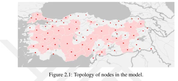
Due to the lack of managerial cooperation Railroad does not employ hubs and routing problem and operates like the existing road freight service by usage of direct links. Figure 2.1 shows the nodes that are included in to the model, dots are representing road nodes and railroad is operating at the stations that are active in colored regions.
Figure 2.1: Topology of nodes in the model.
The model provides a framework to consider the effect of utilizing intermodal hub and spoke routing network and asses the revenue management of the rail shipment. To do so, the model framework would assume that:
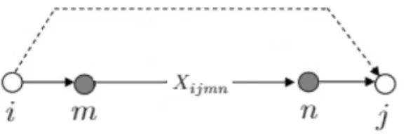
• Railroad company would specify some nodes as hubs and carries out rail trans-portation between hubs as Figure 2.2 shows.
• Maximum number of hubs for each origin destination route is two and origin to hub and hub to destination delivery is being done by truck.
• There is no full interconnection between hubs.
• Routing of freight flows does not make congestion in hubs or its levels are assu-med to be negligible.
• Goods are also assumed to be homogeneous and different types of goods wo-uld not effect the freight shipment and standard cargo containers are carried out through the network.
• Transportation cost is the main source of cost in the network and since the in-termodal company already has its own network and stations with facilities, no establishment cost or fixed cost is contributed.
• The road company does not utilizes hubs, while rail transportation would use maximum of 2 cities as hubs in the route.
Figure 2.2: Available routes.
Uncapacitated facility location and routing problem would be evaluated and intermodal company would apply a discount factor on the inter hub connections that is independent of the load volume and does not depend on the traffic of the route. This scale effect is the motivation for the intermodel company to compete with the road transmits. The problem aims to maximize the profit of the intermodal company, i.e. rail, by specifying an optimal pricing strategy where certain freight market share would be allocated to the rail company.
The inter-hub transportation is being done by rail and out of hub transportation, which is generally consists of small distances, is carried out by normal road trucks but through the intermodal company, since the main shipment is between hubs and is executed by the intermodal company.
2.1 Mathematical Model
The initial model for addressing the problem is developed.
Parameters:
• Wi j: The total amount of flow or demand transported from origin city i to
desti-nation city j.
• p: Number of hubs to be allocated. • Crail
i jmn, Ci jroad: Distance cost for rail and road company, respectively.
• drail
mn : Distance between city m and n in the rail network.
• droad
i j : Distance between city i and j in the road network.
• α: Service level of rail company, or scale effect of hubs. • ∆: Profit percentage
• Θ: Consumer sensitivity to the price. Variables:
• hm: Binary variable which is 1, if city m is assigned to be a hub, and 0 otherwise.
• Xi jmn: Binary variable which is 1, if rail company uses a route for origin
destina-tion cities i and j through hubs m and n, and 0 otherwise. • Prail
i jmn: Positive variable, the price that rail company charges for the origin
desti-nation cities i and j using cities m and n as hubs. • Lograil
i jmn: Fraction of demand for origin destination cities i and j that rail company
captures by using hubs m and n.
• Logroadi j : Fraction of demand for origin destination cities i and j that road com-pany captures after entering the rail comcom-pany to the market.
The mixed integer non-linear problem (MINLP-Logit Model) is described as the following:
Max
∑
i∈Nj∈N
∑
m∈K∑
n∈K∑
(Pi jmnrail −Ci jmnrail )(Wi j)(Lograili jmn) (2.1)
Subject to:
∑
m∈K hm= p, (2.2)∑
m∈Kn∈K∑
Xi jmn≤ 1, ∀i, j ∈ N, i 6= j (2.3) Xi jmn≤ hm, ∀i, j ∈ N, i 6= j & ∀m, n ∈ K, m 6= n (2.4) Xi jmn≤ hn, ∀i, j ∈ N, i 6= j & ∀m, n ∈ K, m 6= n (2.5) (∑
m∈Kn∈K∑
Lograili jmn= Xi jmnhmhnexp(−ΘP
rail i jmn)
∑s∈K∑t∈KXi jsthshtexp(−ΘPi jstrail) + exp(−ΘPi jroad)
, (2.7) (∀i, j ∈ N, i 6= j&∀m, n ∈ K, m 6= n&s < t)
Ci jmnrail = (dimroad+ αdmnrail+ dn jroad)Xi jmn, ∀i, j ∈ N, i 6= j & ∀m, n ∈ K, m 6= n (2.8)
Pi jroad = (1 + ∆)di jroad, ∀i, j ∈ N, i 6= j (2.9)
Ci jmnrail −Ci jroad ≤ (1 − Xi jmn)M, ∀i, j ∈ N, i 6= j & ∀m, n ∈ K, m 6= n (2.10)
Ci jroad= di jroad, ∀i, j ∈ N, i 6= j (2.11)
Xi jmn∈ {0, 1}, ∀i, j ∈ N, i 6= j & ∀m, n ∈ K, m 6= n (2.12)
hm∈ {0, 1}, ∀m ∈ K (2.13)
0 ≤ Lograili jmn, Logroadi j ≤ 1, ∀i, j ∈ N, i 6= j & ∀m, n ∈ K, m 6= n (2.14)
Pi jmnrail ≥ 0, ∀i, j ∈ N, i 6= j & ∀m, n ∈ K, m 6= n (2.15)
It can be noticed that the objective function (2.1) is non-linear due to presence of price and market share. The objective is maximizing the total profit of the intermodal
company, rail transportation, by calculating the revenue and cost for each route and accumulate for the net profit. The first four constraints (2.2-2.5) are usual constraints in the p-hub models that ensure existence of p hubs in the network with a unique route that passes through hubs for each origin-destination pair, if existed. Constraints (2.6) and (2.7) are essential for the model and are the discrete choice logit model as the share of the market that rail and road firms can allocate to their OD route. For each route, the share of demand that both companies can afford to carry must sum up to one and for the rail company it would be determined by the non-linear constraint (2.7) which is the logit share of the rail shipment that has an inverse relation with the price that is charged for the specific route. Unlike the all-or-nothing strategy, this constraint enables the model to consider a proportion of the flow that can be allocated to the intermodal sector. Cost structure of the network is given by constraints (2.8) and (2.11). The scale effect is incorporated for the intermodal service as the inner-hub transportation is assumed to have a significant discount over the normal truck shipments that have the distance as a representative of the transportation cost. The pricing strategy of the road sector is provided in constraint (2.9), that assumes that a certain profit rate would be exerted on the cost for the road service. On a geometric basis, it is logical to assume that the intermodal service would establish a connection route between any OD pair in which its cost is less than the road sector’s cost. This fact is captured in constraint (2.10). Constraints (2.12-2.15) explain the domain of the variables in which X and h are binary variables, while price and market shares are positive with natural bound for the flow proportions that should lie between zero and one as they are probabilities.
3. SOLUTION APPROACHES
Considering the mentioned plan, the problem is solved by GAMS-BARON and Java-Eclipse. Optimal objective function for rail firm should be calculated for different pa-rameters. Furthermore, optimal price for each route needs to be computed by solving the discrete choice model. It is easy to notice that the model is significantly exhaus-tive for computation due to non-linear formulation and existence of 4 index variables. However, considering the price and the market share as the two important positive va-riables of the model, convexity analysis can be performed by relaxing the domain of the analysis into the nodes that binaries are established to be one. By doing so, for each OD route, a continuous and differentiable logit function can be evaluated. The intuition comes from studies in the intermodal pricing literature that suggest that the problem can be viewed from two points of view. A strategic profit maximization problem can be solved in the first place and then operational and reactions of the customer can be considered in a lower level in order to solve the pricing problem of the intermodal ser-vices [36]. This approach, bilevel optimization problems, introduced by Bracken and McGill [6], provides a useful method to handle the Stackelberg games and has a wide usage in transportation problems where the incumbent and entrant seek to optimize their utilities and make a more efficient network [9]; and also one advantage of this approach is taking into account the strategic decisions that affect the problem at the first place. Similar studies benefit from this framework, for example, in a multimodal network, Yamada et al. provide a bilevel optimization with a discrete network design in the upper level and the traffic assignment in the lower level [44]. Although technical bilevel structure is not used in this study, geometrical and strategic decisions regarding the network designs is implemented in the first stage and then operational decisions about price and market shares is calculated in the second stage. Hence, a two stage problem solving method is developed in order to solve the problem.
3.1 Convexity and Concavity Discussion
Convexity of the logit constraint is important in problem solving of the mentioned model and literature review shows that rare studies can be found that address the logit model’s convexity in this context.
The discrete choice logit model is roughly a function of intermodal price and also bi-nary location and route variables. By relaxing the integrity property of the bibi-nary vari-ables it can be said that the logit constraint (2.7) is a continuous and twice differentiable function of the three mentioned variables. It is defined for each route i − m − n − j, for the route’s intermodal price (Pi jmnrail) and binary variables (Xi jmn, hm, hn). For the
simpli-city the function Lograili jmn(Pi jmnrail, xi jmn, hm) is considered as Log(P, x, h) and its Hessian
matrix is calculated as follow:
H= ∂2Log ∂ P2 ∂2Log ∂ P∂ x ∂2Log ∂ P∂ h ∂2Log ∂ x∂ P ∂2Log ∂ x2 ∂2Log ∂ x∂ h ∂2Log ∂ h∂ P ∂2Log ∂ h∂ x ∂2Log ∂ h2
The derivatives are available at the Appendix section. We know that a matrix H is positive semi definite if and only if the determinant of each square matrix is non-negative.
Definition: For a symmetric matrix H, a principal minor is the determinant of a sub-matrix of H which is formed by removing some rows and the corresponding columns. Theorem: For a symmetric matrix H, if all principal minors of H are nonnegative, then the matrix is positive semi definite .
Proof: We prove the contra-positive by induction. We may assume that H has a unit eigenvector v with eigenvalue λ < 0. If H has only one eigenvalue which is not posi-tive, then det(H) < 0 and the relation holds. Otherwise, choose a unit eigenvector u orthogonal to v with eigenvalue µ which is not positive. Now, choose s ∈ R so that the vector w = v + su has at least one zero coordinate, say the ith. If H0 is the matrix obtained from H by removing the ithcolumn and row and w0is obtained by removing the ithcoordinate of w, then we have (w0)TH0w0= wTHw= λ + s2µ < 0. So, H0is not semidefinite, and the result follows by applying induction to it.
Hence, starting with the h31element of the Hessian matrix the first condition is satisfied
since ∂2Log
∂ h∂ P is non-negative. Next, the second determinant is calculated as h21h32−
h22h31 and if we impose the non-negativity condition the below expression is obtained:
(2hmXi jmnA3)exp(−ΘPi jmnrail) ≥ B2 (3.1)
WhereA= Xi jmnhmexp(−ΘPi jmnrail) + exp(−ΘPi jroad)andB= Xi jmnhmexp(−ΘPi jmnrail) − exp(−ΘPi jroad).
Inequality (3.1) is the necessary but not sufficient condition for the convexity of the 16
logit constraint. The inequality is not satisfied if either of X or h is equal to zero. In the case that both of them are equal to one, the expression would reduce to:
2exp(−ΘPi jmnrail)[exp(−ΘPi jmnrail) +C]3≥ [exp(−ΘPi jmnrail) −C]2 (3.2) Where C= exp(−ΘProad
i j ). The last determinant that should be examined is the detH.
Again, if either of the X or h variables is zero the determinant is negative. If both of them are equal to one, the positive determinant is achievable if:
2[exp(−ΘPi jmnrail)]2[1 +A
3
B2− 2A
2] + 1 ≥ 0 (3.3)
In summary, for a specific i − m − n − j route, the Hessian matrix is positive semi definite; so the logit constraint is convex; if both hmand Xi jmnare equal to one and (3.2)
and (3.3) inequalities are satisfied. Convexity of the logit constraint is not guaranteed if either of the location decision variables is zero. This is another motivation to divide the problem into two levels, since the analysis shows that the market share and pricing strategy can be optimised under the condition that location variables are determined. Now we assume that location variables are known and the logit constraint (2.7) is considered for those of them who are equal to one. Once the location problem is solved, the constraint (2.7) is a continuous and twice differentiable function of intermodal price and convexity of the logit function can be evaluated under less restrictive conditions. Knowing the values of location decision variables, the logit function is reduced to:
Log(Prail|X, h) =
ˆ
X ˆhexp(−ΘPi jmnrail) ˆ
X ˆh ∑s∈K∑t∈Kexp(−ΘPi jstrail) + exp(−ΘPi jroad)
,
and by imposing the non-negativity condition on the second derivative of the logit function with respect to intermodal price, the below condition is achieved:
Pi jroad ≤
∑
s∈Kt∈K
∑
Pi jstrail (3.4)
So, given the location decision variables, Inequality (3.4) shows the condition under which the logit constraint (2.7) is convex, that suggests that the optimization model would prefer to attain higher prices for the intermodal company compare to the road shipment for a given route that include hubs.
To discuss the concavity of the objective function under the assumption of given loca-tion variables, as a maximizing problem is solved, it can be noticed that the objective (2.1) consists of two terms. The second term, associated with cost, is concave; since it is a negative of a convex function given the condition (3.4). For the first term of the objective, we need to calculate the second order derivative of G(Prail) = W PrailLograil with respect to intermodal price. Non-positive second derivative of the G is obtained if: Prail− Proad≤ 1 θ ln( θ Prail+ 2 θ Prail− 2); (θ P rail> 2) (3.5)
The concavity of the objective function is attained by conditions (3.4) and (3.5), gi-ven the location decision variables. These two expressions provide a range in which the intermodal price can move so that the logit constraint is convex and the objective function is concave, when the location variables are given.
The convexity analysis shed light on the possible technique to solve the presented mi-xed integer nonlinear problem (MINLP). Based on the previously mentioned reasons, defining two stages of the decision making enables us to solve the problem more effici-ently without loosing comprehensive information or available solutions. It is worth no-ticing that, if conditions (3.4) and (3.5) are satisfied, then the conditions (3.2) and (3.3) are also satisfied, which means that convexity of the logit model when the location variables are known (as established hubs and routes), has the same implementations with the case that they are not known. Hence, at the end of the analysis in both cases, the problem is evaluated when the location variables are equal to one. This shows the equivalence of examining the model with two strategic and operational stages with a single mathematical model, since in both settings, the hierarchy can be noticed that by finding the location variables first, we can tackle the operation level and determine the logit market share with its associated intermodal price.
The convexity conditions are suggesting that the intermodal prices should be higher than incumbent’s prices, as conditions (3.4) and (3.5) show, but this does not mean that the optimal prices would be higher than road’s prices necessarily. Later in the solution part, it will be shown that there are routes in which the optimal intermodal price is less than incumbent’s price.
3.2 Two Stage Solution
In the literature of intermodal price studies, there are few works which address both strategic and operational levels. [41] model a marine container transportation problem with focus on its revenue increase by defining two decision making levels. At the tacti-cal level, fare settlements and limits are tacti-calculated and price considerations are handled at the operational level. [43] also developed a mixed integer linear program at both two levels to evaluate the revenue and price for barge transportation network.
This study examines the both decision making level by modeling both levels clearly in order to solve the intermodal pricing problem. As so, to find the optimal pricing portfolio for the rail company, a two stage optimization model is developed. Stages of decision making in the problem are divided into two levels, firstly, a strategic decision would be made on the hubs and connectivity of the cities, and then an operational plan would specify the prices and market share of the service that rail company provides. For the strategic stage, firm would decide which cities to use as hubs. Since the rail company already has its own stations, there is no need to open new stations as hubs. The firm would determine the hubs by considering transportation costs and level of scale effect that she can provide. This level of the model suggests that rail company compares its own transit cost and also service levels, with road company. Hubs would be determined if the scale effect that they provide for each origin destination dominates the normal road cost significantly.
Operational optimization is being done through analyzing consumer’s behavior and sensitivity to price. Optimal pricing and market share of the rail are computed based on the first strategic optimization by solving the discrete choice logit model as the binary variables are now known. This implies a huge computational relaxation for the operational stage. As the nature of the discrete choice logit model suggests, solving the operational level of our problem would result in domination of profit maximizing over market share maximization. In other words, rail company would commit to decrease its customers by compensating it with higher prices that appear in the objective function.
3.2.1 Strategic optimization
The first step to model the problem, is specifying the network geometrically. The ent-rant firm, would decide on which cities to be used as hubs and also which routes would be active in the network for the firm. This would happen according to the strategic
model that set out the location problem for the entrant firm. i.e. rail company, as the nodes and routes of the existing competitor are known as well as the potential hubs of the entrant. Max
∑
i∈Nj∈N∑
m∈K∑
n∈K∑
Wi j(Xi jmn) (3.6) Subject to:∑
m∈Kn∈K∑
Xi jmn≤ 1, ∀i, j ∈ N, i 6= j (3.7)∑
m∈K hm= p, (3.8) Xi jmn≤ hm, ∀i, j ∈ N, i 6= j & ∀m, n ∈ K, m 6= n (3.9) Xi jmn≤ hn, ∀i, j ∈ N, i 6= j & ∀m, n ∈ K, m 6= n (3.10)Ci jmnrail −Ci jroad ≤ (1 − Xi jmn)M, ∀i, j ∈ N, i 6= j & ∀m, n ∈ K, m 6= n (3.11)
Craili jmn= (dimroad+ αdmnrail+ dn jroad)Xi jmn, ∀i, j ∈ N, i 6= j (3.12)
Ci jroad= di jroad, ∀i, j ∈ N, i 6= j (3.13)
Xi jmn∈ {0, 1}, ∀i, j ∈ N, i 6= j & ∀m, n ∈ K, m 6= n (3.14)
hm∈ {0, 1}, ∀m ∈ K (3.15)
The objective function would maximize the profit of the entrant in the network by
devoting more share of the demand or flow of each route for the entrant. Flow of the demand would be allocated either between the incumbent or the entrant for each route. As mentioned, the strategic model would decide on the location properties of the entrant and does not interfere with the amount of load between routes. Although this frame work resembles a zero or nothing approach, the share of demand that each rival holds would be calculated in the operational logit model and the decision variable Xi jmnis describing the existence of a root.
There is either a unique or no rout between any OD pair using hubs, associated with constraint (3.7). The number of cities that would be used as hubs in the network is spe-cified with the constraint (3.8). There is no rout for the entrant if there is no hub inside the route, as constraints (3.9) and (3.10) are stating. Constraint (3.11) is structuring the network for the entrant geometrically according to the network parameters; if the cost of the route for the entrant is less than the incumbent, route is connected and the crucial role is played by the inter-hub scale effect which shapes the cost function for the entrant in the constraint (3.12).
3.2.2 Operational optimization
Operational and managerial requirements are desired to be solved in the logit model. After specification of the hubs and routes, identifying the best pricing strategy and mar-ket share of the entrant is essential. The operational model would calculate the share of the demand carried out by each competitor in each route, as opposed to zero or nothing strategy. Moreover, the logit model enables the model to decide about the equilibrium of price and market share according to the customer preferences. The results of the two variables, i.e. Xi jmn and hmfrom the strategic model are used in the MINLP model.
Max
∑
i∈Nj∈N
∑
m∈K∑
n∈K∑
(Pi jmnrail −Ci jmnrail )(Wi j)(Lograili jmn) (3.16)
Subject to:
(
∑
m∈Kn∈K
∑
Lograili jmn) + Logroadi j = 1, ∀i, j ∈ N, i6= j (3.17)
Lograili jmn= Xi jmnhmhnexp(−ΘP
rail i jmn)
∑s∈K∑t∈KXi jsthshtexp(−ΘPi jstrail) + exp(−ΘPi jroad)
(∀i, j ∈ N, i 6= j & ∀m, n ∈ K, m 6= n & s< t)
Craili jmn= (dimroad+ αdmnrail+ dn jroad)Xi jmn, ∀i, j ∈ N, i 6= j (3.19)
Pi jroad = (1 + ∆)di jroad, ∀i, j ∈ N, i 6= j (3.20)
Pi jmnrail ≥ 0, ∀i, j ∈ N, i 6= j & ∀m, n ∈ K, m 6= n (3.21)
0 ≤ Lograili jmn, Logroadi j ≤ 1, ∀i, j ∈ N, i 6= j & ∀m, n ∈ K, m 6= n (3.22)
The objective function calculates the profit of the entrant company by maximizing the charged price and the market share for each route. For any OD pair, sum of market shares for two rivals should end up to one according to constraint (3.17). Constraint (3.18) is the discrete choice non-linear logit constraint that shapes the relation between price and market share for both competitors. There is an inverse relation between mar-ket share that rail company would achieve and the price that it would charge for each route after the maximized price level achieved. Again cost function of the rail company is framed by the inter-hub scale effect. A lump-sum pricing strategy is assumed for the existing firm as stated in constraint (3.20).
3.3 Heuristics
Trade off between required solution memory and time, is the motivation to develop he-uristics. It enables to acquire the desired results in less time period with more smooth computational issues. The structure of the heuristics goes as follows. After solving the first or strategic level of the problem and obtain the geometrical location and specifi-cations of the network, the obtained result is used in the second or operational level in which price and market share are unknown. Note that the first stage of the problem is linear and normal computations can achieve the results. In the second phase of the model, non-linear objective function and constraint exist. By the help of the properties of logit model, it is clear that the negative exponential function would increase with
small prices,and decreases as price rises. As the objective function is a product of price and market share for the entrant, rising price would increase the objective and at the meantime decrease the market share. Starting by small prices in a feasible solution, an objective value is obtained. boosting the price step by step, would rise the objective function till a point that the effect of market share reduction would affect the objective and starts to depreciate the objective value. Hence, there should be an optimal price and market share combination in which the objective would be maximized. Moreover, it is proved that there is an optimal price in logit model [22]. This knowledge extensi-vely facilitates the heuristics and solution development. The price would increase until the maximum level of objective is realised and afterward an epsilon increase of the price would result in decrease of the objective function. Another important point is that, the price is bounded in a way that it should be more than the route’s cost, hence the starting point is clear and also it cannot be more than a threshold larger than the route’s cost as the real life experience suggests. An iterative procedure can be desig-ned so that for each feasible route, i.e. origin destination nodes that utilize two hubs, a feasible solution is obtained by starting the price as equal to the cost of the route and zero objective function. Next, increasing the price and obtaining the new objective and if the new objective is more than the first objective, repeat the iteration until the obta-ined objective is not more than the previous value. This would specify the maximum objective value for the first route. The procedure would apply to the whole feasible routes, and an accumulation of optimal profit for each feasible route would result in the total optimal objective profit for the entrant with optimal price and market share as well. The iterative algorithm is explained below.
1. Solve stage one problem,
2. Specify the S set such that Xi jmn= 1, ∀i, j, m, n ∈ S,
3. Route0i∗, j∗,m∗,n∗ = RouteMin{i, j,m,n}∈S, 4. Pi, j,m,n0 = Ci, j,m,n, for Route0, 5. k = 0, 6. Z0= 0, 7. k = k + 1, 8. Pi, j,m,nk = Pi, j,m,nk−1 +Γ, 9. Calculate Zk,
10. If Zk> Zk−1 go to Step 8, 11. Delete the {i∗, j∗, m∗, n∗}, 12. Go to Step 3,
13. Stop.
Where Γ is the percentage that the entrant would charge over its cost to make profit. The price can be thought as (1 + γ) ∗Cost for each route, and the γ would increase step by step until the maximum of profit is attained . The heuristics performance is highly suitable since it requires less time and computational memory, while providing optimal results. Total number of nodes in the network for road company is N=81, and for rail company is K=43.
4. COMPUTATIONAL EXPERIMENTS
In order to check solution gaps and compare different solution methods, the problem is solved by three different approaches; first one is a solid single non-linear logit model which decides on all variables of the problem without dividing the problem in two levels. This single model is highly non-linear and complex that only small sizes of the network can be solved by BARONS non-linear solver. Secondly, the mentioned two stage problem is solved by non-linear solver. Finally, heuristics is developed to solve the two stage optimization problem. For the first two approaches, GAMS-BARONS is used, the problem can be solved for small sizes of network and heuristics is applied on JAVA-ECLIPSE.The model is solved on a desktop PC with 3.60 GHz Intel i7-4790 processor and 16 GB RAM.
4.1 Data and Parameters
Two data sets are used in this study. Firstly, CAB data set, which is presented by M.E. O’Kelly [26] and consists 25 demand points with their corresponding cost and flow amounts. It is a symmetric database and does not contain rail firm’s information that is important for our analysis, yet smaller network that can be evaluated through our model is provided in this data set. 25 demand points are considered as origin and destination cities, while all of them are also candidate for hub operations. The second set of data that is used in our model is Turkish network data that contributes to 81 origin destination demand points. distances of cities and flow amounts are available in this set and on top of this, rail network data is at hand. The distances between existing rail stations in the country is presented in the data set that contributes more efficient and real solution results for the model. This has been not considered into attention in other related studies in the literature. There are 43 rail station node and all of them would be considered as possible hub facility for the entrant rail company.
In the model, two important parameters are needed that create the structure and dyna-mics of the problem, which are scale effect of the entrant and also sensitivity of the customer to the price. The former identifies the inter hub discount that the intermodal company can utilize while transporting the freight through its hubs and appears in the
first stage of the model in which mostly geometric properties of the network is analy-zed. Put differently, the hubs nodes can be determined by knowing the discount that inter hub movement is capable for and results in a lower cost for the entrant. The latter parameter is playing an essential role for understanding the dynamics of the revenue management for the entrant at the second stage of the model and is embedded in the ex-ponential terms of the logit model. The higher the sensitivity, the less willingness for the customer to accept higher prices and lower sensitivity levels indicate more price indifference behavior of the customer and more spread choice between available servi-ces. It is important to notice that logit sensitivity factor shows that while each customer would determine her own freight transport mode which is either road or rail, the accu-mulation of customers decision would make two alternatives benefit from their single decisions. Tavasszy et al. estimate the optimal value for their logit scale parameter as 0.0045 in their study, where an estimation of container flows in a global shipping routes and ports is carried out through logit model [35]. As it can be seen in the upcoming, different values for the parameters is assumed and the obtaining result is provided. The manager,then, has the opportunity to select different operational or strategic decision sets in order to achieve his various goals depending on the conditions.
4.2 Results
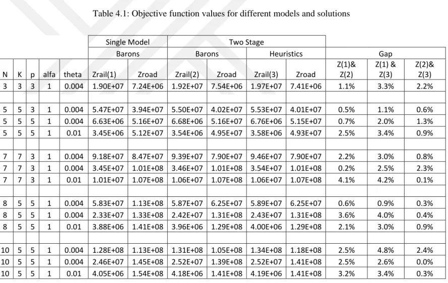
A non-linear model is divided into a two stage model and the model is solved by the heuristics which gives optimal values for the variables. The network is clearly planned and the entrant has the required information. Table 4.1 provides the objective function results for three different solution methods for small problem sizes so that comparison of their performance can be done. Profit of entrant and incumbent is provided in three frameworks with different parameters and network size. Single model is solved using BARONS non-linear solver. Two stage model is solved with two methods. Firstly, two stage model is solved again in BARONS, where after solving the strategic level of the problem, since price and market share are unknown the operational level of the problem is non-linear. Secondly, the iterative heuristics procedure is applied to the problem in Eclipse Java IDE. Objective functions values are compared for these three solution methods and it can be seen that the solution gap among them is negligible with maximum of 5% gap. Heuristics solution shows better results for the objective of entrant profit which shows that its performance is better than other two solution methods.
Table 4.1: Objective function values for different models and solutions
Single Model Two Stage
Barons Barons Heuristics Gap
N K p alfa theta Zrail(1) Zroad Zrail(2) Zroad Zrail(3) Zroad
Z(1)& Z(2) Z(1) & Z(3) Z(2)& Z(3)
3 3 3 1 0.004 1.90E+07 7.24E+06 1.92E+07 7.54E+06 1.97E+07 7.41E+06 1.1% 3.3% 2.2%
5 5 3 1 0.004 5.47E+07 3.94E+07 5.50E+07 4.02E+07 5.53E+07 4.01E+07 0.5% 1.1% 0.6%
5 5 5 1 0.004 6.63E+06 5.16E+07 6.68E+06 5.16E+07 6.76E+06 5.15E+07 0.7% 2.0% 1.3%
5 5 5 1 0.01 3.45E+06 5.12E+07 3.54E+06 4.95E+07 3.58E+06 4.93E+07 2.5% 3.4% 0.9%
7 7 3 1 0.004 9.18E+07 8.47E+07 9.39E+07 7.90E+07 9.46E+07 7.90E+07 2.2% 3.0% 0.8%
7 7 3 1 0.004 3.45E+07 1.01E+08 3.46E+07 1.01E+08 3.54E+07 1.01E+08 0.2% 2.5% 2.3%
7 7 3 1 0.01 1.01E+07 1.07E+08 1.06E+07 1.07E+08 1.06E+07 1.07E+08 4.1% 4.2% 0.1%
8 5 5 1 0.004 5.83E+07 1.13E+08 5.87E+07 6.25E+07 5.89E+07 6.25E+07 0.6% 0.9% 0.3%
8 5 5 1 0.004 2.33E+07 1.33E+08 2.42E+07 1.31E+08 2.43E+07 1.31E+08 3.6% 4.0% 0.4%
8 5 5 1 0.01 3.88E+06 1.41E+08 3.96E+06 1.29E+08 4.00E+06 1.29E+08 2.1% 3.0% 0.9%
10 5 5 1 0.004 1.28E+08 1.13E+08 1.31E+08 1.05E+08 1.34E+08 1.18E+08 2.5% 4.8% 2.4%
10 5 5 1 0.004 2.46E+07 1.45E+08 2.52E+07 1.39E+08 2.52E+07 1.41E+08 2.5% 2.6% 0.0%
4.2.1 CAB data results
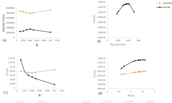
First, the results are obtained by evaluating CAB data set with 25 nodes. Table 4.2 shows the different values of the problem’s variables under different price sensitivity values when the scale effect for the entrant is assumed to be very low α = 0.07 with total number of 290 arcs in the network. Price sensitivity of the customer, or logit pa-rameter (θ ), plays an essential role in the model. Increasing the θ would result in less profit for the entrant, since the customer is less likely to spread its choice over routes in favor of the entrant, and hence, the profit of the intermodal company decreases by more sensitivity of the customer to the price. Also, very low sensitivity, even makes the network more profitable for the entrant than incumbent, since the customer is indiffe-rent to the price, and as a result, entrant can increase its price and obtain more profit. On the other hand, it is interesting to notice that for the incumbent, increasing the θ by starting from very low levels of it (0.001), first is resulting in less profit for the incum-bent but after reaching its minimum profit, more sensitivity bring more profit for the incumbent. This happens because of the optimal θ is capturing the maximum possible market share for the entrant and afterward the shares are falling and the incumbent is taking the benefit. This effect is compensated for the entrant, as the combination of price and market share has a more dominant role in the objective function of the entrant and would result in continuous decrease of the profit for the intermodal firm.
Total market share that entrant can capture in the model, also shows a wide bell curve with respect to the θ . The peak, that is 38% of the total flow in the market, reaches at θ = 0.0035, which is nearly consistent with the findings of Tavasszy et al. that report an optimal logit parameter of 0.0045 for their data [35]. Note that the optimal θ happens at the point that optimal price for the specified route is lowest price. In another word, the optimal θ , is a point in which the captured market share is maximized while the optimal route price is minimized. At extreme points, very small or very large θ is setting the optimal price very high and the market share very low for the entrant. The entrant can achieve 23% profit in the network by only sustaining 2 % of the total cost of the network even if the customers are so sensitive to the price. By accepting barely less than 25% of the network cost, entrant can obtain more than 50% of the profit.
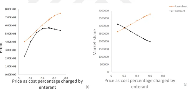
Figure 4.1 demonstrates the profit of both companies and their market shares with respect to the price that entrant charges in term of γ, when θ = 0.0035 and α = 0.07. As discussed before, the transportation energy consumption for rail is estimated to be 0.07 times less than truck transportation. Although for low θ levels the market share
Table 4.2: 25-node CAB data network solutions with α = 0.07. θ Entrant’s Profit Profit % Total Share % Total Cost % 7-3-2-16 Share 7-3-2-16 Price 0.001 1.12E+09 59 28 16 0.30 2778.80 0.002 7.69E+08 53 34 22 0.49 1968.31 0.0025 7.03E+08 51 36 23 0.56 1852.53 0.003 6.43E+08 49 37 24 0.61 1794.64 0.0035 5.69E+08 46 38 24 0.66 1736.75 0.004 4.99E+08 42 37 22 0.65 1736.75 0.005 4.17E+08 36 36 19 0.52 1736.75 0.01 2.59E+08 23 20 2 8.66E-06 2547.23
of the rail is more than the road’s, its profit is always less than incumbent’s profit. Higher prices means less market share for the intermodal and at the same time more profit, since increasing the price would boost the objective function, until a maximum objective level is achieved and after that the profit decreases, since the market share fall is no longer tolerable for the objective function. This balance of price and market share is essential and its level can be determined by the optimal γ which is 0.5 here.
Figure 4.1: Profit and market share levels for rivals with respect to price.
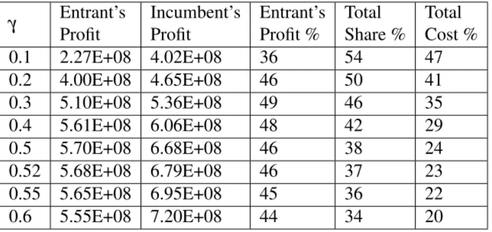
The effect of different prices on the solution can be seen in Table 4.3. In this para-meter setting the optimal price is when γ = 0.5. But lower or higher prices can also be charged with different managerial targets. For instance, one important target can be market share goal for the intermodal shipment. If the network would rather to carry out more than half of the freights through intermodal company, then the optimal pri-cing strategy should be deviated from 50% revenue on cost to only 20%. In another words, government or social planner has to subsidize the difference for the intermodal company which is 42% of its profit.
Table 4.3: 25-node CAB data network solutions with α = 0.07 and θ = 0.0035. γ Entrant’s Profit Incumbent’s Profit Entrant’s Profit % Total Share % Total Cost % 0.1 2.27E+08 4.02E+08 36 54 47 0.2 4.00E+08 4.65E+08 46 50 41 0.3 5.10E+08 5.36E+08 49 46 35 0.4 5.61E+08 6.06E+08 48 42 29 0.5 5.70E+08 6.68E+08 46 38 24 0.52 5.68E+08 6.79E+08 46 37 23 0.55 5.65E+08 6.95E+08 45 36 22 0.6 5.55E+08 7.20E+08 44 34 20
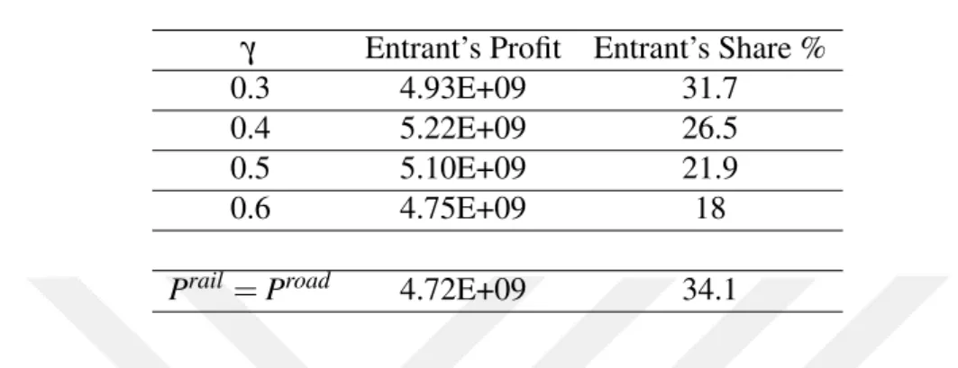
An interesting case is when the price of both firms are equal. market share in each route spreads as half (50%) but total market share that entrant is capturing is nearly 40%. Assuming equal prices, with the mentioned parameter sets, the profit of the entrant is 30% more than incumbent’s profit and the intermodal firm can capture 40% of the mar-ket by accepting to operate on 30% of the total network cost. The model suggests that although the service price that both shipments charge are equal, still total market share are not equal, since truck customers prefer to send their freights with higher speed which is embedded in the model. Constraint (2.10), suggests that the entrant would not operate in the situations that the scale effect cannot make a more convenient route for the entrant. It is assumed that more scale effect would effect the timing inversely as the time can be achieved by only dividing the distance by velocity. Hence, under equal prices, still 60% of the customers would prefer to chose road as their movement option, under the specified parameters.This happens because of the effect of the strate-gic optimization level and the facilities that intermodal firm is active in them. Further, in an extreme case, this assumption is relaxed that will be analyzed in the upcoming sections.
4.2.2 Turkish network solutions
Turkish network, as mentioned before, contains 81 nodes as origin destination demand points and also 43 rail station nodes that are being considered as hub facility points. This data of the real applications in the ground enables us to analyze the problem more realistically. On the contrary to the most of the related studies in the literature, here the distances of existing rail stations are incorporated to the model. Despite its comp-rehensiveness, large size of the problem is the struggle that solution contains a vast number of variables with this data set. Moreover, four index variables are making the solution procedure heavy and exhaustive. To overcome, two stage solution approach
enables the model to be solved in a more flexible manner with accurate results.
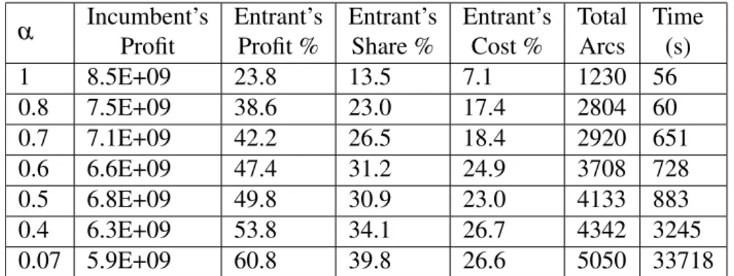
Table 4.4 shows the obtained solution for different levels of scale effect or inter hub discounts (α) for the intermodal transport, when 10 hubs are expected to open and the logit parameter is 0.004. It is obvious that more number of operating hubs, escalates the profit of the entrants. So, as an standard number of hubs, 10 is selected for ease of comparison.
Scale effect is the source of advantage for the intermodal firm to enter the competi-tion. It is clear that lower α would result in better condition for the entrant generally with more profit for the entrant and less for incumbent specifically. When α is one, there is no discount for the intermodal transport, however, there is nearly 24% pro-fit for the entrant with only 7% cost. This happens, since the origin destination cities also can contain hubs inside them. So, when there is no sale effect, still those hubs can operate and transfer freights from their own demand point cities. The entrant can achieve approximately 50% of the network’s profit by only spending less than 25% of the network’s cost by reasonable levels of scale effects.
Lower α opens more opportunity for the entrant, more profit and more market share which is inevitably increasing the cost as well; also, the optimal price decreases with lower α generally. It also makes the network on which the entrant is working wider, as more routes are available because of the less cost of the route that is provided by the entrant. As operating routes increases, the solution time of the model also rises such that it can be seen that for very small numbers of α the solution time is almost ten times more than when the scale effect is 0.4. Also, decreasing the α from 0.8 to 0.7, inflates the solution time to more than 10 times.
It is interesting to notice that, α = 0.5 is the point in which the balance of market share and cost are changing. as α decreases, more routes are involved in the entrant’s network and hence, market share increases with cost. But when discount factor is decreased from 0.6 to 0.5, the effect of inter hub discount makes the toatl aggregate cost of the entrant to fall instead of rise, although the market share is still going up.
On the contrary to the CAB data, in more realistic data set, it can be seen that the profit of the rail is close or more than the road’s with reasonable α levels. for scale effects of less than 0.6, the entrant can achieve more profit than its rival.
Table 4.5 demonstrates the solutions for different logit parameters when the inter hub discount is 0.7 and 10 hubs are expected to be opened. Note that when the scale effect is fixed, the strategic level of the problem does not change and by changing the logit