Γ }¥ Υλ\Υ о “’ 5'чу ¿ í-'í ΠΥΥΛ ■' Й.І-І" Л4Ч), Ч í W>o,A ■ VM«■ >**'. í'l *>M · “*■«)·*■ д а :í ■■*■· , *^·· ; ' ОД" .:^;ϊΐ.ί3!-:ΐϋ· '7 -C^ '> :* {“·?*■ ;*/ ¿ 3 d • г 6 8
QUALITY MEASUREMENT PLAN USING MONTE
CARLO METHODS
A T H E S I S S U B M I T T E D T O T H E D E P A R T M E N T O F I N D U S T R I A L E N G I N E E R I N G A N D T H E I N S T I T U T E O F E N G I N E E R I N G A N D S C I E N C E S O F B I L K E N T U N I V E R S I T Y IN P A R T I A L F U L F I L L M E N T O F T H E R E Q U I R E M E N T S F O R T H E D E G R E E O F M A S T E R O F S C I E N C EBy
Faker Zouaoui
May, 1997
cSlB
J238
1
ЭЭ^I certify that I have read this thesis and that in my opinion it is fully adequate, in scope and in quality, as a thesis for the degree of Master of Science.
Assoc ler(Supervisor)
I certify that I have read this thesis and that in my opinion it is fully adequate, in scope and in quality, as a thesis for the degree of Master of Science.
Prof. Asad Z^an(C o-supervisor)
I certify that I have read this thesis and that in my opinion it is fully adequate, in scope and in quality, as a thesis for the degree of Master of Science.
Approved for the Institute of Engineering and Sciences:
Prof. Dr. Mehmet Baf
Ill
A B S T R A C T
QUALITY MEASUREMENT PLAN USING MONTE
CARLO METHODS
Faker Zouaoui
M.S. in Industrial Engineering Supervisor: Assoc. Prof. Ulkii Gürler
Co-supervisor: Prof. Asad Zaman May, 1997
This study considers the Quality Measurement Plan (QM P), a system im plemented for reporting the quality assurance audit results to Bell system management. QMP is derived from a new Bayesian approach to the empir ical Bayes problem for Poisson observations. It uses both the current and past data to compute estimates for the quality of the current production. The QMP estimator developed by Hoadley in 1981 is based on many com plicated approximations. Sampling approaches such as the Gibbs sampler and Importance-sampling are alternative techniques that avoid these approxima tions and permit the computation of the quality estimates through Monte Carlo methods. Here we discuss the approaches and the algorithms for im plementing some Monte Carlo-based approaches on the QMP model. We also show via simulation that although the QMP algorithm can be computationally more convenient, the sampling approaches mentioned above give more accurate estimates of current quality.
K ey words: QMP, Hierarchical Bayes, Gibbs Sampler, Importance-Sampling,
IV
ÖZET
MONTE-CARLO YÖNTEMLERİNİ KULLANARAK
k a l i t e
Ö
l ç ü m p l a n iFaker Zouaoui
Endüstri Mühendisliği, Yüksek Lisans Danışman: Doçent Ülkü Gürler Ortak Danışman: Profesör Asad Zaman
Mayis, 1997
Bu çalışma, kalite güvencesi denetim sonuçlarının Bell sistem yönetimine ak tarılması amacıyla yürütülen ’’ Quality Measurement Plan (QM P)” (kaliteölçüm plani’ ni) ele almaktadır. QMP, Poisson gözlemler için ampirik Bayes problem ine yeni bir Bayes’ci yaklaşımdan türetilnıiştir. Bu yöntem, ürün kalitesini tah min etmek için hem şimdiki hem de geçmiş verileri kullanmaktadır. Hoadley’in 1981’de geliştirdiği QMP tahmin edicisi bir dizi karmaşık ve yaklaşık hesapla malara dayanmaktadır. Gibbs örnekleyicisi ve önem örneklemesi gibi örnekleme yöntemleri bu yaklaşıklık gereğini ortadan kaldermakta ve kalite tahmin edi cilerinin hesaplanmasında Monte-Carlo tekniklerinin kullanılmasına izin ver mektedir. Bu çalışmada QMP modelinde Monte-Carlo tekniklerine dayalı bazı yaklaşımların denenmesi için algoritmalar ve yaklaşımlar tartışılmaktadır. Simülasyon sonuçlarımız göstermiştir ki, QM P algoritması hesaplama acısından daha etkin kullanılmış olmakla birlikte, örnekleme yaklaşımları mevcut kalitenin daha doğru bir tahminini vermektedir.
Anahtar Sözcükler: QMP, Hiyerarşik Bayes, Gibbs Örnekleyicisi, Önem
VI
A K N O W L E D G E M E N T S
I would like to express my gratitude to Prof. Asad Zaman due to his supervi sion, suggestions, and understanding to bring this thesis to an end.
I am especially indebted to Assoc. Prof. Ülkü Gürler for her invaluable guidance, and encouragement.
I would like to thank Prof. Halim Doğrusöz for showing keen interest to the subject matter and accepting to read and review this thesis.
I cannot fully express my gratitude and thanks to Çiğdem Gültekin and my parents for their morale support and encouragement.
I would also like to thank Souheyl Touhami, Alev Kaya, Maher Lahmar, Tijani Chahed, and Mehdi Bejar for their friendship and support.
Contents
1 Introduction 1
2 The Quality Measurement Plan (Q M P ) 5
2.1
Introdu ction...5
2.2
Statistical Foundations of Q M P ...6
2
.2.1
The QMP Model ...8
2
.2.2
Posterior Distribution of Current Q uality...10
2.3 Mathematical Derivation of Q M P ... 13
2.3.1 Exact Solution 13
2
.3.2
The QMP Formulae 14 2.4 Pros and Cons o f the QMP 19 3 M onte Carlo-Based Approaches to Calculating Marginal den sities 21 3.1 Introdu ction... 213.2 Monte Carlo A pp roa ch es... 23
CONTENTS viii
3
.2.1
Substitution or Data-Augmentation A lgorith m ... 233
.2.2
Substitution S a m p lin g ... 253.2.3 Gibbs S a m plin g... 27
3.2.4 Relationship between Gibbs sampling and substitution sa m plin g... 29
3.2.5 The Rubin Importance Sampling A lg o r it h m ... 31
3.3 Density E s tim a tio n ... 33
3.4 Sampling I s s u e s ...
35
3.4.1 The Griddy-Gibbs Sampler 36 3.5 Convergence I s s u e s ...
37
3.5.1 “Gelfand, Hills, Racine-Poon and Smith” methods . . . . 38
3.5.2 Tanner and Wong methods... 39
3.5.3 The Gibbs S t o p p e r ... 40
3.6 Gibbs Sampling with Improper Posteriors 41 3.7 Summary D is c u s s io n ...
43
4 Q M P using M onte Carlo Methods
44
4.1 The Hierarchical Bayes M o d e l... 444.1.1 Model 1 ... 44
4.1.2 Model 2 ... 46
CO N TEN TS ix
4.2.1 Gibbs Sampler Algorithm 48
4.2.2 Importance-Sampling A lgorithm ... ... 49 4.2.3 Implementation I s s u e s ... ... 50 4.3 Simulation S t u d y ... ... 53 4.3.1 Simulation Design... ... 53 4.3.2 Simulation R e s u lt s ... ... 54 5 Conclusion 56
List of Figures
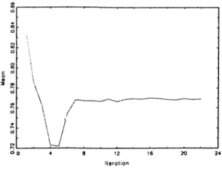
4.1 The mean of 9q across iterations. 51
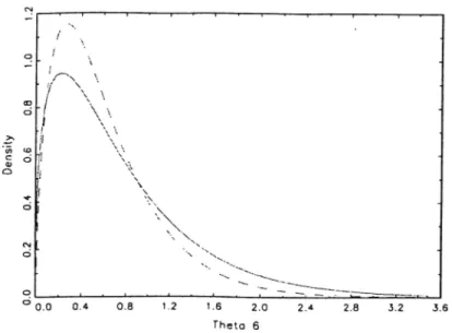
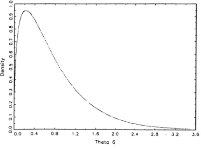
4.2 The posterior density of de. The dashed line represent iteration 5, and the solid line represent iteration 10. 52 4.3 The posterior density of 9^· The dashed line represent iteration
List of Tables
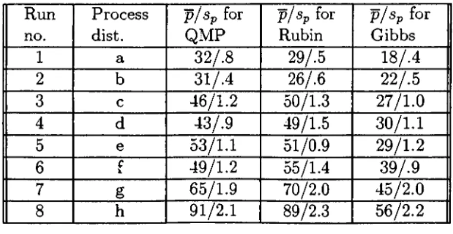
4.1 Equivalent Defects in Keys of Telephone sets - Shreveport 50 4.2 Simulation R e s u l t s ...
55
Chapter 1
Introduction
Thousands of products are designed by Bell laboratories and produced by A. T.
&c T. (formerly called Western Electric). For quality control purposes, a u d if
samples are taken from each product and tested for defects. The main objective o f the quality assurance department is to estimate the quality of the product from the sample, and to decide whether the product meets standard quality requirements or not.
The statistical foundations o f the audit ingredients were developed by She- whart. Dodge, and others, starting in the 1920’s and continuing through to the middle 1950’s. This work was documented in the literature in[41, 40, 10,
11
] and evolved into the T-rate system. The basic idea behind the T-rate system is that observed quality results can be statistically compared to the standards, using a statistic called the T-rate.For a given production period, let Q denote the total number of defects that are observed in all the inspections conducted on all the products. Because there are quality standards for each set o f inspections on each product, it is possible to compute the standard mean and variance of Q imder a given standard, denoted hy E {Q \
5
'),and (Q | S '). The T-rate isC H A PTER 1. INTRODUCTION
T-rate = g ( Q | S ) - 9
It measures the difference between the observed result and its standard in units o f statistical standard deviation. The T-rate is plotted in the control chart. The control limits of ± 2 are reasonable under the assumption that Q
has an approximate normal distribution. Then the standard distribution of Q
is the “standard normal” , and excursions outside the control limits are rare under standard quality. For large audit samples, this approximation follows from the central limit theorem. As we shall see, the approximation is poor for small samples.
The advantage of the T-rate is its simplicity. It can be calculated manually. Exceptions can be identified by inspection. The fact that the T-rate has been used for so long is a testimonial to its advantages. However, the T-rate does have problems. The T-rate is not a direct measui'e of quality. A T-rate of
-6
does not mean that quality is twice as bad as when the T-rate is -3. The T-rate is only a measure o f statistical evidence with respect to the hypothesis o f standard quality. To be specific, suppose the quality standard requiresOf. = 1. If an estimate 6t =
0.99
has standard deviation 0.003, it is three standard deviations away from the null, and we will reject the null. However, the dereliction does not appear quantitatively serious. This is quite different from a situation where 6t = 0.05 and has standard deviation 0.05, and both are different from a case where Of, = 0.5 and the standard deviation is 0.25. In the first case we know for sm'e that the quality is slightly below normal. In the second we know for sure that the quality is way below normal, and in the third, we have a lot of uncertainty as to the real quality. In aU three cases we reject the null hypothesis, and no further information is provided. Many other problems relating the T-rate system are described in detail in [22].In the late seventies, research has been carried out to evaluate the appli cation of modern statistical theories to quality assurance. An important idea is summarized in an article by Efron and Morris[13] which explains a paradox
discovered by Stein[43]. When you have samples from similar populations, the individual sample characteristics are not the best estimates o f the individual population characteristics. Total error is reduced by shrinking the individ ual sample characteristics part way towards the grand mean over all samples. Efron and Morris used baseball batting averages to illustrate this point. But the problem o f estimating percent defective in quality assurance is the same problem. And you are always concerned with similar populations-for example, the population of design-line telephones produced for each o f several months. This idea was originally explored in Hoadley[
21
]. The idea has now evolved into the Quality Measurement Plan(QM P).QM P was implemented throughout Western Electric in 1981 and by Bell core in 1984. It is an Hierarchical Bayes(HB) approach to the control chart. It replaced the T-rate system described briefly above. Many of the advan tages of the QM P relate to the disadvantages of the T-rate system. The main advantage is that unlike the T-rate, QM P uses past and current data to pro vide an inference about current quality not past quality. Hoadley[
22
] gives the rationale for changing the T-rate system.Chapter
2
gives the statistical foundations of the QMP. The QM P model is described along with the QM P algorithm for estimating the posterior dis tribution of current quality. The methods developed by Hoadley in solving the QMP model might be the only methods available at that time in solving HB problems. Although they are computationally efficient, they are based on many complicated approximations and they may not work on all data sets. However, with the developments in computing power, many other techniques have emerged in the late 80’s and 90’s in order to calculate posterior distribu tions in HB problems. They are based on sampling approaches using Monte Carlo methods.CHAPTER 1. INTRODUCTION 3
Chapter 3 gives a unified exposition o f these techniques and evaluates their potential for HB problems. Most of the implementation issues such as the sampling and convergence issues are discussed thoroughly in this chapter.
in chapter 3 on the QMP model. Some small modifications are added to the model in order to reformulate it in HB terms. Moreover, we show via simulation that the new implemented algorithms performed better than the existing QMP algorithm.
C H A P TER 1. INTRODUCTION 4
Finally in chapter 5, we summarize the different aspects of our study. We also underline future extensions of this work.
Chapter 2
The Quality Measurement Plan
(QM P)
2.1
Introduction
This chapter is not intended to document QMP. We are only interested in the mathematics o f the QMP and how it relates to the Hierarchical Bayes. Readers who are interested in the rationale for changing the rating system, the operating characteristics of QMP and its reporting format may refer to Hoadley[
22
, 23], and Bellcore[lj. Section2.2
illustrates the statistical founda tions of the QMP. Here we describe the QMP model and give the form of the posterior distribution o f current quality. Section 2.3 shows that it is computa tionally impractical to derive the exact posterior distribution of current quality and gives a heuristic algorithm for QMP. Finally, Section 2.4 provides the pros and cons in developing the heuristic algorithm of the QMP.2.2
Statistical Foundations of QMP
For the purpose of reporting quality of an audit results to management, the products are grouped into rating classes. The results of all the inspections associated with this rating class are aggregated over a time period called a
rating period. In Bell laboratories a rating period is about six weeks and there are about eight rating periods per year. The defects assessed in each rating period are transformed into demerits or defectives or may remain as simple unweighted defects. In an audit based on demerits, each defect assessed is assigned a number of demerits:
100
, 50,10
, or1
for A, B, C, or D weight defects, respectively. In an audit based on defectives, all defects foimd in a unit o f product are analyzed to determine if the unit is considered defective.A complicating factor in the analyses of audit results is that defects, defec tives, and demerits are different. But in fact they are not different; because, for statistical purposes, they can all be transformed into equivalent defects that have approximate Poisson distributions. Suppose we have a quality mea sure
Q
(Total defects, defectives, or demerits). Let Eg and Vg denote the standard mean (called expectancy) and variance o fQ.
So the T-rate is is T = { E g - Q ) /y /V g .Now define
CHAPTER 2. THE QUALITY MEASUREMENT PLAN (QMP) D
X
= equivalent defects =Q
Vs/Eg' and e = equivalent expectancy = standard mean ofX.
EgVg/Eg
Vg'If all defects have Poisson distributions and are occurring at 6 times the standard rate, then it can be shown that
E[x\e\ = v[x\e] = ee.
Hence, X has an approximate Poisson distribution with mean e9.
As an example, consider the demerits case. The total munber o f demerits has the general form
D = J2 w iX i,
where the Wi's are known weights and the X iS have Poisson distributions. Assume that the mean of X^ is CiO, where Cj is the standard mean o f X{ and 9
is the population quality expressed on an index scale. So 9 = 2 means that all types of defects are occuring at twice the rate expected.
The mean and varinace o f D are
CHAPTER 2. THE QUALITY MEASUREMENT PLAN (QMP) (
E { D ) = Y ,W iE {X i) Y^W i{ei9) 9Es, and V {D ) = Y ^ w ^ V iX ,) = evs,
where Eg and are the standard mean and variance, respectively, of D.
These are the numbers that would be published in the official list o f standards called the Master Reference list.
CHAPTER 2. THE QUALITY MEASUREMENT PLAN (QMP)
The mean and variance of equivalent defects, X , are
E { X ) = E { D ) Vs/Es dEs V s/E , — Oe. and U ( A ) = V j P ) [V s /E ,f eV sE ,
\/2
^ 3 = 9e.The mean and variance of X are equal; so, X has an approximate Poisson distribution with mean eO. Of course, it is not exact, because X is not always integer valued. A similar analysis works for the defectives case. So, any ag gregate o f demerits, defectives, or defects can be transformed into equivalent defects. Just use the standard expectancy and variance as illustrated above for demerits.
2.2.1
The Q M P Model
For rating period i, let Xt = equivalent defects in the audit sample, Cj = equivalent expectancy of the audit sample, and 9t = population index as defined previously. Based on our previous discussion , we assume that
Xt\9t'^ Poisson {et9 t).
decided to restrict his use o f past data to five periods. The main administrative reason is that the T-rate system used the past five periods.
A consequence of using only six periods of data is that no useful inference can be made about the possible complex structure in the stochastic process of ^t’s. So we assume simply that the Ot's are a random sample from an unknown distribution called the process distribution. Furthermore, six observations are not enough to make fine inferences about the family of this unknown distribu tion. So for mathematical simplicity we assume it to be a gamma distribution with unknown mean Ѳ (called the process average) and variance
7
^(called the process variance). The gamma distribution is used because it is the natural conjugate prior to the Poisson distribution and it is a reasonable parametric model of a unimodal distribution on the nonnegative real numbers. The choice of a imimodal distribution reflects the experience that usually many indepen dent factors affect quality; so there is a central limit theorem effect.The model so far is an empirical Bayes model. The parameter of interest is the current population index, Ѳт, which has a distribution called the process distribution. Bayesians would call it the prior distribution if it were known. But we must use all the data to make an inference about the unknown process distribution. So, the model is called empirical Bayes.
Efron and Morris[
12
] take a classical approach to the Empirical Bayes model. They use classical methods of inference for the unknown process distri bution. QM P is based on a Bayesian approach to the empirical Bayes model. Hence, the model is called Hierarchical Bayes (HB). Each product has its own process mean and variance. These vary from product to product. By analyzing many products, we can model this variation by a prior distribution for {Ѳ, .Summarizing, the QMP model is
CHAPTER 2. ТЫЕ QUALITY MEASUREMENT PLAN (QMP) У
Xt I Poisson {et9t) , i = 1 , . . . , T,
/02
^2
\9t ~ Gamma - r , т г Ьr y Л
CHAPTER 2. THE QUALITY MEASUREMENT PLAN (QMP) 10
~ prior distribution p (O. .
This is a full Bayesian model. It specifies the joint distribution of all vari ables. The quality rating in QMP is based on the posterior distribution of 9t
given X = ( x i , . . . , r t r ).
2.2.2
Posterior Distribution of Current Quality
We show in the next section that it is computationally impractical to derive the exact posterior distribution of 9t. The best we can do is approximate the posterior mean and variance of 9t.
The posterior mean and variance are derived in Section IV of Hoadley[
22
]. A brief discussion o f how to derive them is given in the next section. The posterior mean is9
t= E {9
tI x)
= ujx9 T (1 — ¡t· where h 9 UJj' U)j' = Xt /^T-= E { 9 \ ^ ) ,= E {
ujtI x),
_
9 je T - \ - ' fThe posterior mean, 9^^ is a weighted average between the estimated process average, 9, and the defect index, /7·, of the current sample. It is the dynamics of the weight, that makes the Bayes estimate work well. For any i, the sampling variance o f / r is
CHAPTER 2. THE QUALITY MEASUREMENT PLAN (QMP) 11
et
=
3
{etOt)= Ot/et.
The expected value of this is
E [ e t / e t ] = e / e t .
So the weight, u t, is
[expected sampling variance]
[expected sampling variance] + [process variance] ’
If the process is relatively stable, then the process variance is relatively small and the weight is mostly on the process average; but if the process is relatively unstable, then the process variance is relatively large and the weight is mostly on the current sample index. The reverse is true o f the sampling variance. In other words, ujx, is a monotonie function of the ratio of expected sampling variance to process variance. The posterior variance of 9j· is
Vy “ (1 — ^t) 9t/ ej" 4" {9 ] x) 4” ^ (^t I ·
If the process average and variance were known, then the posterior variance o f 9t would be
(1
— Ut) 91·/ej·. So the first term is just an estimate o f this. But since the process average and variance are not known, the posterior variance has two additional terms. One contains the posterior variance of the process average and the other contains the posterior variance of the weight.If the process average and variance were known, then the posterior distribu tion would be gamma (see the next section). So we approximate the posterior
CHAPTER 2. THE QUALITY MEASUREMENT PLAN (QMP) 12
distribution with a gamma fitted by the method of moments. The parameters of the fitted gamma are
e l
V = Shape parameter = -rf-,
Vj·
T = Scale parameter Vt
1 ^'
and the posterior cumulative distribution is
P r(
6
>r < y I x) = Gy{y/T)The QM P formulae for the above terms are given in Section
2
.3
.2
. These are derived by Hoadley[22, 23]. The actual scheme used by Hoadley begins with the formulae above, but with substantial developments of several types. He used some moments o f the marginal distribution of which is a negative binomial distribution (See the next section) to calculate weighted average es timates of the hyperparameters. Moreover, he calculated some empirical prior distributions for the hyperparameters. He did not use the exact forms of these distributions, but just some o f their characteristics such as mean, variance, and mode. A thorough discussion on these developments is given in Hoadley[22
].The main objective of Hoadley in developing the QM P formulae at that time is to sell them to the management and to the engineers. Many of the developments in his estimation procedures were in fact ad-hoc, these are listed in Section 2.4. These were quite complex, but were a product o f the necessity to be sufficiently better than the earlier quality management plan in effect as to be bureaucratically acceptable, and to be easy to compute.
CHAPTER 2. THE QUALITY MEASUREMENT PLAN (QMP) 13
2.3
Mathematical Derivation of QMP
2.3.1 Exact Solution
We are interested in the posterior distribution o f 9t given x, for the model de scribed above. For mathematical convenience let us define the h\"perparameters
n2 2
a and /9 as: a = ^ and /3 =
Given Xt \ Ot ^ Poisson(e(^t) and 6t ~ Gamma(o:,,5), then the posterior density o f 6t is also gamma, and the marginal density of Xt is negative binomial. The following calculation factorizes the joint density of Xt and 6t into the product o f the marginal of Xi and the posterior of 9t given
Xt-f(x, , e, ) = f { x , \ e , ) y . f ( e , )
= {PW e,)xG(a,/J)}
“ x,\ ) ' ' [ p o r { a ) ) U ! r ( Q ) ( l / / 3 + e , f + V l(l//J + e,)-<*'+“' r ( x , + a). = / i^t) X f{0t\ Xt) = { W B ( Q , ; 3 ) x G ( i , + a , ( e , + l//J) -') } Now./
OO / Pr(^T < y \ o t , p , xr)p{oi, p \'x ) da dp,TO O 0 «/ 0where p { a ,P \ x ) is the posterior distribution of a ,P given x.
We know from the above calculation that the distribution of 9t given a ,P
and Xt is gamma; so Pr(^
7
’ < y |a ,p ,X r ) can be expressed in terms o f an incomplete gamma function.CHAPTER 2. THE QUALITY MEASUREMENT PLAN (QMP) 14
p(a, ^ I x) = I x) L ( x I a ,^ )
/o” / o ° p ( « . / ? I x)-C'(x I d a d (5 '
where p {oi,P \ x ) is the prior density o f { a ,p ) and L (x |a ,P ) is the like lihood function. We know from above that Xt given a ,P is negative binomial. Hence,
L ( x l a , / J ) = n ‘=“ ' ( W ) “ r ( x , + a)
t J i x ,\ T { a ) { l / 0 + e , r ‘* °
So the posterior distribution of 9t is a complex triple integral that has to be inverted to compute the QM P box chart. The posterior mean and variance of
9t can be expressed in terms of several double integrals. There are more than
1,000
rating classes that have to be analyzed each period, so computational efficiency is important. This is why heuristic algorithms were developed for the QMP model.2.3.2
The Q M P Formulae
Two heuristic algorithms have been implemented for QMP. The first was de rived by Hoadley[22] and the second, which is currently used at Bellcore, was derived by Hoadley[23]. For completeness, we state the formulae from Hoadley[23] that are needed to implement the QMP estimator. The formulae look complex, but they are algebraic and easily programmable.
As explained before, the QMP model has a prior distribution on {9, 'p). The parameters of this prior that we use are 9q = prior mean of 9, Uq = prior variance o f 9,
7
o = prior mean o f7
^, and7
^^.^ is defined by P r {7
^ < 7max} = -95. We require a technical constraint Uq >7
q, which is caused by some o f the priorinformation being implemented in the algorithm as artificial data:
CHAPTER 2. THE QUALITY MEASUREMENT PLAN (QMP) 15
= Oq/ (uo - 7o)
and
Xq = prior defects
= ^0^0.
The default priors used in the current Bellcore implementation of QMP are
do = 1, Uq = 3.05,
7
o = .55, and7
max = 2.2. These were arrived at by analysis o f factory quality-audit data for many products.The audit data for i = 1, 2 , . . . , T is the following:
Qf = Attribute quality measure in the sample period t
(total defects, defectives, or demerits),
Egt = Expected value of Qt given standard quality,
Vst = Sampling variance of Qt given standard quality.
For each period compute the following: Equivalent defects: Xt =
Qt
V j E s t Equivalent expectancy: et = V,3tCHAPTER 2. THE QUALITY MEASUREMENT PLAN (QMP) 16
Sample index:
h = Xt/eu
Weighting factors for computing process average and variance:
bt 4>o ft 9t 7o +
2
+670/^0
ilbt,1
/ {(pobj - [^oet]) Corresponding weights: Vt — f t ! Z ! /(> i=0 T 9t = gt/ E 9t-t=oOver all periods compute the following: Process average:
& = Yff=oPth,
Average sampling variance:
= E L , ft ( « / f t ) ,
Total observed variance:
CHAPTER 2. THE QUALITY MEASUREMENT PLAN (QMP) 17
Shape parameter for the sampling distribution of V :
tti —
Z L i O t i O o / ^
Shape parameter for the prior distribution of a; = cr^/ (a +
7
)do —
In (
20
)In [1 + ’
Shape parameter o f the posterior distribution o f u>:
(1
= oq "I” n1
.Adjusted total variance:
= (ai/a) U.
Adjusted variance ratio:
R =
Bayes adjustment factor used to keep the estimator process variance posi
tive:
B = E T = i T { i ) ,T { 0 ) = l, T { i) =
a -f z.
T (m) is the term in which either
- 7
T (m) > 10^ or T (m) <
10
,F = 1 + {1/B),
CHAPTER 2. THE QUALITY MEASUREMENT PLAN (QMP) 18
Posterior variance of u;:
G = i
rii±ll_F+l— L-l
if R > o ,
(a+
2
)(a+l)'^ if ^Current sampling variance:
Sampling variance ratio:
= e/e r, Tt = Process variance: 7 = F S ‘^ - a ^ if i ? >
0
, (j^/o if il =0
,Average shrinkage weight:
Q = cr^/ {a^ + 7^^
Shrinkage weight for the current period:
wt = (Jt! {(^t + 7^) ,
Best measure of current quality:
E (Ox
I x) =u!x6
-|- ( l —I
t— Ox,
CHAPTER 2. THE QUALITY MEASUREMENT PLAN (QMP) 19 V {9t \'x) =
(1
— Qt) 9t! t=o f + et [ ( r r - l ) c D + i r2.4
Pros and Cons of the QMP
\Iany of the advantages of QMP relate to the disadvantages of the T-rate system. QM P does not use runs criteria, but uses the actual equivalent defects observed. It uses past and current data to make an inference about current quality not past quality. For example, under QMP a rating class is Below Normal if the posterior probability that the product is substandard^ exceeds 0.99. However, under the T-rate system a rating class is Below Normal if the current T-rate is below —3 and at least one of the previous five T-rates is below — 2. The T-rate system uses numerous patchwork rules to exploit information in the past history of the production process such as the rule of Below Normal. But the information is not used in an efficient way. A situation where there is long past experience on the same or similar parameters is ideally suited to the use o f Bayesian methods. Another advantage of the QMP on the T-rate system is that it provides a lower producer’s risk and consequently a more accurate list of exceptions (see Hoadley[22]). Finally, unlike the T-rate statistic, the QMP report format met the needs of the operating companies.
From the previous section it should be clear that the Hierarchical Bayes (HB) estimator is quite difficult to obtain. For this reason, applications of HB estimation have been very few. See the study by Nebebe and Stroud[29]. Approximating the posterior resulting from the HB analysis requires a lot of numerical integration. There are a number o f different ad-hoc methods for carrying out such approximations, each adapted to particular applications.
CHAPTER 2. THE QUALITY MEASUREMENT PLAN (QMP) 20
Hoadley used a technique like this to compute the QMP estimator. In the past this was the only method of obtaining approximations to HB estimators. How ever, the invention of Monte Carlo approaches such as Gibbs and substitution sampling for computing HB estimators has rendered this type o f approximation considerably less useful than before. So it is probably preferable to calculate the HB estimates by the Monte Carlo techniques rather than approximate it in some ad-hoc fashion which is typically quite complex in itself like in our case.
In the next section, we will describe three Monte Carlo-based approaches put forward in the literature for calculating marginal densities (or posterior densities in HB applications) before applying these techniques to the QMP model.
Chapter 3
Monte Carlo-Based Approaches
to Calculating Marginal
densities
3.1
Introduction
Metropolis, Rosenbluth, Rosenbluth, Teller and TeUer[28] introduced a Monte Carlo-type algorithm to investigate the equilibrium properties of large systems of pai'ticles, such as molecules in a Gas. Hastings[20] used the Metropolis algo rithm to sample form certain distributions; for example Poisson, standard nor mal, and random orthogonal matrices. Besag[2] studied the associated Markov field structure. Geman and Geman[17] illustrated the use of a version o f this algorithm that they called the Gibbs sampler in the context of image recon struction. More recently. Tanner and Wong[44] developed a framework in which Gibbs sampler algorithms can be used to calculate posterior distributions; and Carlin, Gelfand, and Smith[4]; Carlin and Poison[5]; Gelfand, Hills, Racine- Poon, and Smith[14]; Gelfand and Smith[15]; Gelfand, Smith, and Lee[16]; Li[27]; Verdinelli and Wasserman[45]; and Zeger and Karim[49] used the Gibbs sampler to perform Bayesian Computations in various important statistical
CHAPTER 3. MONTE CARLO-BASED APPROACHES TO CALCULATING MARGINAL DENSITIES 22
problems.
In Section 3.2, we discuss three alternative approaches put forward in the literature for calculating marginal densities via Monte Carlo (or sampling) algo rithms. These are (variants of) the data-augmentation algorithm described by Tanner and Wong[44], the Gibbs sampler algorithm introduced by Geman and Geman[17], and the form o f importance-sampling algorithm by Rubin[38, 37]. We note that the Gibbs sampler has been widely taken up in the image- processing literature and in other large-scale models such as neural networks and expert systems, but in general potential for more conventional statistical problems seem to have been overlooked. As we show, there is a close relation ship between the Gibbs sampler and the substitution or data augmentation algorithm. We generalize the latter and show that it is as efficient as the Gibbs sampler, and potentially more efficient, given the availability of distinct conditional distributions. We note that a consequence of the relationship be tween the two algorithms, the convergence results established by Geman and Geman[17] are applicable to the generalized substitution algorithm. Both the substitution and the Gibbs sampler algorithms are iterative Monte Carlo pro cedures. However, we see that an importance sampling algorithm based on that of Rubin[38, 37] provides noniterative Monte Carlo integration approach to calculating marginal densities.
In Section 3.3, we consider the problem of calculating a final form of marginal density from the final sample produced by either the substitution or Gibbs sampling algorithms. In Section 3.4, we propose several methods for sampling from nonconjugate conditional distributions. Moreover, some refer ences are given for the efficient generation of variates from some known dis tributions. In Section 3.5, we propose some techniques useful for assessing convergence of the substitution or Gibbs sampling algorithms. In Section 3.6, we illustrate the effect o f improper priors on Gibbs sampling. Finally, in Sec tion 7 we provide a summary discussion.
CHAPTER 3. MONTE CARLO-BASED APPROACHES TO CALCULATING MARGINAL DENSITIES 23
3.2
Monte Carlo Approaches
In the sequel, we assume that we are dealing with real, possibly vector-valued random variables having a joint distribution whose density function is strictly positive over the (product) sample space. This ensures that knowledge of all full conditional distributions imiquely defines the joint density (e.g., see Besag[2]). Throughout,We assume the existence of densities with respect to either Lebesgue or counting measure, as appropriate, for all marginal and con ditional distributions. The terms distribution and density are therefore used interchangeably. Densities are denoted by brackets, so joint, conditional, and marginal forms, for example appear as [X, T ],
[X
\ K], and [W]. Multiplication is denoted by for example,[X, Y\
= [W | F] * [F ]. The process of integration is denoted by forms such as [X | F] =j [X
\ F, Z, W ]* [Z \ W, F] * [W | F], with the convention that all variables appearing in the integrand but not in the resulting density have been integrated out.3.2.1 Substitution or Data-Augmentation Algorithm
The substitution algorithm for finding fixed-point solutions to certain classes o f integral equations is a standard mathematical tool that has received con siderable attention in the literature (e.g., see Rall[3l]). Its potential utility in statistical problems of the kind we are concerned with was observed by Tanner and Wong[
44
] (who called it the data-augmentation algorithm). Briefly review ing the essence of their development using the notation introduced previously, we have[X]
= / [A I T] . [y]
(3.1)and
CHAPTER 3. MONTE CARLO-BASED APPROACHES TO CALCULATING MARGINAL DENSITIES 24
so substituting (3.2) into (3.1) gives
[X]
=
l [ X \ Y ] * J { Y \ X ' ] [ X ‘]
=
I h(x,x'),[x'\
(3.3)Where h (X , X') = f [X \ Y] * [Y \ X ' ] , with X' appearing as a dummy argument in (3.3), and of course [X] = [ X '] .
Now suppose that on the right side of (3.3), [X'] were replaced by [X]^, to be thought as an estimate of [X] = [X'] arising at the zth stage o f an iterative process. Then, (3.3) implies that for some [X]t-i-i, [X]i-i-i =
J
h{X , X ')*[X ']i = Ih[X]i, in a notation making explicit that Ih is the integral operator associated with h. Exploring standard theory o f such integral operators. Tanner and Wong[44] showed that under mild regularity conditions this iterative process has the following properties (with obviously analogous results for [T]).T W l (uniqueness). The true marginal density, [X], is the unique solution to (3.3).
TW 2 (convergence). For almost any [X]o, the sequence [X ]i, [X ]
2
, . . . de fined by [X]i-i-i = //i[X ]i(i = 0 ,1
, . . . ) converges monotonicaUy in Li to [X].T W (rate),
j
|[X]¿ — [X]| —>■0
geometrically in i.Extending the substitution' algorithm to three random variables X , Y, and
Z, we may write [analogous to (3.1) and (3.2)]
[X) = l i x , z \ Y ] * i Y ] |y| = | i y , x | z | . ( z ) [Z] = J [ Z .Y \ X ] ,[ X \ (3.4) (3.5) (3.6)
CHAPTER 3. MONTE CARLO-BASED APPROACHES TO CALCULATING MARGINAL DENSITIES 25
Substitution o f (3.6) into (3.5) and then (3.5) into (3.4) produces a fixed- point equation analogous to (3.3). A new h function arises with associated integral operator 7^, and hence T W l, T W
2
, and TW 3 continue to hold in this extended setting. Extension to k variables is straightforward.3.2.2
Substitution Sampling
Returning to (3.1) and (3.2), suppose that [X |Y\ and \Y \ X\ are avail able in the sense defined at the beginning of the previous section. For an arbitrary (possibly degenerate) initial density [X]q draw a single X^^^ from
[AT]q. Given since [Y \ X\ is available di'aw ~ | , and hence from (3.2) the marginal distribution of T^^hs =
j
\Y \ X ] * [A”]q. Now,complete a cycle by drawing I . Using (3.1), we then have X (i) ^ = I [ X \ Y ] * [r ]i =
J
h (X ,X ') * [X'lo = h [X]o· Repetition of this cycle produces and X^^\ and eventually, after i iterations, the pair( A « , y ^ W ) such that a: « ^ a ~ [X], and Y ^ [Y], by virtue of TW 2. Repetition of this sequence m times each to the ith iteration generates
m iid pairs ( x f \ Yj^^) { j = 1 , . . . ,m ). We call this generation scheme substi tution sampling. Note that though we have independence across j , we have dependence within a given j.
If we terminate all repetitions at the zth iteration, the proposed density estimate o f [X] (with an analogous expression for [T]) is the Monte Carlo integration
1
^ J = l(3.7)
Note that the Xf'^ are not used in (3.7).
We note that this version o f the substitution-sampling algorithm differs slightly from the imputation-posterior algorithm o f Tanner and Wong[44]. At each iteration l{l =
1
,2
, . . . ,i),they proposed creation o f the mixture densityCHAPTER 3. MONTE CARLO-BASED APPROACHES TO CALCULATING MARGINAL DENSITIES 26
estimate , [X]/, of the form in (3.7), with subsequent sampling from [X]i to begin the next iteration. This mechanism introduces the additional randomness of equally likely selection from the before obtaining an We suspect this sampling with replacement of the was introduced to allow m to vary across iterations, which may reduce computational effort.
The L i convergence of [X]^ to [X] is most easily studied by writing
I\[xl -
[A|| <
I
|[
a]. - [X),| +
The second term on the right side can be made arbitrarily small as i —* oo,
as a consequence of TW 2. The first teiTn on the right can be made arbitrarily small as m —> oo, since [X]j [X]i for almost all X (Glick[19]).
Extension of the substitution-sampling algorithm to more than two ran dom variables is straightforward. We illustrate using the three-variable case, assuming the three conditional distributions in (3.4)-(3.6) are available. Tak ing an arbitrary starting marginal density for X , say [X]o, we draw X^°^ ~
[X]o, ~ [ Z , r |XW], ( r ( i ) , X W ' ) - [ r , X | ZW' j, and finally ~ I A full cycle of the algorithm (i.e., to generate XG ) starting from X^®^) thus requires six generated variates, rather then the two we saw earlier. Repeating such a cycle i times produces (x^®\ Y^'’\
The aforementioned theory ensures that X^‘^ X ~ [X], Y ~ [T], and Z^^ ^ Z [Z]. If we repeat the entire process m times we obtain iid (^Xj^\Yj’’\Zj^^^ {j = l,. .. ,m) (independent between, but not within, j's).
Note that implementation of the substitution-sampling algorithm does not re quire specification of the full joint distribution. Rather, what is needed is the availability o f [X, Z \Y] ,[Y ,X \ Z ] , and [Z, T | X ]. Of course, in many cases sampling from, say, [X, Z \ T] requires, for example, [X|y, Z] and [K | X ], that is, the availability of a full conditional and a reduced conditional distribution. Paralleling (3.7), the density estimator of [X] becomes
CHAPTER 3. MONTE CARLO-BASED APPROACHES TO CALCULATING MARGINAL DENSITIES 27
X
1
m= — f ] \ x \ z f
i m I- ' ^ ^ (3.8)
W ith analogous expressions for estimating [K] and [Z]. convergence of 3.8 to [X] again follows.
For k variables, U i,...,U k, the substitution-sampling algorithm requires
k [k —
1
) random variate generations to complete a cycle. If we run m se quences out to the ith iteration [m ik{k —1
) random generations] we obtain miid k tuples ···, ( i =
1
,··· , m ), with the density estimator for [l/aj{s = l , . . , k ) being
1
^(3.9)
3.2.3
Gibbs Sampling
Suppose that we write (3.4)-(3.6) in the form
[X] = l [ X \ Z , Y ] * { Z \ V ] , [ Y ]
[p] =
llY\x,z].{x\z],{z]
iz]
=
JiziY,x],[Y\x],{x]
(3.10)Implementation of substitution sampling requires the availability of all six conditional distributions on the right side of (3.10), rarely the case in our applications. As noted at the beginning o f Section
3
.2
, the full conditional dis tributions alone, [X |Z ,Y ], [Y \ X , Z ] , and [Z j Y ,X ], uniquely determine the joint distribution (and hence the marginal distributions) in the situations under study. An algorithm for extracting the marginal distributions from these full conditional distributions was formally introduced by Geman and Geman[17] £ind is known as Gibbs sampler. An earlier article by Hastings[20] developedCHAPTER 3. MONTE CARLO-BASED APPROACHES TO CALCULATING MARGINAL DENSITIES 28
essentially the same idea and suggested its potential for numerical problems arising in statistics.
The Gibbs sampler was developed and has mainly being applied in the con text o f complex stochastic models involving very large numbers of variables, such as image reconstruction, neutral networks, and expert systems. In these cases, direct specification of a joint distribution is typically not feasible. In stead, the set o f full conditionals is specified, usually by assuming that an individual full conditional distribution only depends on some “neighborhood” subset of the variables. More precisely, for the set of variables Ui,U<2, ...,Uk,
\U i\U y,i^i\ = [U ,\ U j-,j(iS ,], « =
1
...k. (3.11)where Si is a small neighborhood subset o f {1,2,..., A:}. A crucial ques tion is xmder what circumstances the specification (3.11) uniquely determines the joint distribution. The answer is taken up in great detail by Geman and Geman[17], involving concepts such as graphs, neighborhood systems, cliques, Markov random fields, and Gibbs distributions. Section 3.5 provides also some references to answer this crucial question.
Gibbs sampling is a Markovian updating scheme that proceeds as follows. Given an arbitrary starting set of values U ^\ U ^\ ,U ^\ we draw
r(i)
U2 I . . . , , and so on, up to
Thus each variable is visited in the natural order and a cycle in this scheme requires K random variate generations. After i such iterations we could arrive at {U\\ · ■ ■ -,11^^^. Under mild conditions, Geman and Geman showed that the following results hold.
G G l (convergence). (Ui^^, ■ · ■ [Ui,. . . ,Uk] and hence for each s, C/i') ^ Us ~ [Us] as i ->
00
.In fact, a slightly stronger result is proven. Rather than requiring that each variable be visited in repetitions of the natural order, convergence still follows under any visiting scheme, provided that each variable is visited infinitely often
CHAPTER 3. MONTE CARLO-BASED APPROACHES TO CALCULATING MARGINAL DENSITIES 29
(io).
GG2 (rate). Using the sup norm, rather than L\ norm, the joint density of {Ui \ ■ ■ ■ converges to the true joint density at a geometric rate in i,
imder visiting in the natural order. A minor adjustment to the rate is required for an arbitrary io visiting scheme.
GGS (ergodic theorem). For any measurable function T of C/i,. . . , U* whose
i
expectation exists, lim
7
^ T . - ., E [T ( U i , . . . , C4)).As in the previous section, Gibbs sampling through m replications of the aforementioned i iterations {m ik random variate generations) produces m iid
k tuples (Uij , {j = l , . . . , m ) , with the proposed density estimate for
[Ua] having form o f (3.9).
3.2.4
Relationship between Gibbs sampling and substi
tution sampling
It is apparent that in the case of two random variables Gibbs sampling and sub stitution sampling are identical. For more than two variables, using (3.10) and its obvious generalization to k variables, we see that Gibbs sampling assumes the availability of the set of k full conditional distributions (the minimal set needed to determine the joint density uniquely). The substitution-sampling al gorithm requires the availability o f k {k —
1
) conditional distributions, including all of the full conditionals.Gibbs sampling is known to converge slowly in applications with k very large. Regardless, fair comparison with substitution sampling, in the sense of the total amount o f random variate generation, requires that we allow the Gibbs sampling algorithm i{k —
1
) iterations if the substitution-sampling algorithm is allowed i. even so, there is clearly scope for accelerated convergence for the substitution-sampling algorithm, since it samples from the correct distributionCHAPTER 3. MONTE CARLO-BASED APPROACHES TO CALCULATING MARGINAL DENSITIES 30
each time, whereas Gibbs sampling only samples from the full conditional dis tributions. To amplify, we describe how the substitution-sampling algorithm might be carried out under availability of just the set o f full conditional distri butions. We see that it can be viewed as the Gibbs sampler, but under an io visiting scheme different from the natui'al one. We present the argument in the three-variable case for simplicity. Returning to (3.10), if [X |Y] is unavailable we can create a sub-substitution loop to obtain it by means of
[ Y \ X ] = j [ Y \ X . Z ] * I Z \ X ]
iz\x]
=I [z\x,Y]*iY\x\.
(3.12) (3.13)
Similar subloops are clearly available to create [X |Z] and [Z | T]. In fact, for k variables this idea can be straightforwardly extended to the estimation of an arbitrary reduced conditional distribution, given the full conditionals. We omit the details.
The previous analysis suggests that we could view the reduced conditional densities such as [Y \ X] as available, and that we could thus carry out the substitution algorithm as if all needed conditional distributions were available; however, [Y |X] is not available in our earlier sense. Under the subloop in (
3
.12
), we can always obtain a density estimate for \Y | X ], given any specifiedX , say X^^\ At the next cycle of the iteration, however, we would need a brand-new density estimate for [Y \ X] at X = X^^\ Nonetheless, suppose we persevered in this manner, making our way through one cycle of (3.10). The reader may verify that the only distributions actually sampled from are, of course, the available full conditionals, that at the end of the cycle each full conditional will have been sampled from at least once, and thus that under repeated iterations each variable will be visited io. Therefore, this version of the substitution-sampling algorithm is merely Gibbs sampling with a different but still io visiting order. As a result, G G l, GG2 and GG3 still hold (T W l, TW 2 and TW 3 apply directly only when all required conditional distributions are available). Moreover, there is no gain in implementing the Gibbs sampler
CHAPTER 3. MONTE CARLO-BASED APPROACHES TO CALCULATING MARGINAL DENSITIES 31
in this complicated order; the natural order is simpler and equally good. This discussion may be readily extended to the case of k variables. As a result, we conclude that when only the set o f k full conditionals is available the substitution-sampling algorithm and the Gibbs sampler are equivalent. Furthermore, we can now see when substitution sampling offers the possibility o f acceleration relative to Gibbs sampling. This occurs when some reduced conditional distributions, distinct from the full conditional distributions, are available. Suppose that we write the substitution algorithm with appropriate conditioning to capture these available reduced conditionals. As we traverse a cycle, we would sample from these distributions as we come to them, otherwise sampling from the full conditional distributions.
3.2.5
The Rubin Importaince Sampling Algorithm
Rubin [38] suggested a noniterative Monte Carlo method for generating marginal distributions using importance-sampling ideas. We first present the basic idea in the two-variable case. Suppose that we seek the marginal distribution of X ,
given only the functional form (modulo the normalizing constant) of the joint density [X, Y\ and the availability o f the conditional distribution [A j Fj. Sup pose further (as is typically the case in applications) that the marginal distribu tion o f Y is not known. Choose an importance-sampling distribution for Y that has density [F]^. Then, [AT | F] * [F]^ provides an importance sampling distri bution for [X , Y ) . Suppose that we draw iid pairs {Xi,Y{) {I = 1 , . . . , N) from this distribution, for example, by drawing F/ from [F]^ and Xi from [AT j F] · Rubin’s idea is to calculate r·, = [A^j, F] / ([Aj j F ] * [Fj^) (^ = F . . . , A ) and then estimate the marginal density for [A] by
A 1=1 N
E n
/=1
CHAPTER 3. MONTE CARLO-BASED APPROACHES TO CALCULATING MARGINAL DENSITIES 32
Note the important fact that [X, Y] need only be specified up to a constant, since the latter cancels in (3.14). In other words, we do not need to evaluate the normalizing constant for [A, Y ] . By dividing the numerator and the de nominator o f (3.14) by N and using the law o f large numbers, we immediately have the following.
R1 (convergence). [X] —> [A] with probability
1
as A — oo for almost every A .In addition, if [Y | A ] is available we immediately have an estimate for the marginal distribution of Y : N
E I
^'1
’■·
N Y r , 1=1The successful performance of the density estimator (3.14) depends strongly on the choice o f [T]^ and its closeness to [T]. Thus the suggestion of Tanner and Wong[
44
] in their rejoinder to Rubin, to perhaps use for [T]^ the density estimate created after i iterations of the substitution algorithm, merits further investigation.The extension o f the Rubin importance-sampling idea to the case of k vari ables is clear. For instance, when k = 3, suppose that we seek the marginal distribution o f A , given the functional form of [A, Y, Z] up to a constant and the availability o f the full conditional [A |Y,Z]. In this case, the pair
(Y, Z) plays the role of Y in the two variable case discussed before, and in general we need to specify an importance-sampling distribution [F, Z]^. Nevertheless, if [Y \ Z] is available, for example, we only need to specify
[Z]g. In any case, we draw iid triples {X i,Y i, Z{) {1 = 1 , . . . , N ) and calculate
ri = [A/,yi, Zi] / ([A/ I Fz, Zi] * [Yi, Z i]J. The marginal density estimate for [A] then becomes [analogous to (3.14)]
CHAPTER 3. MONTE CARLO-BASED APPROACHES TO CALCULATING MARGINAL DENSITIES 33 N
E
1-^ I
zj r,
X l=l N E n/=1
(3.15)We note that in the A:-variable case the Rubin importance-sampling al gorithm requires N k random variate generations, whereas Gibbs sampling stopped at iteration i requires m ik generations. For fair comparison o f the two algorithms, we should therefore set N = mi. The relative relationship between the estimators (3.7) and (3.14) may be clarified if resample ,. ■ ., Y^ from the distribution that places mass Vi/ '^ri at V/ (Z = 1 , . . . ,N). we could then replace (3.14) with
1
m[^] = - E
I y/
j=l
(3.16)
So (3.7) and (3.16) are of the same form. Relative performance on average depends on whether the distribution of or Y* is closer to [T]. Empirical work described in Gelfand and Smith[l5] suggested that under fair comparison (3.7) performs better than (3.15) or (3.16). It seems preferable to iterate through a learning process with small samples rather than to draw a one-off large sample at the beginning.
3.3
Density Estimation
In this section, we consider the problem of calculating a final form of marginal density from the final sample produced by either the substitution or Gibbs sampling algorithms. Since for any estimated marginal the corresponding full conditional has been assumed available, efficient inference about the marginal should clearly be based on using this full conditional distribution. The next section presents several methods for dealing with unavailable conditional dis tributions.
CHAPTER 3. MONTE CARLO-BASED APPROACHES TO CALCULATING MARGINAL DENSITIES 34
In the simplest case of two variables, this implies that [X \ Y] and the , m) should be used to make inferences about [X ], rather than imputing Intuitively, this follows, because to estimate [X] using the
requires a density estimate. Silverman[42] provides many techniques to construct a density estimate for [X] based on Xj*^'s. This estimate can be adequate if at the last iteration the number o f replications, m, is large enough. However, such an estimate ignores the knou-n form of [X \ Y] that is mixed to obtain [X]. This alternative density estimate, having the form of (3.9), is better under a wide range of loss functions. The formal argument is essentially based on the Rao-Blackwell theorem. Gelfand and Smith[l5] sketched a proof in the context o f density estimator.
If X is a continuous p-dimensional random variable, consider any kernel density estimator o f [X] based on the Xj*^ (e.g., see Devroye and Gybrfi[
8
]) evaluated at Xq : = ( l / m h ^ ) ^ A 'j(X o ~ xj'^)/^m ], say, where Kis a bounded density on EF and the sequence {hm} is such that as m —>
oo, hjn 0, whereas m h ^ —»· oo. To simplify notation, set Qm ,Xo(^) = ( I / f c ^ ) A [ ( A „ - A ) / h „ ] so that a 5> = (1/m ) De
8
n e7
® = (1
/m ) E ( Q ^ ,x „ ( X f) I By our earlier theory, both a J* and7
J’have the same expectation. By the Rao-Blackwell theorem:
v a r E {Qm,Xo { X \ y ) ) < ( X ) , and hence M S E (
7
,^ ) < M S E ( A ^ ) , where M S E denotes the mean squared error o f the estimate of [Xo]·Now, for fixed Y, as m -y 00, E {Qm,Xo
I
y ) ) № |y ] for almost every Xo, by the Lebesgue density theorem (see Devroye and Gyorfi[8
], p.3). Thus in terms o f random variables we have E {Qm,Xo ( ^I
^ ))[^0
I
^]) so for large m,7
^^ ~ Xo . and M S E (7
^0
) ^ M S E ([X o ].) , and hence Xo is preferred to A^^.The argument is simpler for estimation o i j] = E {T ( X ) ) = j T ( X ) * [ X ] , say. Here, ffi = (
1
/m ) ^ T is immediately seen to be dominated byCHAPTER 3. MONTE CARLO-BASED APPROACHES TO CALCULATING MARGINAL DENSITIES 35
3.4
Sampling Issues
Basic to the implementation o f the Gibbs sampler is the ability to sample from the conditional distribution [Xj |^ j , j
7
^ *] · Carlin and Gelfand[3
] referred to this property as conjugacy. In the terminology of Tanner and Wong[44] it is as sumed that one can sample directly from the augmented posterior distribution.Techniques for the efficient generation of appropriate random variates from conjugate conditionals are described in detail in Devroye[
7
] and Ripley[32]. Gelfand, Hills, Racine-Poon, and Smith[14] presented various examples that are conjugate, but other classes o f problems exist (e.g. nonlinear regression) where the posterior distribution is lacking conjugacy in at least one of the conditionals.Recently, several methods have been proposed for dealing with nonconju gate conditionals via importance sampling or acceptance/rejection approaches. Wei and Tanner[47] presented an importance sampling modification when this simplicity is absent. Carlin and Gelfand[3] and Zeger and Karim[49] presented rejection/acceptance modifications to the Gibbs sampler. Also o f note is the work by Gilks and Wild[18], who used tangent and secant approximations above and below the log-posterior to develop an acceptance/rejection scheme. Acceptance/rejection methods are exact in the sense that they produce sam ples from the required distribution. Possible drawbacks to theses methods include a low acceptance rate, the need to know the normalizing constant for the conditional distribution, and possible restrictions on the distribution (e.g., log-concavity). Nonlinear regression problems for example, may lead to conditionals that are not log-concave and may in fact be multimodal. More over, in nonlinear regression the conditionals typically are known only up to a multiplicative constant. Both importance sampling and acceptance/rejection algorithms require a higher degree o f programming sophistication on the part o f the data analyst and thereby detract from the conceptual simplicity and appeal o f the Gibbs sampler. Specification of an importance sampling function that is easy to sample from, yet provides a “good match” to the density o f in terest, may require the specification of several tuning constants. In the context