11.4
The Root Locus Method
Hitay O¨zbay
Introduction
The root locus technique is a graphical tool used in feedback control system analysis and design. It has been formally introduced to the engineering community by W. R. Evans [3,4], who received the Richard E. Bellman Control Heritage Award from the American Automatic Control Council in 1988 for this major contribution. In order to discuss the root locus method, we must first review the basic definition of bounded input bounded output (BIBO) stability of the standard linear time invariant feedback system shown in Figure 11.22, where the plant, and the controller, are represented by their transfer functions P(s) and C(s), respectively1The plant, P(s), includes the physical process to be controlled, as well as the actuator and the sensor dynamics.
The feedback system is said to be stable if none of the closed-loop transfer functions, from external inputs r and v to internal signals e and u, have any poles in the closed right half plane, Cþ:¼ fs 2 C : ReðsÞ > 0g. A necessary condition for feedback system stability is that the closed right half plane zeros of P(s) (respectively C(s)) are distinct from the poles of C(s) (respectively P(s)). When this condition holds, we say that there is no unstable pole–zero cancellation in taking the product P(s)C(s) ¼ : G(s), and then checking feedback system stability becomes equivalent to checking whether all the roots of
1 þ GðsÞ ¼ 0
ð11:45Þ
are in the open left half plane, C :¼ fs 2 C : ReðsÞ50g. The roots of Equation (11.1) are the closed-loop system poles. We would like to understand how the closed-loop system pole locations vary as functions of a real parameter of G(s). More precisely, assume that G(s) contains a parameter K, so that we use the notation G(s) ¼ GK(s) to emphasize the dependence on K. The root locus is the plot of the roots of Equation (11.45) on the complex plane, as the parameter K varies within a specified interval.
The most common example of the root locus problem deals with the uncertain (or adjustable) gain as the varying parameter: when P(s) and C(s) are fixed rational functions, except for a gain factor, G(s) can be written as G(s) ¼ GK(s) ¼ KF(s), where K is the uncertain/adjustable gain, and
FðsÞ ¼
NðsÞ
DðsÞ
where
NðsÞ¼Q
m j¼1 ðs zjÞ DðsÞ¼Q
n i¼1 ðs piÞ;n > m
ð11:46Þ
with z1,. . .,zm, and p1,. . .,pnbeing the open-loop system zeros and poles. In this case, the closed-loop system
+ + +− u(t) r(t) e(t) v(t) P(s) y(t) C(s)
FIGURE 11.22 Standard unity feedback system.
1Here we consider the continuous time case; there is essentially no difference between the continuous time case and the discrete
time case, as far as the root locus construction is concerned. In the discrete time case the desired closed-loop pole locations are defined relative to the unit circle, whereas in the continuous time case desired pole locations are defined relative to the imaginary axis.
poles are the roots of the characteristic equation
wðsÞ :¼ DðsÞ þ KNðsÞ ¼ 0
ð11:47Þ
The usual root locus is obtained by plotting the roots r1(K),. . .,rn(K) of the characteristic polynomial w(s) on the complex plane, as K varies from 0 to þ1. The same plot for the negative values of K gives the complementary root locus. With the help of the root locus plot the designer identifies the admissible values of the parameter K leading to a set of closed-loop system poles that are in the desired region of the complex plane. There are several factors to be considered in defining the ‘‘desired region’’ of the complex plane in which all the roots r1(K),. . .,rn(K) should lie. Those are discussed briefly in the next section. Section 11.3 contains the root locus construction procedure, and design examples are presented in section 11.4.
The root locus can also be drawn with respect to a system parameter other than the gain. For example, the characteristic equation for the system G(s) ¼ Gl(s), defined by
G
lðsÞ ¼ PðsÞCðsÞ; PðsÞ ¼
sð1 þ lsÞ
ð1 lsÞ
; CðsÞ ¼ K
c1 þ
T
1
Is
can also be transformed into the form given in Equation (11.47). Here Kc and TI are given fixed PI (Proportional plus Integral) controller parameters, and l . 0 is an uncertain plant parameter. Note that the phase of the plant is
—Pð joÞ ¼
p
2
2tan
1ðloÞ
so the parameter l can be seen as the uncertain phase lag factor (for example, a small uncertain time delay in the plant can be modeled in this manner, see [9]). It is easy to see that the characteristic equation is
s
2ðls þ 1Þ þ K
c
ð1 lsÞ s þ
T
1
I
¼ 0
and by rearranging the terms multiplying l this equation can be transformed to
1 þ
1
l
ðs
sðs
22þ K
K
cs þ K
c=T
IÞ
c
s K
c=T
IÞ
¼ 0
By defining K ¼ l–1, N(s) ¼ (s2 þ K
cs þ Kc /TI), and D(s) ¼ s(s2 þKcs – Kc/T1), we see that the characteristic equation can be put in the form of Equation (11.3). The root locus plot can now be obtained from the data N(s) and D(s) defined above; that shows how closed-loop system poles move as l–1varies from 0 to þ1, for a given fixed set of controller parameters Kcand TI. For the numerical example Kc ¼ 1 and TI ¼ 2.5, the root locus is illustrated in Figure 11.23.
The root locus construction procedure will be given in section 11.3. Most of the computations involved in each step of this procedure can be performed by hand calculations. Hence, an approximate graph representing the root locus can be drawn easily. There are also several software packages to generate the root locus automatically from the problem data z1,. . .,zm, and p1,. . .,pn.
If a numerical computation program is available for calculating the roots of a polynomial, we can also obtain the root locus with respect to a parameter which enters into the characteristic equation nonlinearly. To illustrate this point let us consider the following example: GðsÞ ¼ GooðsÞ where
G
ooðsÞ ¼ PðsÞCðsÞ; PðsÞ ¼
ðs 0:1Þ
ðs
2þ 1:2o
os þ o
2oÞðs þ 0:1Þ
; CðsÞ ¼
ðs 0:2Þ
ðs þ 2Þ
Here oo$ 0 is the uncertain plant parameter. Note that the characteristic equation
1 þ
o
oð1:2s þ o
oÞðs þ 0:1Þðs þ 2Þ
s
2ðs þ 0:1Þðs þ 2Þ þ ðs 0:2Þðs 0:1Þ
¼ 0
ð11:48Þ
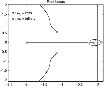
cannot be expressed in the form of D(s) þ KN(s) ¼ 0 with a single parameter K. Nevertheless, for each oowe can numerically calculate the roots of Equation (11.48) and plot them on the complex plane as oovaries within a range of interest. Figure 11.24 illustrates all the four branches, r1(K),. . .,r4(K), of the root locus for
−2 −1.5 −1 −0.5 0 0.5 1 1.5 2 −1.5 −1 −0.5 0 0.5 1 1.5 Real Axis Imag Axis
Root Locus for N(s) = s2+ s + 0.4, D(s) = s(s2− s − 0.4)
arrows show the increasing direction of K = 1/λ from 0 to +∞
FIGURE 11.23 The root locus with respect to K ¼ 1/l.
−2.5 −2 −1.5 −1 −0.5 0 −2 −1.5 −1 −0.5 0 0.5 1 1.5 2 Root Locus x : ωo= zero o : ωo= infinity
this system as ooincreases from zero to infinity. The figure is obtained by computing the roots of Equation (11.48) for a set of values of ooby using MATLAB.
Desired Pole Locations
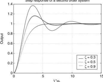
The performance of a feedback system depends heavily on the location of the closed-loop system poles ri(K) ¼ 1,. . .,n. First of all, for stability we want riðKÞ 2 C for all i ¼ 1,. . .,n. Clearly, having a pole ‘‘close’’ to the imaginary axis poses a danger, i.e., ‘‘small’’ perturbations in the plant might lead to an unstable feedback system. So the desired pole locations must be such that stability is preserved under such perturbations (or in the presence of uncertainties) in the plant. For second-order systems, we can define certain stability robustness measures in terms of the pole locations, which can be tied to the characteristics of the step response. For higher order systems, similar guidelines can be used by considering the dominant poles only.
In the standard feedback control system shown in Figure 11.22, assume that the closed-loop transfer function from r(t) to y(t) is in the form
TðsÞ ¼
s
2þ 2zo
o
2oo
s þ o
2o; 05z51; o
o2 R
and r(t) is the unit step function. Then, the output is
yðtÞ ¼ 1
e
ffiffiffiffiffiffiffiffi
zoot1 z
2p
sinðo
dt þ yÞ; t > 0
where od:¼ oo ffiffiffiffiffiffiffiffi 1 z2 pandy U cos–1(z). For some typical values of z, the step response y(t) is as shown in Figure 11.25. The maximum percent overshoot is defined to be the quantity
PO :¼
y
py
y
ssss
· 100%
where ypis the peak value. By simple calculations it can be seen that the peak value of y(t) occurs at the time
0 5 10 15 0 0.2 0.4 0.6 0.8 1 1.2 1.4 t*ωo Output
Step response of a second order system
ζ = 0.3 ζ = 0.5 ζ = 0.9
instant tp ¼ p/od, and
PO ¼ e
pz=p
ffiffiffiffiffi
1 z2· 100%
Figure 11.26 shows PO versus z. The settling time is defined to be the smallest time instant ts, after which the response y(t) remains within 2% of its final value, i.e.,
t
s:¼ min ft
0: yðtÞ y
ss< 0:02y
ss"t > t
0g
Sometimes 1% or 5% is used in the definition of settling time instead of 2%; conceptually, there is no difference. For the second-order system response, we have
t
s<
zo
4
oSo, in order to have a fast settling response, the product zooshould be large. The closed-loop system poles are
r
1;2¼ zo
o6 jo
offiffiffiffiffiffiffiffi
1 z
2q
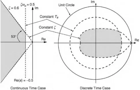
Therefore, once the maximum allowable settling time and PO are specified, we can define the region of desired pole locations by determining the minimum allowable z and zoo. For example, let the desired PO and tsbe bounded by
PO < 10% and t
s< 8s
The PO requirement implies that z $ 0.6, equivalentlyy # 53– (recall that cos(y) ¼ z). The settling time requirement is satisfied if and only if Re(r1,2) # –0.5. Then, the region of desired closed-loop poles is the shaded area shown in Figure 11.27. The same figure also illustrates the region of desired closed-loop poles for similar design requirements in the discrete time case.
0 0.1 0.2 0.3 0.4 0.5 0.6 0.7 0.8 0.9 1 0 10 20 30 40 50 60 70 80 90 100 ζ PO FIGURE 11.26 PO versus z.
If the order of the closed-loop transfer function T(s) is higher than two, then, depending on the location of its poles and zeros, it may be possible to approximate the closed-loop step response by the response of a second-order system. For example, consider the third-order system
TðsÞ ¼
ðs
2þ 2zo
o
2oo
s þ o
2oÞð1 þ s=rÞ
where r q zo
oThe transient response contains a term e–rt. Compared with the envelope e zoot of the sinusoidal term, e–rt
decays very fast, and the overall response is similar to the response of a second-order system. Hence, the effect of the third pole r3 ¼ –r is negligible.
Consider another example,
TðsÞ ¼
ðs
2þ 2zo
o
2o½1 þ s=ðr þ EÞ
o
s þ o
2oÞð1 þ s=rÞ
where 05E p r
In this case, although r does not need to be much larger than zoo, the zero at –(r þ E) cancels the effect of the pole at –r. To see this, consider the partial fraction expansion of Y(s) ¼ T(s)R(s) with R(s) ¼ 1/s:
YðsÞ ¼
A
s
0þ
s r
A
1 1þ
A
2s r
2þ
A
3s þ r
where A0 ¼ 1 andA
3¼ lim
s! rðs þ rÞYðsÞ ¼
o
2 o2zo
or ðo
2oþ r
2Þ
E
r þ E
Since Aj j ! 0 as E ! 0 the term A3 3e–rtis negligible in y(t).In summary, if there is an approximate pole–zero cancellation in the left half plane, then this pole–zero pair can be taken out of the transfer function T(s) to determine PO and ts. Also, the poles closest to the imaginary axis dominate the transient response of y(t). To generalize this observation, let r1,. . .,rnbe the poles of T(s), such that ReðrkÞ p Reðr2Þ ¼ Reðr1Þ50, for all k $ 3. Then, the pair of complex conjugate poles r1,2are called the dominant poles. We have seen that the desired transient response properties, e.g., PO and ts, can be translated into requirements on the location of the dominant poles.
Root Locus Construction
As mentioned above, the root locus primarily deals with finding the roots of a characteristic polynomial that is an affine function of a single parameter, K,
wðsÞ ¼ DðsÞ þ KNðsÞ
ð11:49Þ
where D(s) and N(s) are fixed monic polynomials (i.e., coefficient of the highest power is normalized to 1). If N and/or D are not monic, the highest coefficient(s) can be absorbed into K.
Root Locus Rules
Recall that the usual root locus shows the locations of the closed-loop system poles as K varies from 0 to þ 1. The roots of D(s), p1,. . .,pn, are the poles, and the roots of N(s), z1,. . .,zm, are the zeros, of the open-loop system, G(s) ¼ KF(s). Since P(s) and C(s) are proper, G(s) is proper, and hence n $ m. So the degree of the polynomial w(s) is n and it has exactly n roots.
Let the closed-loop system poles, i.e., roots of w(s), be denoted by r1(K),. . .,rn(K). Note that these are functions of K; whenever the dependence on K is clear, they are simply written as r1,. . .,rn. The points in C that satisfy (Equation (11.49)) for some K . 0 are on the root locus. Clearly, a point r 2 C is on the root locus if and only if
¼
FðrÞ
1
ð11:50Þ
The condition (Equation (11.50)) can be separated into two parts:
K
j j ¼
FðrÞ
1
j
j
ð11:51Þ
—K ¼ 0
–¼ ð2‘ þ 1Þ · 180
–—FðrÞ; ‘ ¼ 0; 61; 62; . . . :
ð11:52Þ
The phase rule (Equation (11.52)) determines the points in that are on the root locus. The magnitude rule (Equation (11.51)) determines the gain K . 0 for which the root locus is at a given point r. By using the definition of F(s), (Equation (11.52)) can be rewritten as
ð2‘ þ 1Þ · 180
–¼
X
n i¼1—ðr p
iÞ
X
m j¼1—ðr z
jÞ
ð11:53Þ
Similarly, (Equation (11.51)) is equivalent to
K ¼
Q
n i¼1r p
iQ
m j¼1r z
jð11:54Þ
Root Locus Construction
There are several software packages available for generating the root locus automatically for a given F ¼ N/D. In particular, the related MATLABcommands are rlocus and rlocfind. In many cases, approximate root
locus can be drawn by hand using the rules given below. These rules are determined from the basic definitions Equation (11.49), Equation (11.51), and Equation (11.52).
1. The root locus has n branches: r1(K),. . .,rn(K).
2. Each branch starts (K > 0) at a pole piand ends (as K ! 1) at a zero zj, or converges to an asymptote, Meja‘ where M ! 1) and
a
‘¼
2‘ þ 1
n m
· 180
–; ‘ ¼ 0; . . . ; ðn m 1Þ
3. There are (n – m) asymptotes with angles a‘. The center of the asymptotes (i.e., their intersection point on the real axis) is
s
a¼
P
ni¼1
P
iP
mj¼1z
jn m
4. A point x 2 R is on the root locus if and only if the total number of poles pi’s and zeros zj’s to the right of x (i.e., total number of pi’s with Re(pi) . x plus total number of zj’s with Re(zj) . x) is odd. Since F(s) is a rational function with real coefficients, poles and zeros appear in complex conjugates, so when counting the number of poles and zeros to the right of a point x 2 R we just need to consider the poles and zeros on the real axis.
5. The values of K for which the root locus crosses the imaginary axis can be determined from the Routh– Hurwitz stability test. Alternatively, we can set s ¼ jo in Equation (11.49) and solve for real o and K satisfying
Dð joÞ þ KNð joÞ ¼ 0
Note that there are two equations here, one for the real part and one for the imaginary part. 6. The break points (intersection of two branches on the real axis) are feasible solutions (satisfying rule 4)
of
d
ds
FðsÞ ¼ 0
ð11:55Þ
7. Angles of departure (K > 0) from a complex pole, or arrival K ! þ1 to a complex zero, can be determined from the phase rule. See example below.
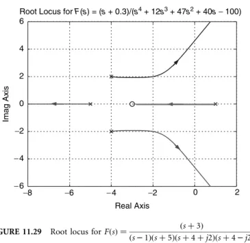
Let us now follow the above rules step by step to construct the root locus for
FðsÞ ¼
ðs þ 3Þ
ðs 1Þðs þ 5Þðs þ 4 þ j2Þðs þ 4 j2Þ
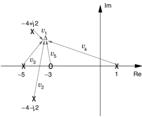
First, enumerate the poles and zeros as p1 ¼ –4 þ j2, p2 ¼ –4 – j2, p3 ¼ –5, p4 ¼ 1, z1 ¼ –3. So, n ¼ 4 and m ¼ 1.
1. The root locus has four branches.
2. Three branches converge to the asymptotes whose angles are 60–, 180–, and –60–, and one branch converges to z1 ¼ –3.
3. The center of the asymptotes iss ¼ (–12 þ 3)/3 ¼ –3. 4. The intervals (–1, –5] and [–3, 1] are on the root locus.
5. The imaginary axis crossings are the feasible roots of
ðo
4j12o
347o
2þ j40o 100Þ þ Kðjo þ 3Þ ¼ 0
ð11:56Þ
for real o and K. Real and imaginary parts of Equation (11.56) are
o
447o
2100 þ 3K ¼ 0
joð 12o
2þ 40 þ KÞ ¼ 0
They lead to two feasible pairs of solutions (K ¼ 100/3, o ¼ 0) and (K ¼ 215.83, o ¼ ^4.62). 6. Break points are the feasible solutions of
3s
4þ 36s
3þ 155s
2þ 282s þ 220 ¼ 0
Since the roots of this equation are –4.55 ^ j1.11 and –1.45 ^j1.11, there is no solution on the real axis, hence no break points.
7. To determine the angle of departure from the complex pole p1 ¼ –4 þ j2, let D represent a point on the root locus near the complex pole p1, and define vi, i ¼ 1,. . .,5, to be the vectors drawn from pi, for i ¼ 1,. . .,4, and from z1for i ¼ 5, as shown in Figure 11.28. Lety1,. . .,y5be the angles of v1,. . .,v5. The phase rule implies
ðy
1þ y
2þ y
3þ y
4Þ y
5¼ 6180
–ð11:57Þ
As D approaches p1,y1becomes the angle of departure and the otheryi’s can be approximated by the angles of the vectors drawn from the other poles, and from the zero, to the pole p1. Thusy1 can be solved from Equation (11.57), where y2 < 90–, y3 < tan–1(2), y4< 180– tan 1 25 , and y5< 90–þ tan1 12 . That yieldsy1< –15–.
The exact root locus for this example is shown in Figure 11.29. From the results of item 5 above, and the shape of the root locus, it is concluded that the feedback system is stable if
33:335K5215:83
Im Re −4+j2 −5 −3 5 4 1 −4−j2 2 3 ∆1i.e., by simply adjusting the gain of the controller, the system can be made stable. In some situations we need to use a dynamic controller to satisfy all the design requirements.
Design Examples Example 11.1
Consider the standard feedback system with a plant
PðsÞ ¼
1
0:72
1
ðs þ 1Þðs þ 2Þ
and design a controller such that. the feedback system is stable,
. PO # 10%, ts# 4 s, and steady state error is zero when r(t) is unit step, . steady state error is as small as possible when r(t) is unit ramp.
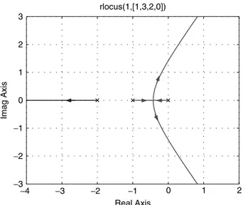
It is clear that the second design goal cannot be achieved by a simple proportional controller. To satisfy this condition, the controller must have a pole at s ¼ 0, i.e., it must have integral action. If we try an integral control of the form C(s) ¼ Kc/s, with Kc. 0, then the root locus has three branches, the interval [–1, 0] is on the root locus; three asymptotes have angles {60–, 180–, –60–} with a center ats
a ¼ –1, and there is only one break point at 1 þ 1ffiffi
3
p, see Figure 11.30. From the location of the break point, center, and angles of the asymptotes, it can be deduced that two branches (one starting at p1 ¼ –1, and the other one starting at p3 ¼ 0) always remain to the right of p1. On the other hand, the settling time condition implies that the real parts of the dominant closed-loop system poles must be less than or equal to –1. So, a simple integral control does not do the job. Now try a PI controller of the form
CðsÞ ¼ K
cs z
s
c; K
c40
−8 −6 −4 −2 0 2 −6 −4 −2 0 2 4 6 Real Axis Imag AxisRoot Locus for F(s) = (s + 0.3)/(s4+ 12s3+ 47s2+ 40s − 100)
In this case, we can select zc ¼ –1 to cancel the pole at p1 ¼ –1 and the system effectively becomes a second-order system. The root locus for F(s) ¼ 1/s(s þ 2) has two branches and two asymptotes, with center sa ¼ – 1 and angles {90–, –90–}; the break point is also at –1. The branches leave –2 and 0, and go toward each other, meet at –1, and tend to infinity along the line Re(s) ¼ –1. Indeed, the closed-loop system poles are
r
1;2¼ 1 6
ffiffiffiffiffiffiffi
1 K
p
; where K ¼ K
c=0:72
The steady state error, when r(t) is unit ramp, is 2/K. So K needs to be as large as possible to meet the third design condition. Clearly, Re(r1,2) ¼ –1 for all K $ 1, which satisfies the settling time requirement. The percent overshoot is less than 10% if z of the roots r1,2 is greater than 0.6. A simple algebra shows that z ¼ 1=pffiffiffiK, hence the design conditions are met if K ¼ 1/0.36, i.e. Kc ¼ 2. Thus a PI controller that solves the design problem is
CðsÞ ¼ 2
s þ 1
s
The controller cancels a stable pole (at s ¼ –1) of the plant. If there is a slight uncertainty in this pole location, perfect cancellation will not occur and the system will be third-order with the third pole at r3> –1. Since the zero at zo ¼ –1 will approximately cancel the effect of this pole, the response of this system will be close to the response of a second-order system. However, we must be careful if the pole–zero cancellations are near the imaginary axis because in this case small perturbations in the pole location might lead to large variations in the feedback system response, as illustrated with the next example.
Example 11.2
A flexible structure with lightly damped poles has transfer function in the form
PðsÞ ¼
o
21s
2ðs
2þ 2zo
1s þ o
21Þ
−1 −3 −2 −4 0 1 2 −3 −2 −1 0 1 2 3 Real Axis Imag Axis rlocus(1,[1,3,2,0])By using the root locus, we can see that the controller
CðsÞ ¼ K
cðs
2
þ 2zo
1
s þ o
21Þðs þ 0:4Þ
ðs þ rÞ
2ðs þ 4Þ
stabilizes the feedback system for sufficiently large r and an appropriate choice of Kc. For example, let o1 ¼ 2, z ¼ 0.1, and r ¼ 10. Then the root locus of F(s) ¼ P(s)C(s)/K, where K ¼ Kco21is as shown in Figure 11.31. For K ¼ 600, the closed-loop system poles are
f 10:78 6 j2:57; 0:94 6 j1:61; 0:2 6 j1:99; 0:56g
Since the poles –0.2 ^ j1.99 are canceled by a pair of zeros at the same point in the closed-loop system transfer function T ¼ G(1 þ G)–1, the dominant poles are at –0.56 and –0.94 ^ j1.61 (they have relatively large negative real parts and the damping ratio is about 0.5).
Now, suppose that this controller is fixed and the complex poles of the plant are slightly modified by taking z ¼ 0.09 and o1 ¼ 2.2. The root locus corresponding to this system is as shown in Figure 11.32. Since lightly damped complex poles are not perfectly canceled, there are two more branches near the imaginary axis. Moreover, for the same value of K ¼ 600, the closed-loop system poles are
f 10:78 6 j2:57; 1:21 6 j1:86; 0:05 6 j1:93; 0:51g
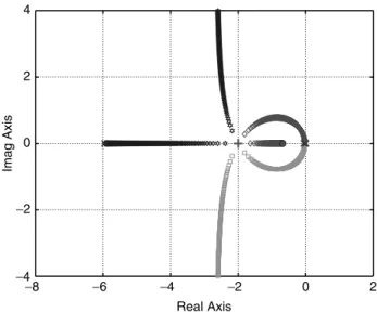
In this case, the feedback system is unstable.Example 11.3
One of the most important examples of mechatronic systems is the DC motor. An approximate transfer function of a DC motor [8, pp. 141–143] is in the form
P
mðsÞ ¼
sðs þ 1=t
K
m mÞ
; t
m40
−12 −10 −8 −6 −4 −2 0 2 4 −10 −8 −6 −4 −2 0 2 4 6 8 10 Real Axis Imag AxisAlso note that if tmis large, then Pm(s) < Pb(s), where Pb(s) ¼ Kb/s2, is the transfer function of a rigid beam. In this example, the general class of plants Pm(s) will be considered. Assuming that pm ¼ –1/tmand Kmare given, a first-order controller
CðsÞ ¼ K
cs p
s z
cc
ð11:58Þ
will be designed. The aim is to place the closed-loop system poles far from the Im-axis. Since the order of F(s) ¼ Pm(s)C(s)/KmKcis three, the root locus has three branches. Suppose the desired closed-loop poles are given as p1, p2, and p3. Then, the pole placement problem amounts to finding {Kc, zc, pc}such that the characteristic equation is
wðsÞ ¼ ðs p
1Þðs p
2Þðs p
3Þ ¼ s
3ðp
1þ p
2þ p
3Þs
2þ ðp
1p
2þ p
1p
3þ p
2p
3Þs p
1p
2p
3But the actual characteristic equation, in terms of the unknown controller parameters, is
wðsÞ ¼ sðs p
mÞðs p
cÞ þ kðs z
cÞ ¼ s
3ðp
mþ p
cÞs
2þ ðp
mp
cþ KÞs Kz
cwhere K : ¼ KmKc. Equating the coefficients of the desired w(s) to the coefficients of the actual w(s), three equations in three unknowns are obtained:
p
mþ p
c¼ p
1þ p
2þ p
3p
mp
cþ K ¼ p
1p
2þ p
1p
3þ p
2p
3Kz
c¼ p
1p
2p
3From the first equation pc is determined, then K is obtained from the second equation, and finally zc is computed from the third equation.
For different numerical values of pm, p1, p2, and p3the shape of the root locus is different. Below are some examples, with the corresponding root loci shown in Figure 11.33 to Figure 11.35.
−10 −8 −6 −4 −2 0 −4 −3 −2 −1 0 1 2 3 4 Real Axis Imag Axis
(a) pm¼ 0:05; p1¼ p2¼ p3¼ 2 )
K ¼ 11:70; p
c¼ 5:95; z
c¼ 0:68
(b) pm¼ 0:5; p1¼ 1; p2¼ 2; p3¼ 3 )K ¼ 8:25; p
c¼ 5:50; z
c¼ 0:73
(c) pm¼ 5; p1¼ 11; p2¼ 4 þ j1; p3¼ 4 j1)K ¼ 35; p
c¼ 14; z
c¼ 5:343
−8 −6 −4 −2 0 2 −4 −2 0 2 4 Real Axis Imag AxisFIGURE 11.33 Root locus for Example 11.3(a).
−6 −5 −4 −3 −2 −1 0 1 −4 −3 −2 −1 0 1 2 3 4 Real Axis Imag Axis
Example 11.4
Consider the open-loop transfer function
PðsÞCðsÞ ¼ K
cðs
2
3s þ 3Þðs z
cÞ
sðs
2þ 3s þ 3Þðs p
cÞ
where Kcis the controller gain to be adjusted, and zcand pc are the controller zero and pole, respectively. Observe that the root locus has four branches except for the non-generic case zc ¼ pc. Let the desired dominant closed-loop poles be r1,2 ¼ –0.4. The steady state error for unit ramp reference input is
e
ss¼
K
p
c cz
cAccordingly, we want to make the ratio Kczc/pcas large as possible. The characteristic equation is
wðsÞ ¼ sðs
2þ 3s þ 3Þðs p
cÞ þ K
cðs
23s þ 3Þðs z
cÞ
and it is desired to be in the form
wðsÞ ¼ ðs þ 0:4Þ
2ðs r
3Þðs r
4Þ
for some r3,4with Re(r3,4) , 0, which implies that
wðsÞj
s¼ 0:4¼ 0;
ds
d
wðsÞj
s¼ 0:4¼ 0
ð11:59Þ
Conditions (Equation (11.59)) give two equations:
0:784ð0:4 þ p
cÞ 4:36K
cð0:4 þ z
cÞ ¼ 0
−16 −14 −12 −10 −8 −6 −4 −2 0 2 −6 −4 −2 0 2 4 6 Real Axis Imag Axis4:36K
c0:784 1:08ð0:4 þ p
cÞ þ 3:8K
cð0:4 þ z
cÞ ¼ 0
from which zcand pccan be solved in terms of Kc. Then, by simple substitutions, the ratio to be maximized, Kczc/pc,can be reduced to
K
cz
cp
c¼
3:4776K
c0:784
24:2469K
c3:4776
The maximizing value of Kc is 0.1297; it leads to pc ¼ –0.9508 and zc ¼ –1.1637. For this controller, the feedback system poles are
f 1:64 þ j0:37; 1:64 j0:37; 0:40; 0:40g
The root locus is shown in Figure 11.36.11.4
Complementary Root Locus
In the previous section, the root locus parameter K was assumed to be positive and the phase and magnitude rules were established based on this assumption. There are some situations in which controller gain can be negative as well. Therefore, the complete picture is obtained by drawing the usual root locus (for K . 0) and the complementary root locus (for K , 0). The complementary root locus rules are
‘ · 360
–¼
X
n i¼1—ðr p
iÞ
X
n j¼1—ðr z
jÞ; ‘ ¼ 0; 61; 62; . . .
ð11:60Þ
jKj ¼
P
ni¼1r p
ij
P
m j¼1r z
jð11:61Þ
Since the phase rule (Equation (11.60)) is the 180–shifted version of (Equation (11.53)), the complementary root locus is obtained by simple modifications in the root locus construction rules. In particular, the number−3 −2 −1 0 1 2 −1.5 −1 −0.5 0 0.5 1 1.5 Real Axis Imag Axis
of asymptotes and their center are the same, but their angles a‘’s are given by
a
‘¼
ðn mÞ
2‘
· 180
–; ‘ ¼ 0; . . . ; ðn m 1Þ
Also, an interval on the real axis is on the complementary root locus if and only if it is not on the usual root locus.
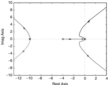
Example 11.3 (revisited)
In the Example 11.3 given above, if the problem data is modified to pm ¼ –5, p1 ¼ –20, and p2,3 ¼ –2 ^ j, then the controller parameters become
K ¼ 10; p
c¼ 19; z
c¼ 10
Note that the gain is negative. The roots of the characteristic equation as K varies between 0 and –1 form the complementary root locus; see Figure 11.37.
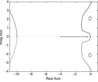
Example 11.4 (revisited)
In this example, if K increases from –1 to þ1, the closed-loop system poles move along the complementary root locus, and then the usual root locus, as illustrated in Figure 11.38.
11.5
Root Locus for Systems with Time Delays
The standard feedback control system considered in this section is shown in Figure 11.39, where the controller C and plant P are in the form
CðsÞ ¼
N
D
cðsÞ
cðsÞ
−25 −20 −15 −10 −5 0 5 10 15 20 25 −10 −8 −6 −4 −2 0 2 4 6 8 10 Real Axis Imag AxisComplementary Root Locus arrows indicate
increasing direction of K from ∞ to 0
and
PðsÞ ¼ e
hsP
0
ðsÞ where P
0ðsÞ ¼
N
D
pðsÞ
pðsÞ
with (Nc, Dc) and (Np, Dp) being coprime pairs of polynomials with real coefficients.1The term e–hsis the transfer function of a pure delay element (in Figure 11.39 the plant input is delayed by h seconds). In general, time delays enter into the plant model when there is
. a sensor (or actuator) processing delay, and/or . a software delay in the controller, and/or . a transport delay in the process.
In this case the open-loop transfer function is
GðsÞ ¼ G
hðsÞ ¼ e
hsG
0ðsÞ
where G0(s) ¼ P0(s)C(s) corresponds to the no delay case, h ¼ 0.
−4 −2 0 2 4 6 8 −5 −4 −3 −2 −1 0 1 2 3 4 5 Real Axis Imag Axis
Complete Root Locus for −∞ < K < +∞
FIGURE 11.38 Complementary and usual root loci for Example 11.4.
1A pair of polynomials is said to be coprime pair if they do not have common roots
+ P 0(s) u(t-h) y(t) v(t) −+ u(t) e−hs − P(s) C(s) r(t) e(t)
Note that magnitude and phase of G(jo) are determined from the identities
Gð joÞ ¼ G
0ð joÞj
ð11:62Þ
—Gð joÞ ¼ ho þ —G
0ð joÞ
ð11:63Þ
Stability of Delay Systems
Stability of the feedback system shown in Figure 11.39 is equivalent to having all the roots of
wðsÞ ¼ DðsÞ þ e
hsNðsÞ
ð11:64Þ
in the open left half plane, C , where D(s) ¼ Dc(s)Dp(s) and N(s) ¼ Nc(s)Np(s). We assume that there is no unstable pole–zero cancellation in taking the product P0(s)C(s), and that deg(D) . deg(N) (here N and D need not be monic polynomials). Strictly speaking, w(s) is not a polynomial because it is a transcendental function of s. The functions of the form (Equation (11.64)) belong to a special class of functions called quasi-polynomials. The closed-loop system poles are the roots of (Equation (11.64)).
Following are known facts (see [1,10]):
(i) If rkis a root of Equation (20), then so is rrk. (i.e., roots appear in complex conjugate pairs as usual) (ii) There are infinitely many poles rk2 C; k ¼ 1, 2,. . ., satisfying w(rk) ¼ 0.
(iii) And rk’s can be enumerated in such a way that Re(rkþ 1) # Re(rk) moreover, Re(rk) ! –1 as k!1. Example 11.5
If Gh(s) ¼ e–hs/s, then the closed-loop system poles rk, for k ¼ 1, 2,. . ., are the roots of
1 þ
e
s
hske
jhokk
þ jo
ke
6j2kp
¼ 0
ð11:65Þ
where rk ¼ sk þ jokfor some sk; ok2 R Note that e^j2kp ¼ 1 for all k ¼ 1, 2,. . .. Equation (11.45) is equivalent to the following set of equations:
e
hsk¼ s
k
þ jo
kj
ð11:66Þ
6ð2k 1Þp ¼ ho
kþ —ðs
kþ jo
kÞ; k ¼ 1; 2; . . .
ð11:67Þ
It is quite interesting that for h ¼ 0 there is only one root r ¼ –1, but even for infinitesimally small h . 0 there are infinitely many roots. From the magnitude condition (Equation (11.66)), it can be shown that
s
k> 0 ) o
j
kj
< 1
ð11:68Þ
Also, forsk$ 0 the phase /(skþ jok) is between –p/2 and þp/2, therefore Equation (11.67) leads to
s
k> 0 ) h o
j j>
kp
2
ð11:69Þ
By combining Equation (11.68) and Equation (11.69), it can be proven that the feedback system has no roots in the closed right half plane when h , p/2. Furthermore, the system is unstable if h $ p/2. In particular, for h ¼ p/2 there are two roots on the imaginary axis, at ^j1. It is also easy to show that, for any h . 0 as k ! 1, the roots converge to
r
k!
1
h
ln
2kp
h
6 j2kp
As h ! 0, the magnitude of the roots converge to 1.
As illustrated by the above example, property (iii) implies that for any given real numbers there are only finitely many rk’s in the region of the complex plane
C
s:¼ fs 2 C : ReðsÞ > sg
In particular, withs ¼ 0, this means that the quasi-polynomial w(s) can have only finitely many roots in the right half plane. Since the effect of the closed-loop system poles that have very large negative real parts is negligible (as far as closed-loop systems’ input–output behavior is concerned), only finitely many ‘‘dominant’’ roots rk, for k ¼ 1,. . .,m, should be computed for all practical purposes.
Dominant Roots of a Quasi-Polynomial
Now we discuss the following problem: given N(s), D(s), and h $ 0, find the dominant roots of the quasi-polynomial
wðsÞ ¼ DðsÞ þ e
hsNðsÞ
For each fixed h . 0, it can be shown that there existssmaxsuch that w(s) has no roots in the region, Csmax; see
[11] for a simple algorithm to estimatesmax, based on Nyquist criterion. Given h . 0 and a region of the complex plane defined bysmin# Re(s) #smax, the problem is to find the roots of w(s) in this region.
Clearly, a point r ¼ s þ jo in C is a root of w(s) if and only if
Dðs þ joÞ ¼ e
hse
jhoNðs þ joÞ
Taking the magnitude square of both sides of the above equation, w(r) ¼ 0 implies
A
sðxÞ :¼ Dðs þ xÞDðs xÞ e
2hsNðs þ xÞNðs xÞ ¼ 0
where x ¼ jo. The term D(s þ x) stands for the function D(s) evaluated at s þ x. The other terms of As(x) are calculated similarly. For each fixeds, the function As(x) is a polynomial in the variable x. By symmetry, if x is a zero of As(·) then (–x) is also a zero.
If As(x) has a root x‘whose real part is zero, set r‘¼ s þ x‘. Next, evaluate the magnitude of wðr‘Þ; if it is zero, then n‘is a root of w(s). Conversely, if As(x) has no root on the imaginary axis, then w(s) cannot have a root whose real part is the fixed value ofs from which As(·) is constructed.
Algorithm
Given N(s), D(s), h,smin, andsmax:
Step 1. Picks values s1,. . .,sMbetweensminandsmaxsuch thatsmin ¼ s1,si,siþ1, andsM¼ smax. For eachsiperform the following.
Step 2. Construct the polynomial Ai(x) according to
A
iðxÞ :¼ Dðs
iþ xÞDðs
ixÞ e
2hsiNðs
iþ xÞNðs
ixÞ
Step 3. For each imaginary axis roots x‘of Ai, perform the following test:
Check if jwðsiþ x‘Þj ¼ 0; if yes, then r ¼ siþ x‘ is a root of w(s); if not, discard x‘. Step 4. If i ¼ M, stop; else increase i by 1 and go to Step 2.
Example 11.6
We will find the dominant roots of
1 þ
e
s
hs¼ 0
ð11:70Þ
for a set of critical values of h. Recall that Equation (11.70) has a pair of roots ^j1 when h ¼ p/2 ¼ 1.57. Moreover, dominant roots of Equation (11.70) are in the right half plane if h . 1.57, and they are in the left half plane if h , 1.57. So, it is expected that for h [ (1.2, 2.0) the dominant roots are near the imaginary axis. Takesmin ¼ –0.5 andsmax ¼ 0.5, with M ¼ 400 linearly spacedsi’s between them. In this case
A
iðxÞ ¼ s
2ie
2hsix
2Whenever e 2hsi> s2
i; AiðxÞ has two roots:
x
‘¼ 6j
ffiffiffiffiffiffiffiffiffiffiffiffiffi
e
2hsis
2 iq
; ‘ ¼ 1; 2
For each fixedsisatisfying this condition, let r‘¼ siþ x‘(note that x‘is a function ofsi, so r‘is a function ofsi) and evaluate
f ðs
iÞ :¼ 1 þ
e
hr‘r
‘If f(si) ¼ 0, then x‘ is a root of 11.70. For 10 different values of h [ (1.2, 2.0), the function f (s) is plotted in Figure 11.40. This figure shows the feasible values ofsifor which x‘ (defined fromsi) is a root of Equation (11.70). The dominant roots of Equation (11.70), as h varies from 1.2 to 2.0, are shown in Figure 11.41. For h , 1.57, all the roots are in C : For h . 1.57, the dominant roots are in Cþ;,and for h ¼ 1.57, they are at ^j1.
Root Locus Using Pade´ Approximations
In this section we assume that h . 0 is fixed and we try to obtain the root locus, with respect to uncertain/ adjustable gain K, corresponding to the dominant poles. The problem can be solved by numerically calculating
−0.4 −0.3 −0.2 −0.1 0 0.1 0.2 0.3 10−2 10−1 100 101 σ
Detection of the Roots
h = 1.2 h = 2.0
h = 1.29
f(
σ)
the dominant roots of the quasi-polynomial
wðsÞ ¼ DðsÞ þ KNðsÞe
hsð11:71Þ
for varying K, by using the methods presented in the previous section. In this section an alternative method is given that uses Pade´ approximation of the time delay term e–hs. More precisely, the idea is to find polynomials Nh(s) and Dh(s) satisfying
e
hs<
N
D
hðsÞ
h
ðsÞ
ð11:72Þ
so that the dominant roots
DðsÞD
hðsÞ þ KNðsÞN
hðsÞ ¼ 0
ð11:73Þ
closely match the dominant roots of w(s), (11.71). How should we do the approximation (Equation (11.72)) for this match?
By using the stability robustness measures determined from the Nyquist stability criterion, we can show that for our purpose we may consider the following cost function in order to define a meaningful measure for the approximation error:
D
h¼: sup
ok
maxNðjoÞ
DðjoÞ
e
jhoN
hðjoÞ
D
hðjoÞ
where Kmaxis the maximum value of interest for the uncertain/adjustable parameter K. The ‘ th order Pade´ approximation is defined as follows:
N
hðsÞ ¼
X
‘ k¼0ð 1Þ
kc
kh
ks
kD
hðsÞ ¼
X
‘ k¼0c
kh
ks
k −0.2 −0.1 0 0.1 −1.5 −1 −0.5 0 0.5 11.5 Locus of dominant roots for 1.2 < h < 2.0
h = 1.2 h = 1.2 h = 2.0 h = 2.0 h = π/2 h = π/2
where coefficients ck’s are computed from
c
k¼
2‘!k!ð‘ kÞ!
ð2‘ kÞ!‘!
; k ¼ 0; 1; . . . ; ‘
First-and second-order approximations are in the form
N
hðsÞ
D
hðsÞ
¼
1 hs=2
1 þ hs=2 ;
‘ ¼ 1
1 hs=2 þ ðhsÞ
2=12
1 þ hs=2 þ ðhsÞ
2=12
; ‘ ¼ 2
8
>
>
<
>
>
:
Given the problem data {h, Kmax, N(s), D(s)}, how do we find the smallest degree, ‘, of the Pade´ approximation, so that Dh # d (or Dh/Kmax# d0) for a specified error d, or a specified relative error d0? The answer lies in the following result [7]: for a given degree of approximation ‘ we have
e
jhoN
D
hð joÞ
hð joÞ
<
2
eho
4‘
2‘þ1; o <
4‘
eh
2;
o >
4‘
eh
8
>
>
<
>
>
:
In light of this result, we can solve the approximation order selection problem by using the following procedure:
1. Determine the frequency oxsuch that
K
maxNð joÞ
Dð joÞ
<
d
2
; for all o > o
x and initialize ‘ ¼ 1:2. For each ‘ > 1 define
o
‘¼ max o
X;
4‘
eh
:
and plot the function
F
‘ðoÞ :¼
2
K
maxDð joÞ
Nð joÞ
eho
4‘
2‘þ1; for o <
4‘
eh
2
K
maxDð joÞ
Nð joÞ
;
for o
‘> o >
4‘
eh
8
>
>
<
>
>
:
3. Check Ifmax
o2½0;oxF
‘ðoÞ < d
ð11:74Þ
If yes, stop, this value of ‘ satisfies the desired error bound: Dh# d. Otherwise, increase ‘ by 1, and go to Step 2. Note that the left-hand side of the inequality (Equation (11.74)) is an upper bound of Dh. Since we assumed deg(D) . deg(N), the algorithm will pass Step 3 eventually for some finite ‘ > 1: At each iteration, we have to draw the error function F‘ðoÞ and check whether its peak value is less than d. Typically, as d decreases, oxincreases, and that forces ‘ to increase. On the other hand, for very large values of ‘, the relative magnitude c0=c‘ of the coefficients becomes very large, in which case numerical difficulties arise in analysis and simulations. Also, as time delay h increases, ‘ should be increased to keep the level of the approximation error d fixed. This is a fundamental difficulty associated with time delay systems.
Example 11.7
Let N(s) ¼ s þ1, D(s) ¼ s2þ2sþ2 and h ¼ 0.1, and K
max ¼ 20. Then, for d0 ¼ 0.05 applying the above procedure we calculate ‘ ¼ 2 as the smallest approximation degree satisfying Dh/Kmax,d0. Therefore, a second-order approximation of the time delay should be sufficient for predicting the dominant poles for K [ [0, 20]. Figure 11.42 shows the approximate root loci obtained from Pade´ approximations of degrees‘ ¼ 1; 2; 3: There is a significant difference between the root loci for ‘ ¼ 1 and ‘ ¼ 2: In the region Re(s) $ –12, the predicted dominant roots are approximately the same for ‘ ¼ 2; 3, for K[[0,20]. So, we can safely say that using higher order approximations will not make any significant difference as far as predicting the behavior of the dominant poles for the given range of K.
Notes and References
This section in the chapter is an edited version of related parts of the author’s book [9]. More detailed discussions of the root locus method can be found in all the classical control books, such as [2, 5, 6, 8]. As mentioned earlier, extension of this method to discrete time systems is rather trivial: the method to find the roots of a polynomial as a function of a varying real parameter is independent of the variable s (in the continuous time case) or z (in the discrete time case). The only difference between these two cases is the definition of the desired region of the complex plane: for the continuous time systems, this is defined relative to the imaginary axis, whereas for the discrete time systems the region is defined with respect to the unit circle, as illustrated in Figure 11.27.
References
1. Bellman, R.E., and Cooke, K.L., Differential Difference Equations, Academic Press, New York, 1963. 2. Dorf, R.C., and Bishop, R.H., Modern Control Systems, 9th ed., Prentice-Hall, Upper Saddle River, NJ, 2001. 3. Evans, W.R., ‘‘Graphical analysis of control systems,’’ Transac. Amer. Inst. Electrical Engineers, vol. 67 (1948),
pp. 547–551.
4. Evans, W.R., ‘‘Control system synthesis by root locus method,’’ Transac. Amer. Inst. Electrical Engineers, vol. 69 (1950), pp. 66–69.
5. Franklin, G.F., Powell, J.D., and Emami-Naeini, A., Feedback Control of Dynamic Systems, 3rd ed., Addison Wesley, Reading, MA, 1994.
−12 −10 −8 −6 −4 −2 0 2 −25 −20 −15 −10 −5 0 5 10 15 20
25Root Loci with Pade Approximations of Orders 1, 2, and 3
l = 2 l = 3
l = 1 K = 20.6
K = 16.1
6. Kuo, B.C., Automatic Control Systems, 7th ed., Prentice-Hall, Upper Saddle River, NJ, 1995.
7. Lam, J., ‘‘Convergence of a class of Pade´ approximations for delay systems,’’ Int. J. Control, vol. 52 (1990), pp. 989–1008.
8. Ogata, K., Modern Control Engineering, 3rd ed., Prentice-Hall, Upper Saddle River, NJ, 1997. 9. O¨zbay, H., Introduction to Feedback Control Theory, CRC Press LLC, Boca Raton, FL, 2000.
10. Stepan, G., Retarded Dynamical Systems: Stability and Characteristic Functions, Longman Scientific & Technical, New York, 1989.
11. Ulus, C., ‘‘Numerical computation of inner-outer factors for a class of retarded delay systems,’’ Int. J. Systems Sci., vol. 28 (1997), pp. 897–904.
11.5
Compensation
Charles L. Phillips and Royce D. Harbor
Compensation is the process of modifying a closed-loop control system (usually by adding a compensator or controller) in such a way that the compensated system satisfies a given set of design specifications. This section presents the fundamentals of compensator design; actual techniques are available in the references.
A single-loop control system is shown in Figure 11.43. This system has the transfer function from input R(s) to output C(s)
TðsÞ ¼
CðsÞ
RðsÞ
¼
G
cðsÞG
pðsÞ
1 þ G
cðsÞG
pðsÞHðsÞ
ð11:75Þ
and the characteristic equation is
1 þ G
cðsÞG
pðsÞHðsÞ ¼ 0
ð11:76Þ
where Gc(s) is the compensator transfer function, Gp(s) is the plant transfer function, and H(s) is the sensor transfer function. The transfer function from the disturbance input D(s) to the output is Gd(s)/ [1 þ Gc(s)Gp(s)H(s)]. The function Gc(s)Gp(s)H(s) is called the open-loop function.
FIGURE 11.43 A closed-loop control system. (Source: C.L. Phillips and R.D. Harbor, Feedback Control Systems, 2nd ed., Englewood Cliffs, N.J.: Prentice-Hall, 1991, p. 161. With permission.)