Parallel maze routing algorithms on a hypercube multicomputer

,G':Ö.R1THI^S'·' QM

é

A : r í t a l a ,

■ёУ'іі'';ѵ1'ГДі"±£'·· T H i¿ f 4^r'CO'ÍVi'-’'.-UvI£'K iv í’«-·; .·■ ; -Ef'-iя ■f.*i ·'„ті.f '".!···)■ i;C4...úr-'s ■.

i· J... V .»1«*»^: ¿;S»t M ir · ’•«V^ J l i -j l í ' Й *· 5 i «i ‘ЦЙГ? ■ «W il ..w . гЛ-" «i;4

ϊέ ίω TK-i Jf< íj'nrüT?.

0

? íi4íGí;.';£?fii/-ie Ä «ö:,S C ilj. .■■, .■ r e í i'.·: v7jjT.'vjSiira'S4S.}b!T./· V . * / - ··»,-’ — . ^ w - .. - . ., X , « j 1. ^ ■ .y * -- / ^ : Ίί’^· ■r». _ «*· ,r-;i , ^e.*> к«л; .,■•1 !· t r:,..1 í f " r : j m m • . j v . ^ s V r r , j í l; ••^· ·. ■«· . — v ^ / / ' V , X r ■ L r . , : < · ' ‘. X ' ' é ' ' i - ir ‘' -.. / f ^ .*; >··\ и ; . г / г .-u, ,J r r .· . ■ · : '·■· ■ ■ · ·■ ; ; , >»ь;.,- ' j• ?*N. _■χιτ• ...

PARALLEL MAZE ROUTING ALGORITHMS ON A

HYPERGUBE MULTICOMPUTER

A THESIS

SUBMITTED TO THE DEPARTMENT OF COMPUTER ENGINEERING AND INFORMATION SCIENCE AND THE INSTITUTE OF ENGINEERING AND SCIENCE

OF BILKENT UNIVERSITY

IN PARTIAL FULFILLMENT OF THE REQUIREMENTS FOR THE DEGREE OF

MASTER OF SCIENCE

By

Tahsin Mertefe Kurg

November 1991

i> . 3 5 6 5 t

n

I certify that I have read this thesis and th at in my opin­ ion it is fully adequate, in scope and in quality, as a thesis for the degree of Master of Scienc^.

s

Assoc. Prof. Dr. Cevdet Aykanat (Principal Advisor)

I certify that I have read this thesis and that in my opin­ ion it is fully adequate, in scope and in quality, as ajiiesis for the degree of Master of Science.

r. Kemal Oflazer

I certify that I have read this thesis and that in my opin­ ion it is fully adequate, in scope and in quality, as a thesis for the degree of Master of Science.

Prof. Dr. Mehmet Baray

Approved by the Institute of Engineering and Science;

ABSTRACT

PARALLEL MAZE ROUTING ALGORITHMS ON A

HYPERCUBE MULTICOMPUTER

Talisin Mertefe Kurg

M. S. in Computer Engineering and Information Science

Supervisor: Assoc. Prof. Dr. Cevdet Aykanat

November, 1991

Global routing phase is a time consuming task in VLSI layout. In global routing phase of the layout problem, the overall objective is to realize all the net interconnections using shortest paths. Efficient heuristics are used for the global routing phase. However, clue to the assumptions and constraints they impose, heuristics may fail to find a path for a net even if one exists. Re-routing is required for such nets. This re-routing phase requires the exhaustive search of the wiring area. Lee’s maze routing algorithm and Lee type maze routing algorithms are exhaustive search algorithms used in re-routing phase.

These algorithms are computationally expensive algorithms and consume large amounts of computer time for large grid sizes. Hence, these algorithms are good candidates for parallelization. Also, these algorithms require large memory space to hold the wiring grid. Therefore, the effective paralleliza­ tion of these algorithms require the partitioning of the computations and the grid among the processors. Hence, these algorithms can be parallelized on distributed-memory message passing multiprocessors (multicomputers).

IV

In this work, efficient parallel Lee type maze routing algorithms are devel­ oped for hypercube-connected multi computers. These algorithms are imple­ m ented on an Intel’s iPSC/2 hypercube multicomputer.

Keywords: VLSI layout, maze routing, Lee’s maze routing algorithm, Lee type maze routing algorithms, multicomputer, hypercube topology.

ÖZET

HİPERKUP ÇOK

i ş l e m c i l i

BİLGİSAYARINDA PARALEL

LABİRENT YOL BELİRLEME ALGORİTMALARI

Tahsin Mertefe Kıırç

Bilgisayar Mühendisliği ve Enformatik Bilimleri Bölümü

Yüksek Lisans

Tez Yöneticisi: Doçent Dr. Cevdet Aykanat

Kasım, 1991

Tümdevre tasarımında, devre bağlantılarının yapılması zaman alan bir iştir. Burada amaç bütün devre bağlantılarını en kısa yolları kullanarak yapmaktır. Eğer, her seferinde bir devre grubunun bağlantısı yapılırsa bunun adına labirent yol belirleme yöntemi denir.

Bu yöntem için, hüristik algoritmalar vardır. Ancak, bu tip algoritmalar de­ vre bağlantılarına getirdikleri kısıtlamalardan dolayı, bazen var olan bağlantıları bulamazlar. Bu yüzden, devrelerin bulunduğu alanın, tümden taranması gereke­ bilir. Lee’nin algoritması ve Lee benzeri algoritmalar bu tip algoritmalardır.

Lee’nin algoritması ve Lee benzeri algoritmalar hesaplama bakımından jja- halı ve devre yüzeyi için çok bilgisa5'^ar hafızası gerektiren algoritmalardır. Bu nedenle bu tip algoritmalar çok işlemcili bilgisayarlarda, paralel olarak çözmek için uygundur.

Bu çalışmada, Lee benzeri labirent }ml bulma algoritmalarının, hiperküp çok işlemcili bilgisayarında paralelleştirilmesi anlatılmaktadır.

VI

Anahtar kelimeler: Tûmdevre tasarımı, labirent yol bulma yöntemi, Lee’nin labirent 3ml bulma algoritması, Lee benzeri labirent algoritmaları, çok işlemcili bilgisayar, hiperküp topolojisi.

ACKNOWLEDGEMENT

I wish to thank very much my supervisor Assoc. Prof. Dr. Cevdet .Aykanat, who has guided and encouraged me during the development of this thesis.

I am grateful to Professor Mehmet Baray and Assoc. Prof. Dr. Kemal Oflazer for their remarks and comments on the thesis.

It is pleasure to express my thanks to all my friends for their valuable discussions and to my family for providing morale support during this studjL

Contents

1 INTRODUCTION 1

2 SEQUENTIAL MAZE ROUTING ALGORITHMS 10

2.1 Lee’s Maze Routing A lgorithm ... 10

2.2 Lee Type Algorithms For Routing of Multipin N e t s ... 13

2.2.1 Using Prim ’s A lg o r ith m ... 17

2.2.2 Using Kruskal’s A lg o rith m ... 18

3 PARALLELIZATION OF LEE’S ALGORITHM 23 3.1 Grid Partitioning and M a p p i n g ... 24

3.2 Parallel Front Wave Expansion ... 29

3.2.1 Expansion Starting From Source Only 29 3.2.2 Expansion Starting From Source and T a r g e t ... 35

3.3 Termination D e te c tio n ... 42

3.3.1 Global Synchronization 42 3.3.2 Counter Termination S c h e m e l... 43

3.3.3 Counter Termination S chem e2... 43

3.4 Overlapping Communication with C o m p u ta tio n ... 46

3.5 Asynchronous Scheme 49

3.5.1 Expansion Starting From Source Only 49 3.5.2 Expansion Starting From Source and Target 51 3.6 Parallel Path Recovery and Sw eeping... 55

3.6.1 Non-pipelined scheme... 57 3.6.2 Pipelined S ch em e... 57

3.7 Experimental Results 63

4 PARALLEL ALGORITHMS FOR MULTIPIN NETS 72

4.1 Parallel Akers’ Algorithm for Multipin Nets 72 4.2 Parallel Kruskal’s Steiner Tree A lgorithm ... 74 4.3 Experimental R e su lts... 77

5 CONCLUSIONS 84

List of Figures

1.1 Grid representation of the wiring surface in gate array layout. 3 1.2 (a) Single bend path (heuristic can find such a path) (b)

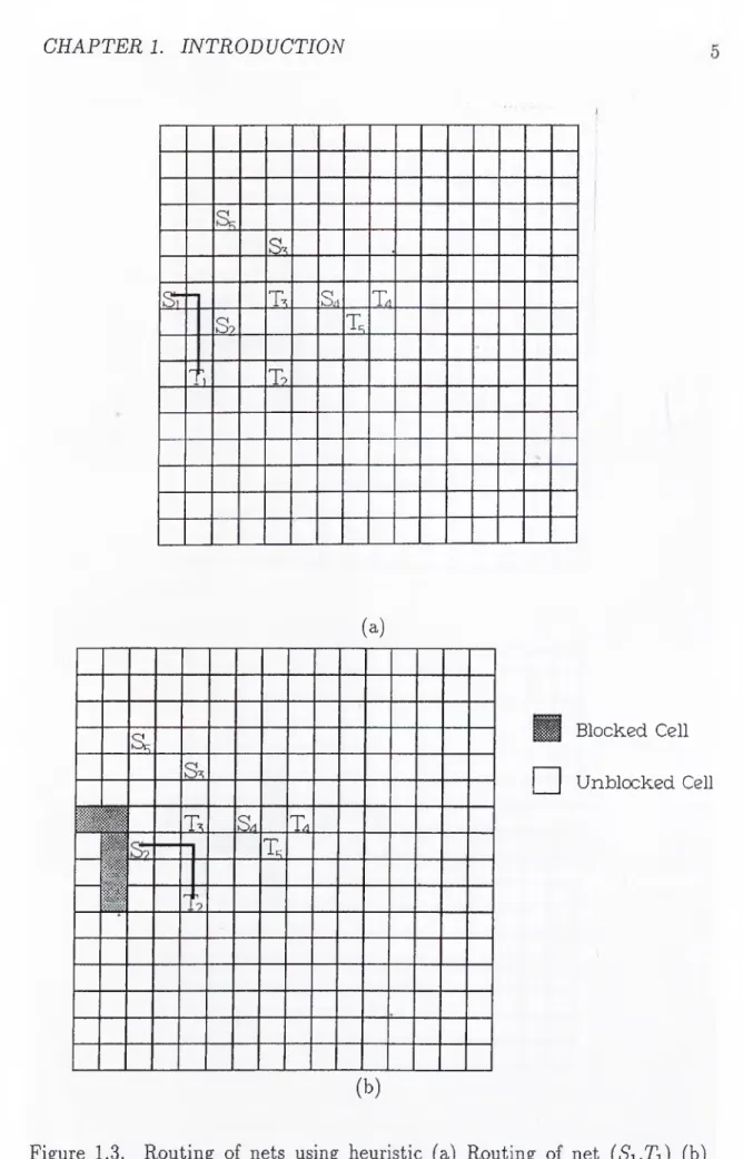
Two-bend path (heuristic fails to find such a p ath )... 4 1.3 Routing of nets using heuristic (a) Routing of net (,Si,Ti) (b)

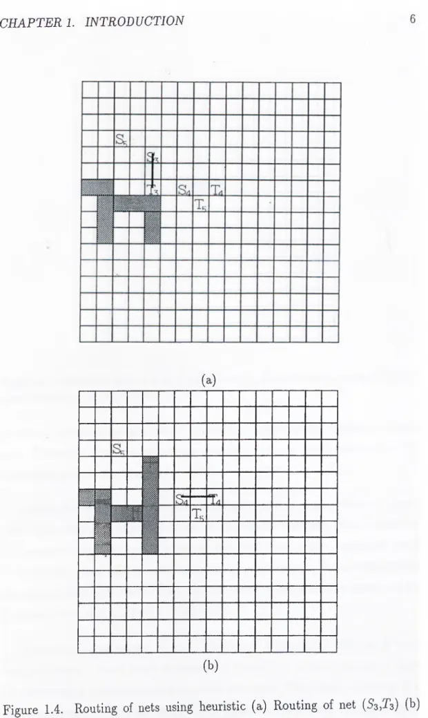
Routing of net (5’2,T2)... 5 1.4 Routing of nets using heuristic (a) Routing of net (SajTa) (b)

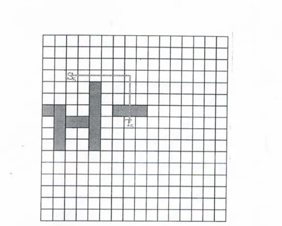
Routing of net (34^X4)... 6 1.5 Heuristic fails to find the path for (S'sjTs), because the path

(dotted lines) violates cell capacities. 7 1.6 8 node hypercube structure 8

2.1 A sample global grid for Lee’s maze routing algorithm ... 11 2.2 Front wave expansion phase of the Lee’s maze routing algorithm 11 2.3 Path recovery phase of the Lee’s maze routing ¿ilgorithm 12 2.4 Sweeping phase of the Lee’s maze routing alg o rith m ... 13 2.5 Front wave expansion phase of the Lee’s algorithm (a) Initial

cycles of front wave expansion phase (b) Successful termination of front wave expansion... 14

2.6 Path recovery and sweep phases of Lee’s algorithm after the front wave expansion phase (a) Path Recovery phase (b) Final configuration after sweep p h a s e ... 15 2.7 The use of the sweep queue, cells marked as 1,2,3 are added into

the sweep queue at expansion cj^cles 3,3, and 2, respectively. . . 16 2.8 Sequential version of the algorithm for routing multipin nets

using Prim ’s a lg o rith m ... 18 2.9 Front wave expansion phase of the Akers’ algorithm beginning

from the terminal cell ’a ’ (a) initial two cycles (b) Initial cycle after the first path (a to b) is connected... 19 2.10 The final configuration after all three pins are connected . . . . 20 2.11 Sequential version of the algorithm for routing multipin nets

using Kruskal’s algorithm 21

2.12 Routing of a three pin net using Kruskal’s algorithm (a) Initial cycles of the algorithm (b) After connecting all p i n s ... 22

3.1 Mesh embedding (a) hypercube of dimension 2 (b) h}q5ercube of dimension 3 (c) hypercube of dimension 4 25 3.2 Tiled decomposition of a 16x16 grid onto 2x4 mesh embedded

3-dimensional h y p e rc u b e ... 26 3.3 Scattered decomposition of a 16x16 grid 28 3.4 Decomposition of 16x16 grid into subblocks of (a) h = w = 2

(b) h = 2w = 4 ... 30 3.5 Local data structures for a node processor... 31 3.6 Node program for the Sonly scheme 32 3.7 Encoding the status inform ation... 33

3.8 Mapping of local coordinates onto tke repeating mesh template 36 3.9 Expansion starting from source and target scheme (a) Initial

cycles (b) Collision of two front w aves... 38 3.10 Node program for the S-fT scheme... 39 3.11 Host and node programs for the counter termination scheme 1. . 44 3.12 Host and node programs for the counter termination scheme 2. . 45 3.13 Overlapping communication and c o m p u ta tio n ... 47 3.14 Host and node programs for the asynchronous Sonly scheme. . . 50 3.15 Failure to find the shortest path. If processors Ft, Pm and Pi

are faster than processor P{^ target T can be reached by a longer path... 52 3.16 Labeling of an already labeled cell by a shorter path, the shaded

cells have been reached by a shorter path hence the cells expand­ ing form cell c will relabel the shaded c e l l s ... 53 3.17 Host and node programs for the asynchronous S-fT scheme. 54 3.18 (a) Cell 1 is added into the sweep queue without any extra com­

munication (b) Cell 1 is added into the sweep queue in parallel algorithm while it is not in sequential a lg o rith m ... 58 3.19 Host program for the non-pipelined path recovery and sweep phase 59 3.20 Node program for non-pipelined path recovery and sweeping

scheme... 59 3.21 The calculation of r value... 60 3.22 Node program for the pipelined path recover}'' and sweep phase. 62 3.23 Effect of w values on the performance of the parallel algorithm

for N = 1024, P = 4. (a) h = w (b) h = 2w 65

3.24 Speed-up for various parallel algorithms for front wave expansion

phase 66

3.25 Speed-up vs grid s i z e ... 66 3.26 Efficiency vs grid s iz e ... 67 3.27 Speed-up figures for asynchronous algorithms 67 3.28 Effect of w values on the performance of path recovery (a) h =

w (b) h = 2w 69

3.29 Effect of w values on the performance of path recovery -f sweep (a) h = w (b) h = 2 w ... 70 3.30 Speed-up for parallel algorithms for sweep -f- path recovery phase 71

4.1 Node program for Akers’ a lg o r ith m ... 73 4.2 Host program for parallel algorithm for multipin nets using Kruskal’s

a lg o r ith m ... 75 4.3 Node program for the parallel algorithm for multipin nets using

Kruskal’s alg o rith m ... 76 4.4 Effect of h,w values on the execution of parallel Akers’ algorithm

(a) h = w (b) h = 2 w ... 79 4.5 Effect of h,w values on the execution of parallel Kruskal’s Steiner

tree algorithm (a) h = w (b) h = 2w 80 4.6 Speed-up figure for parallel Akers’ algorithm on a 512x512 grid

for 4,7,10 pin n e t s ... 81 4.7 Speed-up figure for parallel Akers’ algorithm on a 1024x1024

grid for 4,7,10 pin n e ts ... 81 4.8 Speed-up figure for parallel Kruskal’s Steiner tree algorithm on

a 512x512 grid for 4,7,10 pin n e t s ... 82

LIST OF FIGURES XIV

4.9 Speed-up figure for parallel Kruskal’s Steiner tree algorithm on a 1024x1024 grid for 4,7,10 pin nets 83

1. IN T R O D U C T IO N

W ith recent advances in VLSI technology, it is now feasible to manufacture integrated circuits with several hundred thousand, even millions of transistors. This manufacturing capability together with the economic and performance benefits of large scale VLSI systems necessitates the automation of the circuit design process. The circuit design process, the layout of integrated circuits on chips, is a complex task. The major research issue in the design automation is the development of efficient and easy-to-use systems for circuit layout.

In the combinatorial sense, the layout problem is a constrained optimization problem. A layout problem instance is given by a description of the circuit by a netlist. A netlist describes the switching elements and their connecting wares. The question is to find an assignment of the geometric coordinates of the circuit components in the planar layer(s) th at minimizes certain cost criteria while maintaining the fabrication technologt’ constraints. Most of the optimization problems encountered during the integrated circuit laj'out are intractable, that is they are NP-hard [1]. Hence, heuristic methods are used to find solutions in reasonable time. Usually, the layout problem is decomposed into subproblems which are then solved one after another. These subproblems are usually NP-hard as well, but they are more suitable for heuristic solutions than the whole layout problem. A typical layout problem decomposition is component placement follow^ed by the global routing. In the global routing phase, the approximate course of wires are determined. The global routing phase is followed by detailed routing phase to determine the exact course of wires.

There are tw'o major kinds of layout methodologies, full-custom layout and

CHAPTER 1. INTRODUCTION

semi-custom layout [1]. In full-custom layout, the design starts on an empty piece of silicon. The designer has a wide range of h'eedom in compound place­ ment and routing. In semi-custom layout, this freedom is severely restricted. The design starts on a prefabricated silicon th at already contains all switching elements (e.g. gate arrays) [1, 2] or involves the use of basic circuit components from geometrically restricted libraries (e.g. standard cells) (Chap. l,pp. 18- 26 in [l]). Semi-custom layout is more suitable for design automation.

In gate array layout, initially the design area is not empty. There are pre­ fabricated switching elements (cells), such as boolean gates or flip-flops, on the wafer. In the gate array la)''out, the placement problem is actually an as­ signment problem. Each gate in the netlist of the given circuit is assigned a cell on the Avafer that will implement this gate. These cells, implementing the gates, are then interconnected using only top metal layer(s) so that the given netlist description is realized. The fabricatioir in gate arrays is simpler since the last few steps of the fabrication process have to be custom-tailored. Fur­ thermore gate arrays are less expensive since the number of masks to describe the given circuit is reduced considerably. The placement and detailed routing phases of layout problem are out of the scope of this work. More information on placement and detailed routing can be found in [1].

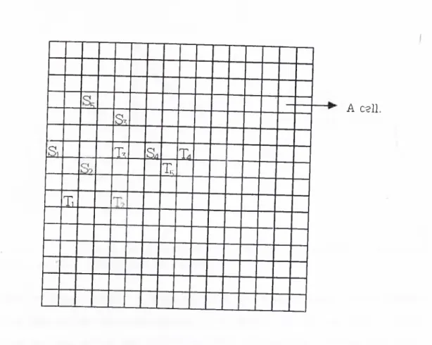
In global routing phase of the layout problem, the routing area can be rep­ resented as a 2-dimensional grid as shown in Fig. 1.1, when one metal layer is used for wiring. The grid (also called global grid) is divided into squares called cells. There are specially designated cells called pins, such as cells Si, Ti, S2, T2 in Fig. 1.1. A net is defined to be the set of pins to be interconnected. For example, the net A^i is denoted by two pins Si and T’l. In Fig. 1.1, all nets have two pins, hence they are called two-pin nets. However, in practice some of the nets may have more than two pins, such nets are called multipin nets. The overall aim in global routing is to realize all the net interconnections using the shortest paths. Here, a path is defined to be the interconnecting wire between the pins of a net. The paths are realized by passing wires through the channels in the cells. The vertical and horizontal lines between neighbor cells rep?'esent the channels. Wires can go from one cell to another adjacent cell by either crossing a vertical or a horizontal channel. Hence, moves from

CHAPTER 1. INTRODUCTION S-I C 'i S· Ti s X X A cell.

Figure 1.1. Grid representation of the wiring surface in gate array layout. a cell are restricted to four directions (south,north,west,east). However, due to the technological constraints, the channels are assigned with a channel ca­ pacity representing the number of wires that can cross that channel. As the interconnections between the pins (net terminals) are constructed some of the cells are declared to be blocked, that is no more wires can pass through those cells. In this work, for simplicity, each cell is assumed to have a wiring capacity of a single wire. If nets are interconnected (routed) one net at a time basis, the global routing phase reduces to maze routing.

Since there may be thousands of nets to be routed, global routing is a time consuming task. Hence, heuristics are used for global routing and maze routing [3, 4, 5, 6, 10]. However, due to the assumptions and constraints they impose, heuristic algorithms may fail to find a path even if one exists. This can be illustrated by Figs. 1.3 and 1.4. In these figures, the routing of nets are done by using a heuristic which allows routing of nets having at most a single

CHAPTER 1. INTRODUCTION

S.

A bend

T (b)

Figure 1.2. (a) Single bend path (heuristic can find such a path) (b) Two-bend path (heuristic fails to find such a path).

bend as shown in Fig. 1.2. After routing a net, the cell capacities are updated and cells on the path are declared as blocked. The routing of net (5s,Ts), however, can not be done by this heuristic, because heuristic can only find a single bend path (dotted lines in Fig. 1.5), which violates the cell capacities of some cells. The re-routing of this net is required. The re-routing of this net can be achieved by exhaustive search of the wiring area. Lee’s maze routing algorithm and Lee type algorithms for multipin nets are such type of exhaustive search algorithms.

These algorithms are computationally expensive algorithms and consume large amounts of computer time for large grid sizes. Hence, these algorithms are good candidates for parallelization. Also, these algorithms require large memory space to hold the wiring grid. Therefore, the effective paralleliza­ tion of these algorithms require the partitioning of the computations cincl the grid among the processors. Hence, these algorithms can be parallelized on distributed-memory message passing multiprocessors (multicomputers).

A multicomputer is an ensemble of processors interconnected in a certain topology. In a multicomputer, each processor has its own local memory and there is no globally shared memory in the system. Each processor runs indepen­ dently (e.synchronously). The cooperation, synchronization and data exchange

CHAPTER 1. INTRODUCTION

s,

Sr

T,

s.

T4

s?

T,

Ti

T?

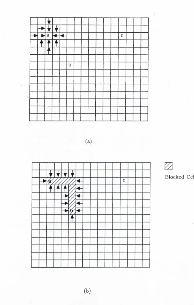
(a) s . i l M T. _S4 T4 m _T, m m ^ 5 Blocked Cell □ Unblocked Cell (b)

Figure 1.3. Routing of nets using heuristic (a) Routing of net {Si^Ti) (b) Routing of net {S2,T2).

CHAPTER 1. INTRODUCTION (a) w i^4 *14

■

Ts (b)

Figure 1.4. Routing of nets using heuristic (a) Routing of net (SsjTs) (b) Routing of net {Si,T^).

CHAPTER 1. INTRODUCTION

Figure 1.5. Heuristic fails to find the path for (.S'5,Ts), because the path (dotted lines) violates cell capacities.

between processors are achieved by explicit message-passing between proces­ sors. Therefore, the interconnection topology plays an important role on the performance of such computers.

Among the many interconnection topologies such as ring, mesh etc., hyper­ cube interconnection topology is the most popular topologjc The popularity of hypercube topology comes from the fact that many other topologies (such as ring, mesh, tree) can be embedded onto hvpercube [11]. In addition, there are commercially available hypercube connected multicomputers such as FPS T-series NCUBE iPSC/1 iPSC/2 A

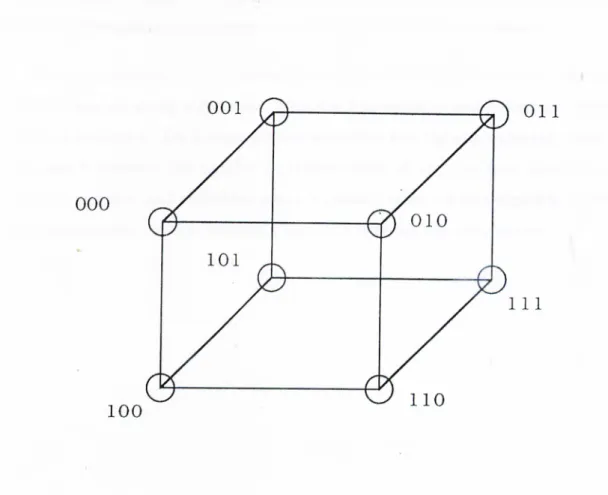
In such an architecture, for a d dimensional h3'percube, there are 2*^ pro­ cessors (nodes). Each node is connected directly to d other nodes. Figure 1.6 represents a 3-dimensional hypercube structure. The binary encoding of a processor differs in only one bit from the neighbor’s encoding. The processors

*FPS T-series is a registered trade mark of FPS Inc. ^NCUBE is a registered trade mark of NCUBE Inc. ^iPSC/1 is a registered trade mark of Intel Inc. ^iPSC/2 is a registered trade mark of Intel Inc.

, CHAPTER 1. INTRODUCTION

Figure 1.6. 8 node hypercube structure

can directly communicate to d neighbors only. The communication between processors that are not connected directly is done through other processors by either software or hardware. Maximum distance between two ¡processors in a hypercube is cl.

Achieving speed-up through parallelism in such architectures is not straight­ forward. The algorithm must be designed so that data and computations are distributed evenly among processors to achieve the maximum load balance. In a parallel machine with high communication latency, the algorithms must be designed so that the large amounts of computations are done between commu­ nication steps. Another factor effecting the parallel algorithms is the ability of parallel systems to overlap the computation with communication. A good par­ allel algorithm should exploit these factors and the topology of the architecture to achieve maximum speed-up.

CHAPTER 1. INTRODUCTION

and Lee type multipin net algorithms on a commercially available multicom­ puter implementing the hypercube connection topolog}' is addressed.

The organization of this thesis is as follows, Chapter 2 presents the se­ quential maze routing algorithms. Chapter 3 presents several different parallel implementations of Lee’s maze routing algorithm and the experimental results. Chapter 4 presents the parallel implementation of two Lee type algorithms, Akers’ algorithm and algorithm using Krusked’s spanning-tree algorithm, and the experimental results. Finally, Chapter 5 presents the conclusions.

2. SEQUENTIAL MAZE R O U T IN G

ALGORITHM S

This chapter presents sequential maze routing algorithms used in exhaustive search of the wiring area. First section describes a well known algorithm, called Lee’s maze routing algorithm [7], for routing two-pin nets. Some nets, however, as is stated in Chap. 1 may have more than two pins. Routing of such nets is the direct translation of Steiner Tree proble7n[lo, 16] into the context of routing in rectangular grids. There are two algorithms that are the variations of Lee’s maze routing algorithm. These algorithms are presented in section 2.

2.1

L ee’s Maze Routing A lgorithm

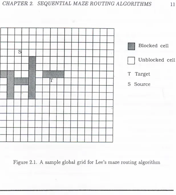
Lee’s maze routing algorithm is a well known algorithm for routing two-pin nets. In the two-pin net problem, the routing area is represented as a two- dimensional grid as shown in Fig. 2.1. Each cell has a status which may be blocked or unblocked initially. This status information is kept in a two- dimensional array called status array. There are two special cells, called source (S) and target (T) (see Fig. 2.1). The aim is to find the shortest path between source and target cells.

Lee’s maze routing algorithm consists of three phases, namely, front wave expansion, path recovery, and sweeping [8]. Front wave expansion phase is a breadth-first search strategy starting from the source cell. The description of the algorithm for the front wave expansion phase is given in Fig. 2.2.

The labeling operation (at Step 2) of a free and unlabeled adjacent cell

CHAPTER 2. SEQUENTIAL MAZE ROUTING ALGORITHMS 11

Blocked cell [ [ Unblocked cell T Target

S Source

Figure 2.1. A sample global grid for Lee’s maze routing algorithm

A queue, called expansion queue, initially contains only the source cell. A queue, called sweep queue, is initially empty. A two dimensional NxN Status array holds the status for the cells of an NxN grid. All the free cells are initially unlabeled.

1. Remove a cell c from the expansion queue.

2. Examine the four adjacent cells of the cell c using the current infor­ mation in the Status array. Discard the blocked and already labeled adjacent cells. Update the status of the unlabtled free adjacent cells as labeled in the Status array and add those cells to the expansion queue. If all adjacent cells of the cell c are either blocked or already labeled, then add the cell c into the sweep queue.

3. Go to step 1 until either target cell is labeled or expansion queue becomes empty.

CHAPTER 2. SEQ UENTIAL MAZE RO UTING ALGORITHMS 12

1. Follow the labels starting from the target cell until the source cell is reached. Label the visited cells as blocked.

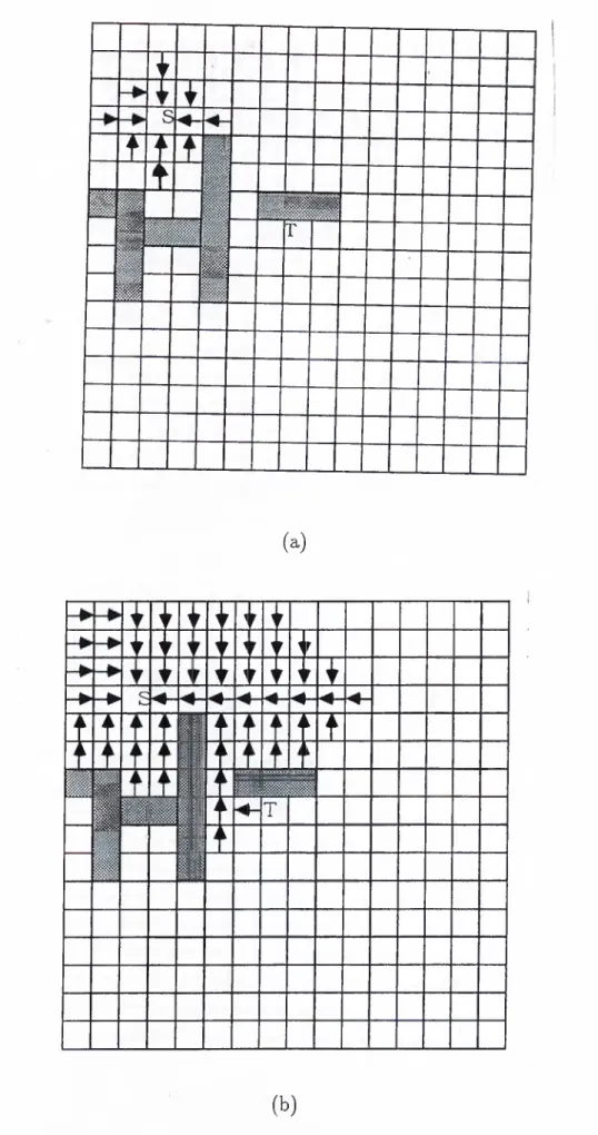
Figure 2.3. Path recovery phase of the Lee’s maze routing algorithm is performed such that, the label points to the cell c being expanded. The algorithm terminates successfully when the tcirget cell t is labeled during Step 2 of the algorithm. The Lee’s maze routing algorithm is guaranteed to find the shortest wire path between the source and the target. The algorithm may also term inate when a remove operation from tin empty queue is attem pted. Such a termination condition indicates the non-existence of a wire-path from the source to the target. Fig. 2.5(a) illustrates the first two cycles of the front wave expansion phase of the Lee’s algorithm for the example grid shown in Fig. 2.1. Labeling process at Step 2 of the algorithm is illustrated by the following four labels, I, ·<—, f, and —»· in the figure. The front wave expansion phase is followed by the path recovery sjadi sweeping phases. Fig. 2.5(b) illustrates the successful term ination of the front wave expansion phase.

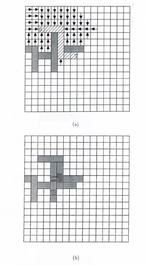
In the path recovery phase, the labels are followed starting from the target cell to construct the path between source and target (see Fig. 2.6(a)). The algorithm is given in Fig. 2.3.

After the path recovery phase is completed, the labeled cells in the front wave expansion phase have to be unlabeled so that next net can be routed. This unlabeling operation is carried out in sweeping phase. The sweeping phase is given in Fig. 2.4.

At the end of front wave expansion phase the expansion queue contains the cells e.xpanded in the last expansion cycle of the front wave expansion phase. These terminal cells are already labeled and connected to their parents. Thus, the cells labeled in the expansion paths starting from the source cell and term inating at these terminal cells can be unlabeled by following their labels (step 2 of the sweep algorithm). However, during the front wave expansion phase, some of the expansion paths initiated from the source cell are blocked

CHAPTER 2. SEQ UENTIAL MAZE RO UTING ALGORITHMS 13

1. Remove a cell c from sweep queue or expansion queue

2. Follow the labels starting from c until a blocked or imlabeled cell is reached. Unlabel the visited cells in the status arra}''.

3. Repeat steps 1 and 2 until both sweep queue and expansion queues are empty.

Figui’e 2.4. Sweeping phase of the Lee’s maze routing algorithm

either due to blocked cells or due to the ¿dread}' labeled cells. The terminal cells of these blocked expansion paths ¿ire ¿idded into the sweep queue at step 2 of the front wave expansion algorithm (see Fig. 2.7). Hence, the cells labeled in these blocked expansion paths should also be unlabeled during the sweeping phase. Fig. 2.6(b) illustrates the final configuration after the path recovery &nd sxoeeping phases.

2.2

Lee T ype A lgorithm s For Routing of M ultipin N ets

The routing of multipin nets is the direct translation of Minimum· Steiner tree problem [15] into the context of routing. The definition of the Mininum Steiner tree problem (or Steiner tree problem) for general gi'ciphs [1] is as follows :

Instance : A connected undirected graph G — (F^, with edge cost function

X : E and a subset R C F of required vertices.

configurations : All edge-weighted trees.

Solutions : All Steiner ¿reesfor R in G\ that is, all subtrees of G that connect aU vertices in R and aU of whose leaves are vertices in R.

minimize : A(T) =

The Steiner tree problem is an NP-hard problem. The existing approxi­ mate algorithms try to find an suboptimril solution in reasonable time. These

represents the vertices of the graph G represents the edges of graph G

CHAPTER 2. SEQ UENTIAL MAZE RO UTING ALGORITHMS ₁₄ n 1 f i 1 t ■ 1 # w m m ■ T • -(a) T T i F T ' P T 1 t _{t ’} j ir ▼ 1 i i ’\ 1 u 1 y n f f i h T (b)

Figure 2.5. Front wave expansion phase of the Lee’s algorithm (a) Initial cycles of front wave expansion phase (b) Successful termination of front wave expansion

CHAPTER 2. SEQ UENTIAL MAZE RO UTING ALGORITHMS 15 (a)

1

w

mm

III

(b)

Figure 2.6. Path recovery and sweep phases of Lee’s algorithm after the front wave expansion phase (a) Path Recovery phase (b) Final configuration after- sweep phase

CHAPTER 2. SEQUENTIAL MAZE ROUTING ALGORITHMS ₁₆ T P I * -► ^1

s

◄-

_{p X i}

f f f f t

iM ii

mMmi

ipiiil

Figure 2.7. The use of the sweep queue, cells marked as 1,2,3 are added into the sweep queue at expansion cycles 3,3, and 2, respectively.

CHAPTER 2. SEQUENTIAL MAZE ROUTING ALGORITHMS 17

approximate algorithms try to find a good Steiner tree by combining minimum- spanning-tree and shortest path calculations. The cost of the Steiner tree Tsub, on grid graphs, found by these algorithms is bounded by

Cosi{Tsub) < -Cost{Topt) (2.1)

as shown in [16], where CosiiTsub) is the cost of the suboptimal tree and Cost{Topi) is the cost of optimal Steiner tree. In this work, parallelizaiion of two algorithms that use Prim ’s and Kruskal’s algorithms [1] for rninimum- spanning-tree calculations and Lee’s maze routing algorithm for the shortest path calculations is addressed. Following two sections present the sequential versions of these algorithms.

2.2.1

U sing P rim ’s Algorithm

Using P rim ’s algorithm [1], Akers[l, 17] has developed an algorithm to route multipin nets. The algorithm uses Lee’s routing algorithm for the connection of pins. P rim ’s algorithm is used for solving the minimum spaniiing tree problem. Akers’ algorithm is a modification of this algorithm into the Steiner tree prob­ lem. The pins in the multipin net are called the terminal cells. The algorithm is given in Fig. 2.8.

At step 2 of the algorithm, the set of sources consists of all the visited cells during the previously and currently constructed respective shortest iDaths. The propagation of the new front waves starts from all of these cells taking them as new sources. Fig. 2.9 and 2.10 illustrates the steps of the Akers’ algorithm for connection of a multipin net.

CHAP TER 2. SEQ UENTIAL MAZE RO UTING ALGORITHMS 18

1. Choose an arbitrary pin of the net and perform Lee’s front wave expansion phase to propagate a unidirectional search wave starting from this pin cell until it hits another terminal cell.

2. Perform path recovery to construct the respective shortest path. Add all the cells visited during the path recoveiy phase into the set of sources.

3. Perform the sweeping phase to unlabel all labeled cells during step 2 for the next search wave.

4. Propagate unidirectional multi-search waves stcirting from the set of multi-sources in the expansion queue until an unlabeled terminal cell is reached.

5. Goto step 2 until all terminal cells of the net are labeled.

Figure 2.8. Sequential version of the algorithm for routing multipin nets usin| Prim ’s algorithm

2.2.2

Using KruskaPs A lgorithm

If we base the Steiner tree computations onto Kruskal’s algorithm [1] a faster algorithm [1] can be derived for the connection of multipin nets. This algo­ rithm basically propagates search waves starting from all required pins (term i­ nal cells). The algorithm using Kruskal’s spanning-tree algorithm (Kruskal’s Steiner tree algorithm) is given in Fig. 2.1 1. At the beginning all pins form a distinct tree. During the search phase of the algorithm when two search waves starting from different trees collide these two trees are merged and a new tree is formed. There are two procedures to perform the above mentioned task. UNION{ci,Cj) merges two different trees to which c,· and Cj belong.

TR EE ( Ci ) returns the tree that c,· belongs to. Since each cell may belong to different trees, the status information of a cell in status array indicates both the label status (labeled, unlabeled, blocked) and a tree information to be used in procedures T R E E { c i ) and U N I O N { c i , C j ) . Fig. 2.12 shows the routing of a single three pin net using this algorithm.

CHAPTER 2. SEQ UENTIAL MAZE RO UTING ALGORITHMS 19

T

- > _T

₁

a C

T

n

T

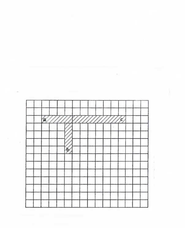
n b (a) 7 / Blocked Cell (b)

Figure 2.9. Front wave expansion phase of the Akers’ algorithm beginning from the terminal cell ’a ’ (a) initial two cycles (b) Initial cycle after the first path (a to b) is connected.

CHAPTER 2. SEQUENTIAL MAZE ROUTING ALGORITHMS 20

y ////////////A

CHAPTER 2. SEQ UENTIAL MAZE RO UTING ALGORITHMS 21

1. Add all the terminal cells into the expansion queue.

2. Perform Lee’s front wave expansion phase to propagate multi search waves starring from all terminal cells.

(a) choose-a cell c from queue and examine its adjacent cells a fs for expansion.

(b) If c . is a free cell then add Oc to expansion queue, label the cell to point to the parent cell c and update the tree information of Uc in status array so that the cell Uc belongs to the same tree as its parent.

(c) If is labeled and T REE{uc) is not ec|ual to TREE{c) this indicates the collision of two different front waves (search waves), then call U N IO N {c,ac). Save the pair of colliding adjacent cells.

(d) If TREE{ac) = T R E E {c) or Oc is blocked, ignore the cell

a , .

(e) If all four adjacent cells a fs of cell c are blocked or labeled such that they belong to the same tree with the cell c then add the cell c to the sweep queue.

3. Repeat step 2, until all trees are merged.

4. Perform path recovery starting from the collision points of different trees to form the interconnections between required pins.

5. Perform the sweeping phase.

Figure 2.11. Seciuential version of the algorithm for routing multipin nets using Kruskal’s algorithm

CHAPTER 2. SEQ UENTIAL MAZE RO UTING ALGORITHMS ₂₂ n u n n

1

a _{c *4-}<

-T t

_n

_{T t t}

_f

u n

1

-> ->> b ◄--4-f

t

t (a) Blocked Cell (b)

Figure 2.12. Routing of a three pin net using Kruskal’s algorithm (a) Initial cycles of the algorithm (b) After connecting all pins

3. PARALLELIZATION OF LEE’S

ALGORITHM

This chapter presents the principles and ideas used for the parallel imiDlemen- tation of Lee’s algorithm. Lee’s algorithm is a special case of m ultipin net algorithms. The ideas and principles for parallel implementation of Lee’s al­ gorithm will then be adopted for the parallel implementation of m ultipin net algorithms.

As indicated in Chapter 2, the Lee’s Maze Routing algorithm consists of three phases, namely front wave expansion^ path recovery, sweeping phases. Each phase of the algorithm has been parallelized, and the following sections present the proposed parallel algorithms for three phases. Each phase is con­ sidered independently.

The secjuential complexity of the Lee’s maze routing is due to the front wave expansion and sweeping phases. As is discussed in Section 3.2, the par­ allel front expansion scheme proposed in this chapter avoids interprocessor communication during the distributed sweeping phase computations. How­ ever, interprocessor communication can not be avoided during the distributed front wave expansion phase computations. Furthermore, as is discussed in Section 3.1, the processor utilization during the distributed front wave expan­ sion computations is very sensitive to the grid partitioning scheme employed. Hence, the grid partitioning and mapping scheme is chosen by mainly consid­ ering the computational requirements of the front wave expansion phase.

CHAPTER 3. PARALLELIZATION OF LEE’S ALGORITHM 24

3,1

Grid Partitioning and M apping

The effective parallel implementation of the front wave expansion algorithm on a hypercube multicomputer requires the partitioning and mapping of the expan­ sion computations and the data structures associated with the grid (i.e. status array). This partitioning and mapping should be performed in a manner that results in low interprocessor communication overhead and low processor idle time. Even partitioning of the status array onto the node processors is an easy task since a fixed size two dimensional grid is to be partitioned and mapped to the processors of the hypercube. Even partitioning of the exi)ansion computa­ tions, on the other hand, is not easy because expansion computations are not predictable and depends on the data (blocked cells etc.). However, as will be explained later, the partitioning of the status array affects the partitioning of expansion computations, and as a result, affects the processor utilization and interprocessor communication overhead.

In the front wave expansion phase, the atomic operation can be considered as the expansion of a single cell in the current front wave. In this atomic pro­ cess, the north, east, south, and west adjacent cells of the cell being expanded are examined. Hence, the nature of communication required in front wave ex­ pansion phase corresponds to a two dimensional mesh. That is. each processor needs to communicate only to its north, east, south, and west neighbors. Hence, onl}' mesh embedded hypercube structure will be considered and partitioning and mapping of the grid is done considering only a mesh embedded hypercube structure. It is well known that, a processor mesh can be embed­ ded into a (¿-dimensional hypercube [1 1]. Fig. 3.1(a), (b), and (c) represent the mesh’embedding into hypercubes of dimensions 2, 3, and 4, respectively.

The even partitioning and mapping of the global status array is trivial since a two dimensional N x N mesh grid is to be partitioned and mapped onto a two dimensional mesh embedded hypercube. This mapping can be achieved by applying tiled decomposition in partitioning the grid. Assume that N is a power of two (i.e. N = 2") and n > [<¿/2]. In the tiled decomposition, the grid is covered with rectangles of size 2”“ l‘^/^Jx2"'“ f‘^/^l starting from the top left corner and then proceeding left to right and top to bottom. Each rectangle cover

CHAPTER 3. PARALLELIZATION OF LEE’S ALGORITHM 25 (a)

—

( ] ^

—

- / i v

- / T o (b ) 0100) 1000

)

0111 0010 1110

1010

(c)

Figure 3.1. Mesh embedding (a) h}'’percube of dimension 2 (b) hypercube of dimension 3 (c) hypercube of dimension 4

CHAPTER 3. PARALLELIZATION OF LEE’S ALGORITHM 26 0

0

0 0 D“ 0 0 0 0 3 O' Ü" 5·

0 0

Ü“ 0 3 O' 3· ÜT 0

0

0 3 3 3“ 4 7 6^ 4 7

6

6 6 3" w b 5 5 7 7 7

6

6

W~E

6

Ü" 4 4 4 7 7 7 5 5 7 7

6

6

6

6

4 4 4 4 5 5 7 4 4 4 4 6 6 6 6

Figure 3.2. Tiled decomposition of a 16x16 grid onto 2x4 mesh embedded

3-dimensional hypercube

defines a partition of the grid. These partitions are then mapped to processors in such a way that, partitions that are adjacent in the grid are mapped to adjacent processors of the processor mesh embedded in the h}^percube. In this mapping, each processor will be responsible for holding and updating the status information (local status array) for the cells belonging to its local grid partition. Each processor will be responsible for the expansion computations for the cells in its local grid partition. Figure 3.2 illustrates the tiled partitioning scheme for a 16x16 grid for a 2x4 mesh embedded 3-diraensioncil hypercube.

In the given mapping scheme, a grid cell is defined to be a boundary cell if and only if at least one of its neighbor cells (i.e. north,east,south, west) is in a different partition. It is obvious that only boundary cells have a potential to cause interprocessor communication. The volume of possible interprocessor communication can be reduced by decreasing the number of boundary cells. It is well known that the number of boundary cells in a rectangular partition

CHAPTER 3. PARALLELIZATION OF LEE’S ALGORITHM 27

with fixed number of cells can be minimized by choosing a square partition. The proposed mapping scheme achieves square partitions for even dimensional hypercubes (i.e. even d). For odd dimensional hypercubes the partitions are rectangles with long sides only twice the short sides. .Such rectangle partitions minimize the number of boundary cells while maintaining the perfect balanced partitioning of the status array.

The tiled decomposition scheme ensures the mesh communication topology and even distribution of the data structures (status array] among the proces­ sors of the hypercube. This mapping scheme also minimizes the volume of interprocessor communication during the front wave expansion phase. How­ ever, in spite of these nice properties, it does not ensure the even distribution of the front wave expansion computations. Assume that, in Fig. 3.2, the .source cell and the target cell are located at the top left and bottom right corner of the global grid, respectively. Also, assume th at there are no blocked cells in the grid. During several initial cycles, only processor Pq will perform front wave

expansion computations while remaining processors stay idle. Similarl}'·, during several final cycles, only Pq will be busy with front wave expansion computa­ tions while the remaining processors stay idle. Hence, the tiled decomposition scheme yields very low processor utilization.

Processor utilization can be maximized by applying scafrereddecomposition scheme. Scattered decomposition scheme is achieved by imposing a periodic processor mesh template over the grid cells starting from the top left corner and proceeding left to right and top to bottom . Figure 3.3 illustrates the scat­ tered decomposition of a 16x16 grid for a 2x4 mesh embedded 3-dimensional h3'^percube. In this scheme, adjacent grid cells in the grid are assigned to adjacent ¡processors of the mesh embedded hypercube, thus ensuring the mesh communication topology. This scheme also ensures the even distribution of the status array among the processors of the hypercube. Howe^■er, in the scattered decomposition, all local cells assigned to individual processors are boundary cells. In fact, for d > 2, all four neighbors of an individual local cell beloirg to adjacent processors. Hence, the expansion of any local cell in all four directions require interprocessor communications. Thus, scattered decomposition scheme causes large volume of interprocessor communication.

CHAPTER 3. PARALLELIZATION OF LEE’S ALGORITHM ₂₈ IT1

3^

1

3^ 3^ f r

1

3“ 3^ 3^

1

3“ 3“

4 5 7 6 4 5 7 6 4 5 7 6 4 5 7 6

0

1 5

3 0

1

3 3 0

1

3 3 0

1

3 3

4 5 7 6 4 5 7 6 4 5 7 6 4 5 7 6

0

1 5

3 0

1

3 3 0

1

3 3 0

1

3 3

4 5 7 6 4 5 7 6 4 5 7 6 4 5 7 6

0

1 5 3

0

1

3 3 0

1

3 3 0

1

3 3

4 5 7 6 4 5 7 6 4 5 7 6 4 5 7 6

0

1

3 3

0 1

3 3

0 . 1

3

2

0

1

3 3

4 5 7 6 4 5 7 6 4 5 7 6 4 5 7 6 0 1

3 3

0 1

3 3

0 1

3 3

0 1

3 3

4 5 7 6 4 5 7 6 4 5 7 6 4 5 7 6 0 1

3

3 0 1

3 3

0 1

3 3

0 1

3

3 4 5 7 6 4 5 7 6 4 5 7 6 4 5 7 6 0 1

3 3

0 1

3 3

0 1

3 3

0 1

3 3

4 5 7 6 4 5 7 6 4 5 7 6 4 5 7 6

CHAPTER 3. PARALLELIZATION OF LEER ALGORITHM 29

The analysis of these two decomposition schemes shows th at there is a trade-off between processor utilization and volume of interprocessor communi­ cation. This trade-off is resolved by combining tiled and scattered decomposi­ tion schemes as is also proposed in [8]. In this scheme, NxN grid is transformed into a coarse grid by applying tiled decomposition assuming much larger P1XP2

mesh processor array, where Pi and P2 are powers of two. Pi = P2 for even d, P2 = 2Pi for odd d, and P1XP2 ^ 2^^ but Pi and P2 < N. Hence, effectively the NxN grid is covered with hxw rectangle (or square) subblocks where h = w = ^ and h,w values are power of two where h C N. Then, scattered decomposition is applied to the generated coarse grid. That is, a periodic processor mesh template (of size 2NPJx2N/N) is imposed over the hxw grid subblocks starting from the top left corner and proceeding left to right and top to bottom. Figure 3.4 shows the maiaping of 2x2 and 4x2 grid subblocks over a 16x16 routing grid to the processors of a 2x4 processor mesh embedded in a 3- dimensional hypercube. In this scheme, h = w for even li3'percube dimensions and h = 2w for odd hypercube dimensions. The width w of the rectangles con­ stitutes the characteristic of the decomposition. This mapping scheme reduces to scattered mapping scheme when h — w — I [Pi = P2 = N ) and it reduces to tiled decomposition scheme when h — and w — (A = 2N/^-l and P2 = The processor idle time will decrease with decreasing w. However, the volume of interprocessor communication will decrease with increasing w. Hence, the trade-off between processor utilization and volume of interprocessor communication can be resolved by selecting an appropriate value for w.

3.2

Parallel Front Wave Expansion

3.2.1

Expansion Starting From Source Only

The expansion starting from source only (Sonly j scheme initiates a breadth first search starting from the source cell as in the original Lee’s algorithm[7]. The status array is partitioned and mapped onto the node processors according to the mapping scheme presented in section 3.1. Hence, each processor stores and maintains a local status array to keep d3mamic and static status information

CHAPTER 3. PARALLELIZATION OF LEE’S ALGORITHM ₃₀ w

i

0 (T 1 1 3 3 2 '2“ 0 i r 1 1 3 3~ 2 ■2~ u U _{1 1 3 3 2 2 0 0 1 1 3 3 2 2} 4 4 5

6

7 7 _{6 6 4} 4 5 3 7 7 6 3” 4 4 5 5 7 7 6 6 4 4 3 3 7 7 6 0 U _{1 1 3 5 2 2 0 0 1 1 3 3“ 2 2“} 0 0 _{1 1 3 3 2 2 0 0 1 1 3 3 2 2} 4 4 5 5 7 7 6 6 4 4 ,5 3“ 7 7 6 3“ 4 4 5 5 7 7 6 6 4 4 3 3~ 7 7 6 6 0 0 _{1 1 3 5 2 2 0 0 1 1 3 2 2“} 0. b 1 1 3 8 2 2 0 0 1 1 3 b~ 2 2 4 4 5

6

7 7' 6 6 4 4 3 3 7 7 6 5“ 4 4 5

6

7 7 6 6 4 4 5 3~ 7 7 6 6 0 0 1

1

3 3 2 2 0 0“ 1 1 ' 3 3~ 2 2“ 0 0 1 1 3 3 2 2 0 0 1 3 3 2 2 4 4 5 'b 7 7 6 s 4 4 3 3 7 7 6 3 4 4 5 13 7 ■7 8 3 4 4 3 3 7 '7 D— w (a)

f r

1 1

3

3^ 2 2^ i r i r 1 1

3

3^ 2 2^

0

0

1 1

3 3

2 2 0 0 1 1

3 3

2 2

0 0 1 1 5 3 2 2 0 0 1 1 3 3 2 2

0 0 1 1

3 3

2 2 0 0 1 1

3 3

2 2

4 4 3

3

7 7

_{6 6}

4 4 3

3

7 7

_{6 6}

4 4

5 3

7 7

6 6

4 4

3 3

7 7

6 6

4 4·

3

3

7 7

6 6 4

4

3 3

7 7

3 8

4 4

5 3

7 7

6 6

4 4

3

3

7 7

6 6

0 0

1

1

3

3 2 2 0 0 1 1 3 3 2 2

0 0

1

1

3 3

2 2 0 0 1

1 3 3

2 2

0 0

1

1 3 3 2 2

u u

1 1

3 3

2

2

0

b

1

1

3

3

2 2

u

0 1 1

3 3

2

2

4 4

_{5 3}

1 7

6 6

4 4

₃

b 7 7

₈

fc)

4 4

5 3

7 7

6 6

4 4

5 5

7 7

3

4 4

3

3

7 7

6 6

4 4 b b 7 7

3

3

4 4

5 3

7 7 6 6 4 4 5

5

7 7 6 3 h

(b)

Figure 3.4. Decomposition of 16x16 grid into subblocks of (a) h (b) h = 2w = 4

CHAPTER 3. PARALLELIZATION OF LEE’S ALGORITHM 31 N o rth S en d W e s t S e n d W e s t R e c V N orth R ecv

Ix>cal E xp ansion Q ueue Local S w eep Q ueue

S o u th S en d

Local Grid

S outhR ecv

Figure 3.5. Local data structures for a node processor.

for its local cells. Each processor maintains a local expansion queue to process the front wave expansion for its local cells. Each processor also maintains a local sweep queue to store the blocked expansion paths for the sweeping phase. As is indicated in Section 3.1, the expansion of each local boundary cell require communication with at least one neighbor processor. Hence, in order to accompli.sh that communication, each processor also maintains four different send queues [north, east, south, and loest send queues) for storing and transmitting cell coordinate information to its four neighbor processors in the mesh. Similarly, each processor maintains four receive queues to store information sent by its four neighbor processors. Fig. 3.5 illustrates the view of the local data structures for a node processor. The parallel algorithm is given in Fig. 3.6

The local x and y coordinates of the local cells in the current wave are stored in the local circular queues. One byte word Status[x,y) is allocated in

CHAPTER 3. PARALLELIZATION OF LEE’S ALGORITHM 32

Imtiallз^, all the local queues are empty. The host processor broadcast the coordinates of the source cell and target cell to all processors. The processor which owns the source cell location adds the local coordinates of the source cell to its local queue. Then each processor executes the following algorithm.

1. Each processor examines the cells in its local expansion queue for expansion in four directions. The local adjacent cells of the cells being expanded are examined for adding them to the local expansion queue for later expansion. The adjacent cells which are detected to belong to grid partitions assigned to neighbor processors are added to the corresponding send queues for later communication.

2. Each processor transmits the information in its f< 'ir send ciueues to their destination processors.

3. Each processor examines the cells in its four receive queues for adding them to its local queue for later expansion.

4. Each processor repeats steps 1, 2, and 3 until host signals the ter­ mination of the front wave expansion phase.

Figure 3.6. Node program for the Sonly scheme

the two dimensional local status array for the status information of each local cell. The encoding of the status of a cell is shown in the Figure 3.7. The least significant three bits (bits 0,1,2) of S ta tu s{x,y) hold the current routing status of the local cell located at the local x and y coordinates. Six different routing status information are; blocked, unlabeled, and labeled from north, east, south and west. The status information is obtained by examining Tie value of these three bits. The values and the meanings are

000 : Unlabeled 001 : Blocked

010 : Labeled from North (Connected to North) 011 : Labeled from South

100 : Labeled from West 101 : Labeled from East.

CHAPTER 3. PARALLELIZATION OF LEE’S ALGORITHM 33

7 6 0

T arget Mark

f Sp aü al O rientation f e n co d in g f ▼ of the cell.

T

routing s ta tu s T

of cell

Figure 3.7. Encoding the status information

As is discussed earlier, the expansion of a boundary cell necessitates inter­ processor communication. Hence, each processor should store spatial orienta­ tion information in its status array for its local cells. Four bits (bits 3,4,5,6) in the one byte word are reserved for spatial orientation information in the local grid of the processor. The assertion of a particular bit indicates that the cell is in the local partition boundary in the corresponding expansion direction. That is, the adjacent cell in that expansion direction is not a local cell, and it is assigned to the neighbor processor in th at expansion direction. Hence, that adjacent cell should be added into the particular send queue in that expansion direction. Note that, a cell may be a boundary cell in more than one expansion directions. For example , if bit 65 and bit Iq is asserted then the cell is at the north-west boundary. Also note that, bits 66^5^4^3 = 0000 indicates that the cell is a local interior cell whose four adjacent cells belong to the local grid par­ tition. This bitwise horizontal encoding scheme for spatial orientation is chosen in order to decrease the complexity of the local expansion computations.

Whenever, the processor which owns the target cell labels the target cell, (either at Step 1 or Step 3), it signals the host about the successful termination. The host processor, upon receiving such a message, broadcasts a message to all processors to terminate the front wave expansion phase and enter into the path recovery phase. Then, the processor which owns the target cell initiates a path recovery beginning from the target cell.

CHAPTER 3. PARALLELIZATION OF LEE’S ALGORITHM 34

If a cell is found to belong to the partition assigned to a neighbor processor, the x,y coordinates of the cell are put into the corresponding send queue and sent to the neighbor processor. Plowever, due to the partitioning of the global grid onto processors, each cell in a processor’s local grid has local coordinates. Hence, when the non-local adjacent cell Oc of a boundary cell c is transferred to a neighbor processor, the x,y coordinates of the cell have to be converted to the local coordinates in the receiving processor. This conversion operation is an overhead associated with the pcirallelization. The expcinsion computa­ tion associated with an individual cell has fine granularity. Hence, an efficient scheme should be devised for this conversion in order to keep this overhead low. This conversion can be performed using two schemes. In the first scheiiie, the local coordinates of the cell is converted to global coordinates and then to the local coordinates of the receiving processor. Such an operation is computation­ ally exjDensive operation. In the second scheme, the local-to-local conversion is achieved directly. This efficient scheme is briefly discussed in the following paragraph.

Note that, the left-top corner of the global grid (and local grids) is chosen as the origin of the x-y coordinate system. Hence, x-coordinate increases in east direction and y-coordinate increases in the south direction. In the proposed mapping, grid cells in a particular row (column) of the global grid are par­ titioned into successive contiguous blocks of size w (h). Then, successive cell blocks in a row (column) of the global grid are mapped to the successive proces­ sors in a periodical!}'' repeating row (column) of the processor mesh template. Hence, local x-coordinates (y-coordinates) of a boundary cell between two suc­ cessive processors in an individual mesh template differ by w (h). However, if a cell is a boundary cell between two boundary processors in a row (column) of the repeating processor mesh template, then its local coordinates are equal in these two adjacent processors. Note that, local y-coordinates (x-coordinates) of all cells in the same row (column) of the global grid are equal in all processors. Fig. 3.8 illustrates the local indexing of the local status arrays for the mapping of 16x16 grid to a 4x4 mesh embedded 4-dimensional hypercube. As is seen in this figure, w should be added/subtracted for the local-to-local conversions during the east-west communications between the following pairs of adjacent

CHAPTER 3. PARALLELIZATION OF LEE’S ALGORITHM 35

processors (12-13, 13-15, 15-14), since 12-13-15-14 constitute a row of the pro­ cessor mesh template. There is no need for conversion during the east-west communications between the pair of adjacent processors (14-12), since this pair of adjacent processors is the boundary processors of the repeating processor mesh template. Similarly, h should be added/subtracted for the local-to-local conversion during the north-south communications between the following pairs of adjacent processors (1-5, 5-13, 13-9), since 1-5-13-9 constitute a column of the processor mesh template. There is no need for conversion during the north- south communications between the pair of processors (9-1), since this pair of adjacent processors is the boundary processors of the repeating processor mesh template.

In this scheme, each processor statically determines the number to be added for the local-to-local conversion for each boundary expansion direction by ex­ amining its particular location in the processor mesh template. Hence, the overhead associated for the local-to-local conversion required during the ex­ pansion of a boundary cell in the boundary direction is only a single addition operation.

In spite of the given partitioning scheme, the above parallel algorithm may result in low processor utilization for large h and w values. Some processors may still stay idle particularly during the initial and final front wave expansion cycles. This is due to the expansion of a single front wave beginning from the source cell. Note that, finding a routing path from source to target is equivalent to finding a path from target to source. Hence, two front waves^ one beginning from the source {source front wave) and the other one beginning from the target [target front ivave), can be expanded concurrentljc If the source and the target cells are assigned to different processors, this scheme has a potential to increase the processor utilization.

3.2.2

Expansion Starting From Source and Target

This scheme initiates breadth first search starting from the target cell as well as starting from the source cell[14]. Figure 3.9(a) illustrates the initial two cycles of this scheme for the example grid shown in Figure 2.1. The P'igure 3.9(b)

CHAPTER 3. PARALLELIZATION OF LEE’S ALGORITHM ₃₆ local X coordinates --- --- ► 0 1 0 1 0 1 0 1 2 3 2 3 2 3 2 3 local y Coord. 0 1 0 1 0 1 0 1 2 3 2 3 2 3 2 3

€

·!··

....

3

0

....I···

...3 .... ....

2

■

-5··

.... J . . .

6

4

J

5····

6

2

1 3

₁₅

..14)..

₂

₁₃

₁₅

₁

4 )

...g

_a

_{1 1}

_iO

₈

₉

_{•ii····}

_1G

()

3

...2....

0

1

2

. ..

...21

R..

7... . ...A.... . . .AXJ

....7.... G

li

2

13

1

14

12

13

15

14

...a

9

:

1 1

10

8

9

1

10