Optical implementation of the two-dimensional fractional Fourier transform with different orders in the two dimensions

(1)

ELSEVIER

Optics Communications 120 (1995) 134-138 15 October 1995

OPTICS

COMMUNICATIONS

Optical implementation of the two-dimensional fractional Fourier

transform with different orders in the two dimensions

Aysegul Sahin a, Haldun M. Ozaktas a, David Mendlovic b

a Department of Electrical Engineering, Bilkent University, TR-06533 Bilkent, Ankara, Turkey

b Faculty of Engineering, Tel-Aviv University, 69978 Tel-Aviv, Israel

Received 26 April 1995

Abstract

Previous optical implementations of the two-dimensional fractional Fourier transform have assumed identical transform orders in both dimensions. We let the orders in the two orthogonal dimensions to be different and present general design formulae for optically implementing such transforms. This design formulae allows us to specify the two orders and the input, output scale parameters simultaneously.

1. Introduction

The fractional Fourier transform of order a is defined in a manner such that the common Fourier transform is a special case with order a = 1 [ 11. The one-dimensional fractional Fourier transform of order a can be defined for 0 < Ial < 2 as

3=[{f(u)}l(u>

= 7 &Cu, u’>fCu’)

du’

,

-m

(1)

B,Cu uII = exp[-j(&/4

- 9/2>1

Jrn

exp[jlr( u* cot q5 -

2~’

csc C$ + u’* cot 4) 1 ,

(2)

where q!~ = a7r/2 and C$ = sgn( sin4). The kernel is defined separetely for a = 0 and a = 2 as Bo( u, u’) = S( u - u’) and B~(u, u’) = 6( u + u’). The definition can easily be extended outside the interval [ -2,2] by noting that 34j+a (u) =

3a(u).

Some essential properties of the fractional Fourier transform are: (i) It is linear. (ii) The first order transform (a = 1) corresponds to the common Fourier transform. (iii) It is additive in index, 3*l3”4 = 3a1+az4.

The fractional Fourier transforming property of quadratic graded index media was discussed in Refs. [ l- 5,171. Bulk optical systems that realize fractional Fourier transforms were presented in Refs. [ 7,8,10]. Several applications of fractional Fourier transforms were presented in Refs. [ 1,6,7,13]. It was also shown that the

(2)

A. Sahin et al. /Optics Communications 120 (1995) 134-138 135 fractional Fourier transform can be used to describe optical beam propagation and as a tool for analyzing optical systems composed of thin lenses and sections of free space [9,14-161.

The definition of the 2-D fractional Fourier transform is generally made by using the same order in both directions. In this paper we define the 2-D fractional Fourier transform with different orders in the two dimensions. The kernel for this transform is nothing but the product of two 1-D kernels. The 2-D fractional Fourier transform with order a, along the x axis and uy in the y axis is defined as

~a~‘=v’{f(~,u)}](u,v) = ~B,,=.(u,u;u’,o’)f(u’,~‘)d.‘du’, (3)

where

B

o,,aJw~‘,~‘) = &xb,u’~B~y(u,u’h

We interpret U, u’, u, u’ as dimensionless variables.

(4)

Such anamorphic fractional Fourier transforms are necessary in order to generalize previously suggested optical signal processing and filtering schemes to two dimensions [ l-5,13]. Since the characteristics of the signals in the two dimensions may vary, the optimal filtering may require fractional transforms with different orders in the two dimensions. Schemes for realizing anamorphic optical fractional Fourier transforms of variable orders are also essential for tomographic complex wave-field reconstruction techniques [ 11,121.

In this study an optical system for performing the 2-D fractional Fourier transform with different orders is presented. This system allows us to realize 2-D fractional Fourier transform with the desired orders and input, output scale parameters.

2. Optical system for performing 2-D fractional Fourier transform

The suggested system which realizes two-dimensional fractional Fourier transform can be seen in Fig. 1. Each anamorphic lens appearing in the figure may be composed of two orthogonally situated cylindrical thin lenses with different focal lengths.

In the following analysis we determine the focal lengths and separations of the lenses so that ~,,“r( x, y) is the 2-D fractional Fourier transform of pi,(x, y). Let pt (x, y) denote the light distribution after a propagation of distance dl in free space. pin (x, y) and pr (x, y) are related to each other by a simple convolution relation:

Pin PI Pz P3 PO”,

(3)

136 A. Sahin et al. /Optics Communications 120 (1995) 134-138 *cm

PI (x, Y> = exp(-_iaP) h exKiW ss

Pin(x’,y’)exp(jr[(x-X’)‘+(y-y’)*l/A}dx’dy’. (5)

-cu --m

The first lens in the figure has focal length fX in the x direction and fY in the y direction. The light distribution immediate to the right of the first lens is:

Propagation in the second section of free space results in another convolution. The light distribution just before the second lens is:

P~(x,Y) =ev(-j~/2)-&exp(_W)

JJ

pz(x”,y”)exp(jr[(x-n”)*+(y-y”)*]//\}dx”dy”. (7)

-co --oo

The second lens has focal lengths f: and

fi.

This final lens will not affect the light intensity. If we are interested in only the light intensity, there is no need to use these lenses at the output.

After some algebraic manipulations pout(x, y) can be written in terms of pi”(x, y) as follows: moo

Pout(K Y) = IS

Kexp[j?r(x*Al -

2.dA2

+x’*A3

+Y*Bl -

2yy’B2 +Y’*B3)]pin(x’,Y’) dx’dy’, (8) --DC) --oo where K = exp(-j~/2) evLiQ4 + d2)l J fxfr A (d2fx + dlfx - dldZ)(d2fy + dlfy - dld2) ’

A, =

fx -dl 1 A(d2fx - dlfx - dld2) --, Af;

A2 =

1

B1 =

f, -dl

--

A(d2fy - dlfy - dld2) Af; ’ B2 =

fx

_{A3 =}

fx - d2

A(d2fx - dlfx - dld2) ’ A(d2fx - dl fx - dld2) ’

fy - dl

_{B3 =}

fy -dl

Nd2fy - 4fy - dld2) ’ A(d2fy - dlfy - dld2) ’

(9) Remember that x,x', y, y’ etc. have dimensions of length. Thus, in order to put this equation in a form comparable with Eq. (2), we need to introduce the dimensionless variables UI = x/q, 4 = X//ST, 01 = y/s, and u2 = y//s*. Here ~1 and ‘s:! are real valued positive scale parameters with dimensions of length. Also introducing the hatted functions Ijout(~t,ul) = Pout(U1sl,qsl) and &(zQ,u~) = Pin(u2s2,v2s2), Eq. (8) can be written as

0000 &It(~1,Q) =

ss

s$exp[ja(ufsfAt

- ~UIU~SISZA~

+ &~A31

-m --m

x

exp[jr(ufsTBl

-

2~1~2~1~2B2 +v~s~B~)]&(u~,v~)~u~~zJ~. (10) We wish this to represent a fractional Fourier transform relation with the specified orders and scale parameters. By comparing Eq. (3) and Eq. ( lo), we obtain the following necessary and sufficient equations:

s:A, =

cot 4x , s1

s2A2 = csc &

,

$A3 =

cot C/J* ,

(4)

A. Sahin et al. /Optics Communications 120 (1995) 134-138 137

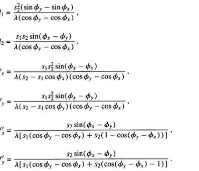
These equations can be solved after some straightforward yet lengthy algebraic manipulations. If dx = q5Y, the equations will simplify and one recovers Lohmann’s results [ lo]. When & # r&, these equations can be solved for the lens focal lengths and separations as functions of the desired orders and scale parameters:

dl = d2 =

fx =

_fY

=

si(sinq$ - sin+x) h(cos& - cos&) ’ (12) sls2 sin(4x - &) A(cos& - cos&) ’ (13) ~1s; sin(& - &)

A(SZ -stcos~,)(cos~y -cos$,) ’ (14)

st$ sin(6 - &)

h(S2-StCOS#~))fCOS~y -cos&) ’ (15)

~2 sin(h - 4y) _HA;\

f: =

Ms1(cos&‘-cos4x) +32(1 -cos(&

-6))l

’

\ Iv)

f; =

~2 Wh - &>

Ns1(cos4, -cos4x) +~2(cos(45 - 4x1 -

1)l *

(17)

Thus by choosing the focal lengths and separations of the lenses as given above, we can optically realize a two-dimensional fractional Fourier transform with orders +x, & and scale parameters st and ~2. Notice that dl and d2, as given by Eq. (12) and Eq. (13), may turn out to be negative. In such cases we would have to deal with virtual objects and/or images. This would require the use of additional lenses. In the event that we wish to avoid this, we must require that dl and d2 be positive. This will then restrict the range of a, and uY, that can be realized. This range can be maximized by allowing the n and y axes to be flipped. For instance, with & = 60 and & = 30, we obtain a negative dl value. This transform is equivalent to the fractional Fourier transform with 4, = 60 and q5,, = 210 followed by a flip of the y axis. (This is because a transform of order 2 corresponds to a flip of the coordinate axis.) In order to implement some orders, both axes should be flipped. Fig. 2 shows the necessary flip(s) required to realize different combinations of c’-~--”

aY

2

\

(5)

138

3. Conclusion

A. Suhin et al. /Optics Communications 120 (1995) 134-138

The 2-D fractional Fourier transform is defined with different orders in the two dimensions. An optical

system that realizes such 2-D fractional Fourier transforms is presented (Fig. 1) . Our system is flexible enough

to allow one to specify the orders in both dimensions and the input, output scale parameters independently.

Most combinations of orders can be reached by using the suggested optical system. The final design equations

are given in Fig. 1.

References

[ 1 I H.M. Ozaktas, B. Barshan, D. Mendlovic and L. Onural, J. Opt. Sot. Am. A 11 (1994) 547.

121 H.M. Ozaktas and A.W. Lohmann, Optical Computing, OSA 1993 Technical Digest Series Vol. 7 (Optical Society of America. Washington, D.C., 1993) p. 127.

131 H.M. Ozaktas and D. Mendlovic, Optics Comm. 101 (1993) 163. [4] D. Mendlovic and H.M. Ozaktas, J. Opt. Sot. Am. A 10 (1993) 1875. [5] D. Mendlovic and H.M. Ozaktas, J. Opt. Sot. Am. A 10 (1993) 2522. [61 A.W. Lohmann and B.H. Soffer, J. Opt. Sot. Am. A 11 (1994) 1798. [71 L.M. Bernard0 and O.D.D. Soares, Optics Comm. 110 (1994) 517. [ 81 L.M. Bernard0 and O.D.D. Soares, J. Opt. Sot. Am. A 11 ( 1994) 2622. [91 H.M. Ozaktas and D. Mendlovic, J. Opt. Sot. Am. A 12, (1995) 743. [lo] A.W. Lohmann, J. Opt. Sot. Am. A 10 (1993) 2181.

[ 11 I M.G. Raymer, M. Beck and D.F. McAlister, Phys. Rev. Lett. 72 (1994) 1137.

1121 D.T. Smithey, M. Beck, A. Faridani and M.G. Raymer, Phys. Rev. Lett. 70 (1993) 1244.

1131 M.A. Kutay, H.M. Ozaktas, 0. Arikan and L. Onural, Optimal filtering in fractional Fourier domains, JEEE Transactions on Signal Processing, submitted.

[ 141 H.M. Ozaktas and D. Mendlovic, Optics Lett. 19 (1994) 1678. [ 151 P Pellat-Finet, Optics Len. 19 (1994) 1388.

( 161 P Pellat-Finet and G. Bonnet, Optics Comm. 111 (1994) 141.