Exact blind channel estimator

EX A CT ï^\. i 2 ¿ i«»· W 1 W 5 U BiVs5X1 'İTU J 'J w П İ-. ^ ^ ^ · E L E C T R O N IC S , E H G iN E E F iiüC

J£İ^!D THS INSTlTLTS

·

‘H PARTíAL rÍiL ríiii.4 S :'i J u r і п г

ı-f>. -i;· .<^ ■, ^

¿V«4 •’**2*'. 'T ,*M ^ ‘ ■<-■. ‘.^

■| >►' ■**"· ^ . Г 5 .T Ä i

EXACT BLIND CHANNEL ESTIMATOR

A THESIS

SUBMITTED TO THE DEPARTMENT OF ELECTRICAL AND

ELECTRONICS ENGINEERING

AND THE INSTITUTE OF ENGINEERING AND SCIENCES

OF BILKENT UNIVERSITY

IN PARTIAL FULFILLMENT OF THE REQUIREMENTS

FOR THE DEGREE OF MASTER OF SCIENCE

By

A. Kemal Özdemir June 1998

τ κ

' 0 Э 2

I certify that I have read this thesis and that in my opinion it is fully adequate, in scope and in quality, as a thesis for the degree of Master of Science.

Assist. Prof. Dr. Orhan Arikan(Supervisor)

I certify that I have read this thesis and that in my opinion it is fully adequate, in scope and in quality, as a thesis for the degree of Master of Science.

Prof. Dr. Erol Sezer

I certify that I have read this thesis and that in my opinion it is fully adequate, in scope and in quality, as a thesis for the degree of Master of Science.

r

Assoc. Prof. Enr. Omer Morgiil

Approved for the Institute of Engineering and Sciences:

TM ehm e^^ar Prof. Dr. ivienm e^aray

Director of Institute of Engineering and Sciences

ABSTRACT

EXACT BLIND CHANNEL ESTIMATOR

A. Kemal Özdemir

M.S. in Electrical and Electronics Engineering Supervisor: Assist. Prof. Dr. Orhan Arikan

June 1998

Recently blind identification of single-input multiple-output (SIMO) FIR channels has received considerable attention. The obtained exact identifica­ tion approaches place over-restrictive constraints on the channels. In this thesis least set of constraints on the channels are placed and the noise-free blind channel identification problem is solved in two stages: The identifica­ tion of the uncommon zeros followed by the identification of the common zeros of the channels. The minimum number of samples required to identify the uncommon zeros is specified, and closed form solutions are obtained. Also a binary-tree algorithm is proposed for the computation of the uncommon zeros efficiently. Then the common zeros of the channels are identified by a novel pruning algorithm. Finally a simulation example is presented to illustrate these ideas.

Keywords: Blind channel identification, blind deconvolution, system identifi­ cation, fractional sampling

ÖZET

GİRİŞİ BİLİNMEYEN İLETİŞİM KANALLARININ HATASIZ TANINMASI

A. Kemial Özdemir

Elektrik ve Elektronik Mühendisliği Bölümü Yüksek Lisans Tez Yöneticisi: Yrd. Doç. Dr. Orhan Arıkan

Haziran 1998

Son zamanlarda tek girişli çok çıkışlı (SIMO) sonlu itmeli (FIR) süzgeçlerin gözü kapalı olarak tanınması sorunu büyük ilgi toplamaktadır. Yakın zamanda yapılan araştırmalar kanallar üzerinde çok fazla kısıt içermektedir. Bu tezde kanallar üzerinde en az sayıda kısıt kabul edilerek gürültüsüz gözü kapalı kanal kestirimi sorunu iki aşamalı olarak çözülmüştür: Çoklu kanalların ortak ol­ mayan sıfırlarının kestirimi ve ortak olan sıfırlarının kestirimi. Ortak olmayan sıfırların kestirimi için gerekli en küçük örnek sayısı belirtilmiş ve kapalı biçimde çözümler elde edilmiştir. Bu sıfırların verimli bir şekilde hesaplanabilmesi için bir ikili ağaç algoritması önerilmiştir. Daha sonra kanalların ortak sıfırları yeni bir budama algoritması ile kestirilmiştir. Son olarak öğretici bir benzetim örneği ile bu düşünceler somutlaştırılmıştır.

Anahtar Kelimeler. Gözü kapalı kanal tanınması, gözü kapalı ters evrişirn, sistem tanınması, kesirli örnekleme

ACKNOWLEDGMENTS

I would like to use this opportunity to express my deep gratitude to my supervi­ sor Assist. Prof. Dr. Orhan Ankan for his guidance, suggestions and invaluable encouragement throughout the development of this thesis.

I would like to thank Prof. Dr. Erol Sezer and Assoc. Prof. Dr. Ömer Morgül for reading and commenting on the thesis.

I express my special thanks to my family for their constant support, patience and sincere love.

Contents

1 IN T R O D U C T IO N 1

2 MODEL OF THE CO M M UNICATION SYSTEM 5

3 BLIN D ID EN TIFIC A TIO N OF THE U N C O M M O N ZEROS 9 3.1 Characterization of the Minimizers of the Cost Function 12 3.2 Identification of hi[n] ,. . . , from a Minimizer of the Cost

F u n c tio n ... 16

3.3 Constrained Minimization of the Cost F u n c tio n ... 18

3.3.1 Energy Constraint 1 19 3.3.2 Energy Constraint 2 ... 19

3.3.3 Constant Vector C o n s tr a in t... 22

3.4 The Equivalence of the Constrained S o lu tio n s ... 23

3.5 A Binary-Tree Algorithm ... 24

4 BLIN D ID EN TIFIC ATIO N OF THE COMMON ZEROS 28

5 SIM ULATION 34

5.1 The Estimation of the D e la y ... 35 5.2 The Binary-tree Algorithm ... 36 5.3 The Pruning Algorithm ... 37

6 CONCLUSIONS 41

A PP E N D IC E S 46

A M ulti-chan nel F ilter M odel ₄₆

B P roof of Lem ma 1 48

C P roof of Lem ma 2 50

D P roof of Lem ma 3 52

E P roof of Lem ma 4 53

List of Figures

2.1 Model of the communication system... 5

2.2 Multi-channel filter model... 6

3.1 Generation of the error signal eij[n] associated with the and sub-channels... 10

3.2 The generation of the error signal eij[n] associated with the and sub-channels... 25

3.3 Estimation of the input sequence Uij[n]... 26

3.4 The binary-tree representation of a 4-channel FIR filter...27

4.1 Identification of the common zeros... 31

5.1 The pole-zero plots of the channels: (a) Channel 1, (b) Channel 2, (c) Channel 3, (d) Channel 4... 39

5.2 The magnitudes of the outputs of the channels: (a) Channel 1, (b) Channel 2, (c) Channel 3, (d) Channel 4... 39

5.3 The singular values. 40 5.4 The running energy of the error sequences associated with dif­

ferent channel estimates (identification of the common zeros). 40

Chapter 1

INTRODUCTION

The transmission of high speed data in a communication system is subject to channel distortion which is known as the inter-symbol interference (ISI). This ISI, if left uncompensated, leads to high error rates at the receiver. To combat with the ISI receivers are usually designed with some provisions of channel equalization and / or identification. Traditionally in many applications a known training sequence of sufficiently long duration is transmitted through the channel. Since during the training period both the input and the output of the channel are known at the receiver, it is possible to adjust the parameters of the receiver by using a suitable adaptation algorithm. Once the channel is equalized or identified the receiver switches to the decision directed mode, i.e., the receiver uses its estimate (decision) of the input symbols based on the output of the equalizer. In these communication systems the transmission of the training sequence should be periodically repeated to avoid the propagation of the past decision errors into the future decisions. However this repeated transmission of a training sequence which does not convey any information is

a waste of the precious bandwidth which we might consider to use for some other purposes such as the error control coding.

There are practical situations [1] such as multi-point data networks, mobile communication systems and linear predictive deconvolution where the trans­ mission of a training sequence is impossible, impractical or costly. Equalization or identification schemes based on the identification of the receiver parameters without the benefit of a training sequence are said to be blind, unsupervised or self recovering. In other words the objective of the blind algorithms is to identify the channel or the input to the channel using only the observed channel output and possibly some prior knowledge about the statistics of the input symbols. Beginning with the seminal paper of Sato [2] we may identify two broad family of algorithms in this subject: The symbol-spaced and the fractionally-spaced algorithms.

It is assumed that the input to the communication system is a discrete-time stationary sequence. If the received signal is sampled at the symbol rate*, it can be shown that the output of the sampler is also a discrete-time stationary sequence. It is well known that the second order statistics of the stationary received sequence provides information about the magnitude of the channel but not phase information. Therefore the symbol-spaced algorithms use the higher-order statistics (HOS) of the received sequence such as cumulants or polyspectra (the discrete-time fourier transform of cumulants) to retrieve the phase information. HOS-based algorithms can be analyzed in two categories depending on how these higher-order statistics are used in the algorithm.

*The rate at which input symbols are transmitted through the channel. It is also known cis the baud rate.

The algorithms which implicitly exploit the higher-order statistics of the received signal [2-5] are termed as implicit HOS-based algorithms. They try to minimize some non-linear cost function of the unknown equalizer or channel coefficients, because the minimization of this cost function leads to smaller ISl. Since the algorithm is blind the cost function depends on the received sequence but not on the input sequence. The cost function is usually minimized using a simple stochastic gradient descent type of algorithm. Although these algo­ rithms are easy to implement they require long output sequences to reduce the fSI to reasonably low levels. Also the nonlinear cost functions to be minimized are usually multi-modal, thus these algorithms might stuck at one of the local minima of the cost function [6].

The algorithms which explicitly use the higher-order statistics of the re­ ceived signal are termed as explicit HOS-based algorithms. These type of algorithms are generally reliable and effective but they are computationally in­ tensive and they require large amount of data. In fact it has been shown that the sample size required to estimate the higher-order statistics of a stochastic process increases almost exponentially with the order of the statistics for a fixed variance and bias [7].

ft is known that if a digitally modulated stationary signal is sampled at a fraction of the symbol period, then the resulting sequence becomes cyclo- stationary. As it will be briefiy shown in Chapter 2, such a communication system can be modeled as a single-input multiple-output discrete-time multi­ channel FIR filter as in Fig. 2.2. Recently Tong et. al. [8] has exploited this result to show that for a certain class of channels it is possible to identify this multi-channel filter upto a scalar multiplicative factor using only the second

order statistics of the received sequence. This type of algorithms which use only the second order statistics of the received signal are called as second order cyclostationary statics (SOCS) based algorithms. These algorithms converge faster than HOS-based algorithms. However they are applicable only under certain restrictions on the channel. If the channel does not comply with these restrictions, these algorithms fail to identify the channel even if the channel observations are free of noise.

In this thesis we present theoretical results on the exact estimation of the channel response based on the noise-free observation of the channel output sequence. Our purpose is to fully characterize what can be done with the least set of assumptions on the channel model. Also, discussions on how to extend the obtained results to the more realistic case of blind channel estimation based on noisy channel outputs are provided.

The organization of the thesis is as follows: First the multi-channel fil­ ter model is introduced. In Chapter 3, formulation of the BCI problem for the noise-free case is presented. Then, an important result of this thesis is given in the form of a theorem which states the minimum number of required channel observations to identify the uncommon zeros of the sub-channels hi[n] ,. . . , hM[n] shown in Fig. 2.2. After providing closed form estimators for these sub-channels under different constraints and proving their equivalence in the absence of noise disturbance an algorithm is proposed for the efficient computation of the sub-channels. In Chapter 4 the estimation of hc[n], the common part of the channels is investigated and the estimation of the input sequence a[n] is discussed. In Chapter 5 an instructive simulation is given and then the thesis is concluded.

Chapter 2

MODEL OF THE

COMMUNICATION SYSTEM

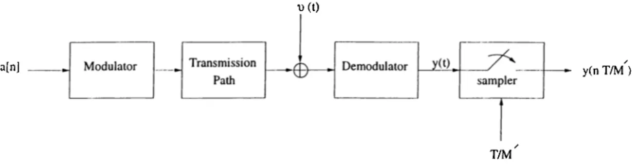
The block-diagram model of a serial transmission system is shown in F'ig. 2.1. In this figure {a[w]}^o input symbol sequence chosen from a finite

al-\)(t)

a[n] _{y(n T/M )}

T/M

Figure 2.1: Model of the communication system.

phabet, y{t) is the received signal and T is the symbol duration. The impulse response of the linear channel, h{t), is the cascade of the transmitter filter, transmission path and the receiver filter. We will assume that h{t) is of finite

duration:

h{t) - O i o r t ^ [ D T , { D + Lh)T) , where D T represents the transmission delay.

(2.1)

Over-sampling of the channel output with a factor of M' provides channel diversity. Consequently as shown in Appendix A, the system in Fig. 2.1 can be equivalently represented as a single-input M '-output discrete-time multi­ channel FIR filter. In the following chapters, we investigate the exact identi­ fication of either all or a subset of these channels. Without loss of generality, assuming that first M < M' of these channels are to be identified, the corre­ sponding multi-channel model is shown in Fig. 2.2. In this figure the outputs of the multi-channel filter are the samples of the received signal y{t):

yi[n] = y{nT + ( ^ - l < i < M . (2.2)

Figure 2.2: Multi-channel filter model.

The FIR filter hc[n] in Fig. 2.2 corresponds to the common zeros of the sub­ channels. If the sub-channels share L\ common zeros, then the length of hc[n] is + 1 . If the sub-channels do not share any common zeros then hc[n] = i[n].

Since all the common zeros are placed in /ic[n], the filters /ii[n],. . . , do not share any common zeros.

The only assumption we make about the model in Fig. 2.2 is that there is no channel noise: u, [n] = 0 for e = 1 ,..., M. Specifically, we state below some of the assumptions and/or constraints that are avoided in our work:

1. The knowledge of the exact channel order as in [8-12].

2. The constraints on the length of the channels and the number of the channels as in [13].

3. The assumption that the sub-channels do not share any common zeros (i.e., hc[n\ — ¿[n]) as in almost every second-order statistics based algo­ rithm [9,12-14]. It has been shown that these algorithms lose their ro­ bustness when this assumption is not true [15]. This is a severe limitation because there exists classes of multi-path communication systems [16,17] for which this assumption is not valid for any over-sampling factor M'. 4. The assumption that the number of sub-channels is the same as the

over-sampling factor.

In Fig. 2.2 we allow the existence of possibly a non-zero delay > 0 as a consequence of (2.1). If at the receiver end the starting time of transmission is known, the delay D can be easily obtained from the observation time of first non-zero channel output. Otherwise, it is impossible to identify the value of D. As will be detailed, even if D is not known, the exact identification of the channels can be carried out.

In this thesis we propose a two stage procedure for the blind-channel- identification (BCI). In the first stage channels h\[n]^. . . , hM[n] are identified. Once, these channels are identified several of the existing algorithms in the literature [18] can be used to estimate the sequence Xc[n] in Fig. 2.2. Then in the second stage, the blind identification of hc{n] is carried out by using the estimated output of this filter Xc[n].

Chapter 3

BLIND IDENTIFICATION OF

THE UNCOMMON ZEROS

In this chapter we set up the framework within which the channels [n],. . . , AmW are identified blindly by using outputs ?/i[n],... ,?/A/[n]. As

shown in Fig. 2.2, the output signals ?/i[n],... are the responses of the channels Ai[n],. . . , AA/[n] to the same input Xc[n]. Thus it can be conjectured that the input-output relationship between pairs of channels might produce sufficient information [12,19] to estimate the channels Ai[n],. . . , without any prior knowledge about the input Xc[n]. In this and the next section we will show that indeed this is the case.

For 1 < i < M, let gi[n] be an estimate of hi[n\. Here we assume that the assumed order ¿ 2 of the channel estimates is larger than or equal to L2 which is the largest order of the channels Aj[nj. Consider two arbitrary and distinct channels, say i and j , in Fig. 2.2. After filtering the outputs of these channels

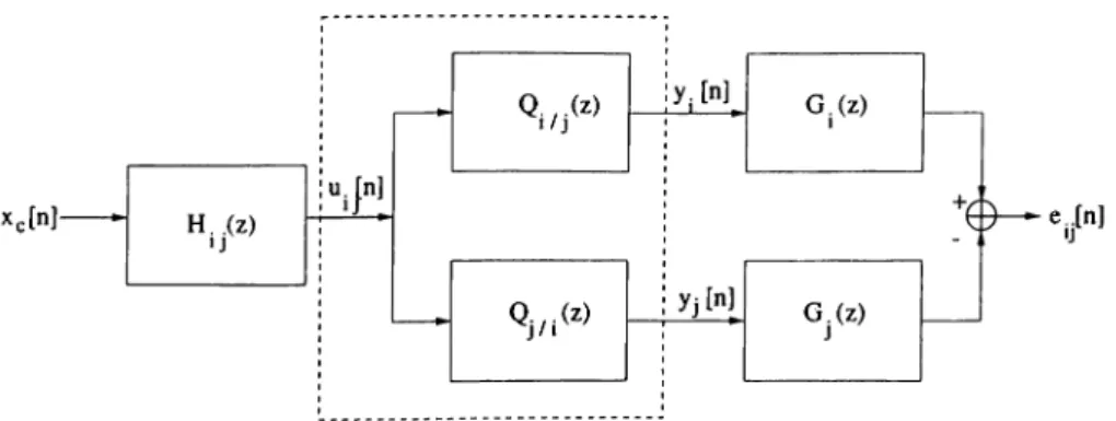
with FIR filters gj[n] and gi[n] we generate the error signal eij[n] as shown in Fig. 3.1.

Figure 3.1: Generation of the error signal e,j[n] associated with the i*·** and sub-channels.

We will base the optimality of a set of channel estimates at the sampling index N of the received data yi[n], I < i < M, to the following cost function:

^ M i - 1

1W) = TT E E i ■ (3-1)

¿=1 j = l

where Jij{gi -,gj ] N)·, the cost function associated with channels i and is defined as: N ^ij{gi ·) gj ) ^ ^ ^ ^ y V - A ; I A;=0 N (3.2) (3.3) = 7 ^ V l^i ^Vj [fc] - 9j [A;] I ^

where Qi and yi[k] are defined as:

^ qAU] (•'^•4)

= yi[k] yi[k - 1] · · · yi[k - ¿2] (•4··^)

Cyj,N in (3.3) is a normalization constant defined as Cw^n = '^N-k and

Wk is a weighting sequence that satisfies

0 < u > i : < l , 0 < k < N

10

We observe that if the channel estimates in Fig. 3.1 are replaced with true chan­ nels, then the cost function in (3.1) becomes identically zero. In other words the true channel coefficients constitute one of the possibly many minimizers of (3.1).

By using (3.4) a more compact representation for the cost Ji^{ g] N) is obtained as:

'^12(9 ‘i ^ ) — 9 ^ ^ y y [ ^ ] 9 1 (3-7) where g is the concatenated channel vector estimates

T

9 = _{9 i} T* ₉₂ T _■■■9Tm

and the hermitian positive semidefinite matrix ilyy[iV] is R ,,[JV ] = F[1V] - Q(1V] , (3.8) (3.9) where and P[AT] = 1 M Ra[ N] 0 0 Ra[ N] 0 0 0 0 M R , [ N ] = ¿=1 ^yi yi [-^] ^yMyi [-^] = J i ^yi y2 [-^] ^yMy2 [-^]

^yi yM [-^] ^yiyM [-^] ^yM yM [-^]

11

(3.10)

(.3.11)

can be interpreted as the weighted cross-correlation matrix of the multi-channel filter outputs yi and yj :

1 ^

Cw,N _fc=o (3.13)

In the following section we will characterize the minimizers of (3.7):

g = a.Tg imn Ry y [ N] g (3.14)

if

3.1

Characterization of the Minimizers of the

Cost Function

In this section, we will present detailed properties of the optimal solutions to the channel identification problem. We begin with the following powerful theorem which states that the optimal solutions are the FIR filtered versions of the actual channel responses.

Theorem 1.

JL2i s ;N) = 0 ^ gi[n] = /i.[n] * /[n] (3.15)

provided that

1) ¿>2 ^

2) TV > Z) + ¿2 H" Z<2

where f[n] is an arbitrary FIR filter of order at most L2 —

Lz-Proof of if part. gi[n] = hi[n] * f[n]

M i - l f - hj *Vi* f\\w,N i=l j = l (3.16) (3.17) 12

M ¿-1

= X ] ^ IK^i * V j — h j * U i) * f \ \ w , N

¿=1 i=i

= 0 ,

where we defined the norm || · \\w,N as ||«||^,Af = ^/Cw,N E L o » « - i l “ WP· a

Proof of only if part. [g ■, N) = 0 iov N > D + L2 + L2 = D + Lr

M 1-1

^ ^ I\9i * V j ~ 9 j * yi\\w ,N — 0

¿=1 j = i

^ Ik' * Vj - 9j * yi\\w,N = 0 , V i j

^ IKfl't * hj Pj * /it ) * ^clIvK.Al ~ fi 1

^ij ·

(

.

)

To complete the proof of the theorem we will make use of several lemmas. In order not to break the continuity of the text, the proofs of the lemmas will be left to appendices.

Lem ma 1. I f IK^rj· * hj — gj * hi) * Xc\\w,n ~ ^ for N > D -\- Lr then gi[n] * hj[n]

—

* /it[n ] =

V n .

This lemma can be used in (3.18) to conclude the equality of gi[n] * hj[n] =

9j[n] * hi[n] for all n. Hence, in the 2-transform domain:

Gi{z)Hj{z) = Gj{z)Hi{z) . (3.19)

Since for i ^ y, Hi{z) and Hj{z) may have common zeros, let monic polynomial Hij{z) be the greatest common divisor of Hi(z) and Hj{z). Hence, H f z ) can be decomposed as:

Hi{z) = Hi,{z)Qi,,{z) (3.20)

where the quotient polynomial Qijj{z) is equal to Hi{z)lHij[z). Then, (3.19) can be written as:

G,(z)H.,(z)Q,ii(z) = G,(z)Hi,(z)Q,i,(z) . (3.21)

After cancellation of the Hij(z) we get;

Gi{z)Qj/.{z) = Gj{z)Qif,{z) . (3.22)

Since, Qj/i{z) and Qi/j{z) have no common zeros;

Qi/,{z)\Gi{z) , V i,i . (3.23)

At this stage we use the following lemma:

Lem ma 2. I f Qi/j{z)\Gi{z) for all i , j then Hi{z)\Gi{z) for all i.

Lemma 2 implies that Gi{z) can be factored as:

Gi{z) = Fi{z)Hi{z) . (3.24)

We complete the proof of the Theorem 1 using the following lemma: Lem m a 3. ^¿(.2:) = Fj{z) for 1 < i , j < M.

This completes the proof of Gi{z) = F[z)Hi{z) for all i. □

Theorem 1 states that the minimizers of (3.7) are FIR filtered versions of the actual /í¿[n]’s where the filter f[n] has length at most L2 — L2 + 1. In the following theorem, the solution space is further characterized.

Theorem 2. The set of vectors 9 = [ g j ■ ■ ■ g ^ V satisfies (3.15) constitutes an + 1 dimensional vector space, where Lc = L2 — L2·

The proof of the theorem is based on the following lemma which will be used to construct a basis for the solution space. The proof of the lemma is given in Appendix E.

L em m a 4. Any vector g in the solution space can he expressed as Lc

9 = Y ^ f [ L c - k]vk , k=Q

where Vk is related to the true channel coefficients as:

Vk = J ’^ _{"at ”}

1 T

/if 0^ I ···

In (3.26) J is a shifting matrix with I ’s on the lower sub-diagonal

0 0 ··· 0 0

1 0

J = 0 1

0 0 and 0 is an Lc dimensional zero vector.

0 0 0 0 1 0 (3.25) (3.26) (3.27)

Proof of Theorem 2. It is easy to see that the vector space assertion holds. In­ deed if ) and ) pairs satisfy the relation (3.25) in Lemma 4, then their linear combination ) + ) also satisfies it. The rest of the theorem is proven by using the Lemma 4 to construct a basis for the solution space.

Based on Lemma 4 we conclude that {vq , . . . , vi^ } constitutes a spanning set for the solution space. Thus the dimension of the solution space is no larger then Zc + 1. We can show that it is exactly Lc + 1 by proving that V k’s are linearly independent. Suppose that otiVi = 0. Then

Vo Vi V2 cto ai C(f = 0 (3.28) 15

Without loss of generality it can be assumed that Uo[0] = /ii[0] is nonzero^ Hence, the above system of equations can be written as:

t^o[0] 0 0 0 X t^o[0] 0 0 X X uo[0] 0 X X X .. uo[0] X X X X «0 ai OL f = 0 (3.29)

which accepts the unique solution of ao = aj = · · · = = 0. Thus V{’s are

linearly independent. □

An important implication of this theorem is stated as:

Corollary 1. The matrix Ryy[ N] has an Lc + I dimensional null-space.

In the next section we will show how the exact identification of /ii[n],. . . , hM[n] can be achieved from a given minimizer of (3.7).

3.2 Identification of

. . . , from

a

Minimizer

of the Cost Function

Suppose that using some optimization algorithm we have computed a particular set of channel estimates ^i[n],... that satisfies (3.15) for some nonzero

hSince /iAi[n] do not share any common zeros, the first coefficient of at least one of these sub-channels should be non-zero.

f[n]. In the following by using the fact that hi[n],. . . , hM[n] do not share any common zeros, we will show how to exactly obtain hi[n],. . . , hM[n] from 9i[n],.. ..,gM[n].

Let’s use the notation 2 { f } to denote the zeros of an arbitrary FIR filter / . Then the zeros of gi[n\ are given as

Z{gi] = Z { f ] U Z { h , ] . (3.30) Since the common zeros of ^¿[^]’s are the zeros of the greatest common divisor of ^¿[n]’s, there exist many algorithms that can be used to obtain them [20]. Formally, these common zeros can be obtained as:

' '¿=1 Z { f } \ J Z { h i } = Z { f } y j [ r \ t , Z { h , ] ] = Z { f ] , (3.31) (3.32) (3.33) where the fact that /ii[n],. . . , hM[n] do not share any common zeros is used in the last step. Hence, we showed that the common zeros of ^,[n]’s are the zeros of f[n\. Thus, we can compute /[n] upto a scaling factor. Finally hi[n] can be found in the ^-domain by polynomial division:

Hi{z) = Gi{z)lF{z) for ¿ = 1 , . . . , M . (3..34) Since, f[n] is not identically zero, the above polynomial division is well defined.

3.3 Constrained Minimization of the Cost

Function

As detailed in the previous section, by starting with an order estimate L2 which is larger than the actual order L2 of channels /ii[n],. . . , /iivi[n], one can obtain a minimizer of the cost function from which the actual channels /ii[n],. . . , /im[w]

are computed by first finding the greatest common divisor and then performing a polynomial division (3.34). Alternatively, by starting with L2 which is larger than ¿2, one can form iiyy[iV] by using (3.9). Then by using Corollary 1, ¿ 2

can be obtained as:

¿2 = -¿2 — i/ + 1 , (3.35)

where 7/ is the dimension of the null-space of . Once the actual order L2 is obtained, the minimization problem (3.14) is solved with ¿ 2 = L2. Since

= L2 — L2 = 0, Theorem 1 states that any minimizer of Jl2{9 ; would be in the form

9i[n] = f[0]hi[n] , fore = l , . . . , M (3.36)

where /[0] is an arbitrary constant. To avoid the undesired trivial solution /[0] = 0, we have to introduce some constraints into the minimization prob­ lem. The constraints should be selected so that they do not alter the global minima of the cost function, but they avoid the above undesired solution. We will investigate the solution to the minimization problem under the following constraints:

(i) 11^ IP = 9 ^

(ii) ll^ilp = /if for some i

(iii) g = a for some fixed vector c .

In the first two, constraints are placed on the energies of the sub-channels. The last one requires the specification of an arbitrary constant c . In the following, closed form solutions of these constrained minimization problems are obtained. Then in Section 3.4 we prove that the minimizers of (3.7) under the constraints (i)-(iii) are identical to the true channel within a multiplicative scale factor.

3.3.1

Energy Constraint 1

Let the eigen decomposition of Ryy be given as^:

M (L 2+1)

■^»1/ = ^ ^ > A2 > · · · > Aa/(^2+i) > 0,

ll^i ||2 = 1 for 1 < i < M{L2 + 1) . (3.37) It is well known that the minimizer of (3.7) under the total energy constraint is the eigenvector of Ryy corresponding to the smallest eigenvalue

9 = liqM(L2+i) · (3.38)

Since Lc = 0, the Corollary 1 states that Ryy has a 1-dimensional null space. Consequently the smallest eigenvalue of Ryy is 0 and its multiplicity is 1.

3.3.2 Energy Constraint 2

Without loss of generality we will assume that the energy constraint is imposed only on to the first channel. Then the constrained optimization problem can

^For notational convenience, the dependence on N is not shown explicitly.

be restated as s.t. rnin Ryy g \\9i \ ? =iA (3.39) (3.40) We partition the matrix Ryy and the vector g as follows:

Ryy — 9 = H ii Ri2 R21 R22 T 9 i -iT T (3.41) (3.42) where jRn = [Ra — Ry^yi )IM. Then the cost function becomes:

«/¿2(5^1 ~ 9 ^ ^ y y 9 (3.43)

— 9\ ^ 1 1 9i + 9\ ^ 1 2 5 R21 9i + ^ 2 2 s

(3.44) We form the lagrangian C

^ 9 i , s , A) = 1 *) + KlA. - \\9i i n and set the gradients of C with respect to g* and s* to zero:

R \ i Ri2 R21 R22 (3.45) 9i = A 9i s 0 (3.46)

In (3.46) R22 cannot be singular, unless g = [0^ g j ■ ■ ■ g j f ]'^ 7^ 0 is a

minimizer of (3.7). However this requires = 0 or 1/1 [n] = 0 V n. In this case the minimization problem should be solved under the constraint ||^i || = 0. However the optimal solution to this constraint minimization problem accepts the trivial solution g = 0 . To avoid this undesired situation, the energy constraint is imposed on a sub-channel which does not have an identically zero

output. Without loss of generality we assume that h\ ^ 0. Therefore (3.46) can be equivalently expressed as

( R l l — jRi2 R22 -^21 ) ^1 —

S = ~ R-22 R-219l

(3.47) (3.48)

Since the hermitian matrix Ryy is nonnegative definite, its Schur comple­ ment, jRii — Rx2 R22 -^21 , is also a nonnegative definite matrix [2 1]. Also A

in (3.47) is an eigenvalue of the Schur complement and gi is the corresponding eigenvector. The ambiguity of which eigenvalue to choose is resolved once it is verified that the substitution of (3.47) and (3.48) into (3.44) yields the mini­ mum of the cost function as A. Consequently we should choose A as the smallest eigenvalue. Thus, the following procedure provides the optimal solution:

1. Find the smallest eigenvalue and the corresponding eigenvector of the Schur complement 2. Normalize gi 3. Compute s { R l l — R i2 R22 ^ 2 1 ) ^ 1 — A m in ^ i 9i - ^ fiig i/W g i S — —R22 ^ 2 1 9l (3.49) (3.50) (.3.51)

Since the dimension of the eigenvalue problem in (3.49) is M times smaller than that of in Section 3.3.1, computationally it is easier to obtain the solution under the second constraint than the first constraint.

3.3.3 Constant Vector Constraint

We know that the unconstrained minimizer of (3.7) is in the null-space of Ryy. If the constant vector c used in this constraint is in the column-space of the hermitian matrix R y y , c G 1Z{Ryy), then g = 0. Therefore the constraint minimization problem should be solved with a = 0. However the minimizer of (3.7) under this constraint accepts the trivial solution g = 0 . To avoid this undesired situation we assume that c ^ 7Z(Ryy ).

We form the lagrangian C:

^ { 9

,

Setting the gradients of C with respect to g* and A* to zero we obtain the following set of equations in g and A:

R'yy 9 — Ac (3.53)

g = a . (3.54)

Since c ^ lZ{Ryy ), (3.53) is inconsistent unless A = 0. If we set A = 0, then (3.53) reads as

9 = , (3.55)

where ^ is an arbitrary complex constant and n is a vector in the \-D null- space of Ryy normalized to have unit norm. Using (3.54) to eliminate ¡5 we obtain the optimal solution as

a 9 =

n n (3.56)

3.4 The Equivalence of the Constrained Solu­

tions

When solving the constrained optimization problems we assumed that = L^, because we can find L2 using the dimension of the null-space of Ryy . On the other hand we know from Theorem 1 that if ¿ 2 = T2, then Jl2(9 ; A^) = 0 if and only ii g is a non-zero multiple of the true channel vector:

9 = /[0]^ , /[0] e C . (3.57)

Therefore to prove that the minimizer of (3.7) under the constraints in Section 3.3 is a non-zero multiple of the true channel, it is sufficient to show that the constrained solutions can be expressed as in (3.57). The following list provides the appropriate multiplicative constants / [0] for each of the optimal solutions:

1. Under the energy constraint 1, choose /[0] = pL/\\h || so that

9 = W II^ II)^ · (3.58)

2. Under the energy constraint 2, choose /[0] = n \l\\h \ || so that

9 = ID* · (3.59)

3. Under the constant vector constraint choose /[0] = a f c ^ h so that

g = ( a l c ^ h ) h . (3.60)

As shown in this section, any of the constraints in Section 3.3 can be used to obtain a non-zero multiple of the true channel when there is no noise in the channel output. However, in the presence of noise, the Theorem 1 does not hold

and the minimization of (3.7) under different constraints in general produces different channel estimates. Currently we are working on the comparison of the channel estimates obtained under the above mentioned constraints when there is noise in the channel outputs.

3.5 A Binary-Tree Algorithm

As shown in the previous section, true channel coefficients can be obtained as the minimizers of (3.7) under the constraints in Section 3.3. Unfortunately, direct computation of the obtained closed form solutions are computationally intensive. For ¿ 2 = 7/2, the direct implementation requires 0{M^L\-{· L \N ) operations for estimation of all the sub-channels /ii[n],. . . , using N con­ secutive channel outputs. In this section we propose to use a binary-tree algorithm to reduce the required computational load to 0 { M L \ + M L \N ).

In order to motivate the idea behind the tree-based algorithm, we first investigate the application of the constrained minimization algorithms to only two arbitrary sub-channels. Suppose that we have the setup shown in Fig. 3.1 and we want to minimize the weighted energy of e,j[„] denoted as Jij{gi ,gj ; N) in (3.3) using one of the constrained minimization algorithms of Section 3.3.

Using the notation in Section 3.1 we denote the common zeros between the and channels as Hij{z). Then Fig. 3.1 can be equivalently rep­ resented as in Fig. 3.2 where the FIR filters Qi/j(z) = Hi{z)lHij{z) and Qj/i{z) = Hj{z)/Hij{z) in this latter figure are coprime. Therefore the esti­ mation of the FIR filters in the dashed box in Fig. 3 .2 is a special case of the

Xc[n]

Figure 3.2: The generation of the error signal tij[n\ associated with the and sub-channels.

M-channel blind identification problem with M = 2. As it is implied by Theo­ rem 1, we can identify Qi/j(z) and Qj/i{z) using exactly Z2+max{Tj/j, Lj/i} + l output samples where T./j is the order of the filter Qi/j{z) and Lj/j is the order of the filter Qj/i(z). The identification of Qi/j{z) and Qj/i{z), can be carried out by using any of the algorithms in Section 3.3. Since these filters do not share any common zeros, their common input u,j[n] can be recovered exactly by using the corresponding 2-channel deconvolution filter. This follows from the Bezout identity [22] which guarantees the existence of a pair of FIR decon­ volution filters Eifj{z), Ej/i{z) of order ma,x{Li/j, Lj/t} such that

(3.61) The deconvolution filters Eiij{z) and Ejii{z) can be computed by using the following partial fraction expansion:

1

___________ ^ Ei/jjz) Ej/i(z) Qiiji^)Qjiii^) Qj/ii^) Qi/A^)

(3.62)

In conclusion, once the FIR filters in the dashed box in Fig. 3 .2 and the FIR filters Ei/j(z) and Ejii{z) in (3.61) are computed the configuration in Fig. 3.3 provides the desired input sequence Uij[n]. This forms the basic idea

u.|n] u jn ] = u.|

The Deconvolution Filter

Figure 3.3: Estimation of the input sequence uq[n].

of the binary-tree algorithm which will be illustrated for M = 4 using the re-arranged multi-channel filter model in Fig. 3.4. In this figure the filters in the dashed boxes 1, 2 and 3 are coprime (see the argument that leads to Fig. 3.2.). Therefore the above results derived for the 2-channel FIR filters can be used to identify the filters in the dashed boxes 1 and 2 and their inputs Ui2[ra] and U34[n]. Since the outputs of the coprime filters Hi2{z) and Hza{z) shown in Fig. 3.4 can be exactly identified, the above results for the 2-channel FIR filters can be used once more to identify these filters together with their common input Xc[n]. This completes the identification of the sub-channels Ai[n],...,/i4[n].

y, [n]

y2W

yjLn]

y.[n]

Figure 3.4: The binary-tree representation of a 4-channel FIR filter.

Chapter 4

BLIND IDENTIFICATION OF

THE COMMON ZEROS

In the previous chapter we have presented a method for blind identification of the sub-channels Ai[n],. . . , /imM in Fig. 2.2 and their common input .Tcfn]. Thus the overall problem is reduced to the blind identification of the filter hc[n] in Fig. 2.2. In this chapter we give a solution to this problem.

We write the input-output relation of the filter hc[n] using the vec- tor/m atrix notation^:

(4.1)

Xc[D] a[0] 0 0 /ic[0]

Xc[D + 1]

= a[l] a[0] 0 hc[i]

Xc[D + L i ] a[ Li ] a [ L i - \ ] ··■· a[0] hc[L,]

®c,il _{A il}

^ Using an over-estimate of does not change the results in this chapter. It only increases the computational load.

In the above equation the vector Xc,Li has been computed as explained in the previous chapter. We also have the a priori information that the information symbols {a[0] , . . . , a[i/i]} which completely determine A i^ are chosen from a finite alphabet A. If the size of this alphabet is J\i then there are only distinct and possible A i^ matrices. Actually depending on the shape of the input symbol constellation this number can be somewhat reduced. For example, if the Binary Phase Shift Keying (BPSK) input symbol constellation is used then the alphabet is ^ = { —1,+1}. In this case it is not possible to distinguish the {Ai^ , h c ) pair from the {—A i^ , —he) pair using only the blind techniques, because both of them satisfies (4.1). However such a constant phase ambiguity is acceptable in digital communications. In practice this phase ambiguity at the receiver can be removed by requiring that the first transmitted information symbol a[0] is always 1.

The algorithm that we propose in this chapter first computes all possible channel estimates that can lead to the output sequence Xc[D]^. . . , Xc[D + L\\. For example, if is one of the possible A i^ matrices then the corre­ sponding channel estimate h^'°^ is obtained by solving (4.1) using the forward- substitution: Af>[01 = Xc[D]/aW[0] 1

'•‘‘VI =

sample index n, the algorithms discards the channel estimates which cannot produce the most recent output sample X c [ n \ . The algorithm terminates when

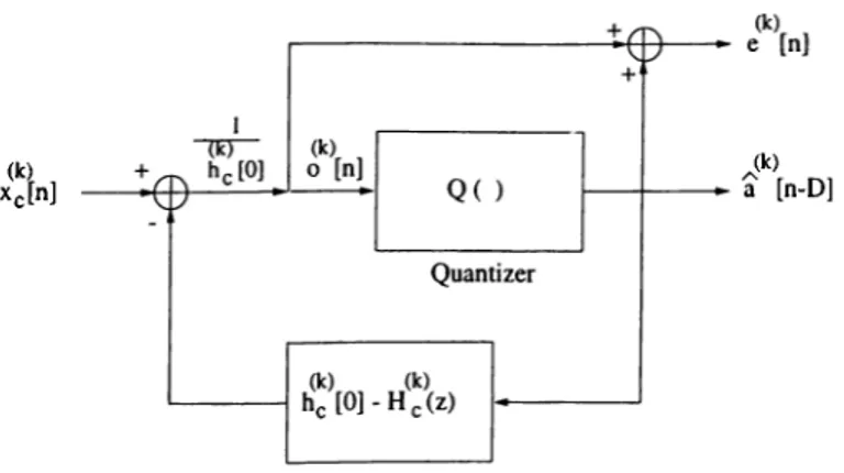
there remains only one channel estimate. After the correct channel is identified using the pruning algorithm, the configuration in Fig. 4.1 provides a solution for the input sequence a[n].

A lgorithm 1 The pruning algorithm Initialization:

Define the current sample index n and the set of remaining channel estimates at the previous sample index:

n — D ~\~ L\ T 1

Pruning loop:

while size(«S(”"^)) > 1 do

Set := .

Compute Xc[n] using the results in Chapter 3. for each channel estimate do

Compute and — D] as in Fig. 4.1. if the residual error

|e<‘>[n|| = |o<‘'[n) - 8<‘>[n - D|| (4.3) exceeds a threshold then

Set := - { h p } . end if

end for

Set n := n + 1 . end while

There exist some pathological cases such that the pruning algorithm does not terminate. In other words there may exist two or more input sequence- channel pairs such that they produce the same output X c [ n \ . Actually this

would always be the case if there were no constraints on the input sequence. But in the context of digital communications the samples of the input sequence (i.e., the information symbols) are chosen from a finite alphabet A with M

XcW a [n-D]

Figure 4.1: Identification of the common zeros.

elements. Unfortunately even under such a stringent constraint there exists such pathological cases. For example consider the following input sequence and channel pairs:

(α^[n],/¿cı[n]) = ((-l)"w [n],i[n] + ¿[n - 1]) (4.4) (a2[n],/icjn]) = (u[n],6[n] - (Ç[n - 1]) . (4.5) A straightforward calculation shows that Xcjn] = Xc2[>t] = <^[^]· Thus knowing

only the output sequence Xc[n] = <^[n] it is impossible to tell which input se­ quence has been actually transmitted^. So this identifiability problem applies to all blind channel identification algorithms.

The above discussion proves the existence of input sequence-channel pairs which produce the same output. However in practice what is important is the probability of coming across to such pathological cases. Now we show that this probability is zero.

Theorem 3. Suppose that the output sequence Xc[n\ which is not identically zero is observed for n > 0. The vectors of filter coefficients

he — /ic[0] hc[l] ··· hc[Li (4.6)

^Notice that there was no identifiability problem in estimation of the uncommon zeros.

which produce the output Xc[n] for a suitable input sequence a[n] are isolated points in Li + I dimensional space.

Proof. The proof is by contradiction. Let e > 0 be given. Then there exists Li + 1 dimensional vectors hci , hc^ such that

0

llh’ci

h.c

I I ^

X,{z) = z - ^ A , {z)HcA^) = z->^A.i{z)H,,{z) .- D (4.8)

Let Hc^iz) = Hci(z) +6Hc{z), ^2(2) = Ai(z) + 6A{z). Substituting these into (4.8) yields:

H ,,{ z )8A { z ) p8H ,{z)A,{z) + 8H ,{z )8A{z) = 0 . (4.9) In this equation, Hc^{z) is fixed, 8A{z) is the 2-transform of a sequence whose samples can take values only the in the set {—2, —1 ,0 ,1,2), and 8Hc{z) is an arbitrary FIR filter. Let e —> 0 in (4.7). Then (4.9) reads as

Hc,{z)8A{z) = 0 . (4.10)

Since 8A{z) 7^ 0 (because Hc^{z) ^ Hc2{z) in (4.8)), the above condition can be satisfied only if Hd{z) — 0. Then, it follows from (4.8) that Hc.^(z) = 0. /1

contradiction. □

As a consequence of this theorem we conclude that the measure of such pathological input sequence-channel pairs is zero among all admissible pairs.

^For simplicity we assume that the input sequences are drawn from a BPSK symbol constellation.

Therefore in practice the pruning algorithm always identifies hc[n] in a finite number of iterations. As shown in the next chapter when the common zeros are identifiable from Xc[n\ the pruning algorithms converges to the solution very fast. On the other hand if the identification of the common zeros is desired under all circumstances, then the transmission of a known initialization sequence of length Li + l should be tolerated so that (4.1) can be solved for the common zeros hc[n\. Note that unlike a training sequence which is transmitted periodically, the initialization is performed only once.

Chapter 5

SIMULATION

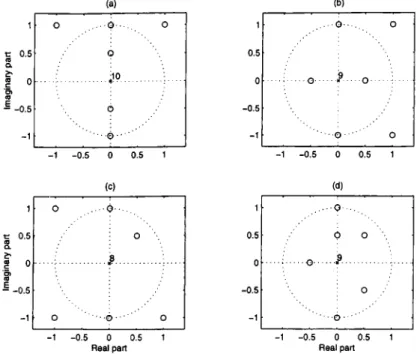
In this chapter an illustrative simulation is presented to highlight the order of the operations used in BCI problem. Consider the 4-channel FIR system {M = M ' = 4) with the pole-zero plots shown in Fig. 5.1. Each pair of channels in this figure share exactly 3 common finite zeros, where the two of these zeros are common to all of the 4 channels (i.e, Hfiz) = 1 + The delay associated with a particular channel is given as the number of the zeros of that channel at infinity^, which can found in Fig. 5.1 as the difference between the number of poles at the origin and the number of finite zeros. For example the delay associated with the first channel is 10 — 6 = 4 samples. Similarly the delays associated with the other channels are 3, 2 and 3 samples respectively.

The FIR system with these pole-zero plots can be decomposed into a binary-tree structure as shown in Fig. 3.4. It is known that such a decompo­ sition is always ambiguous upto constant scale factors. For example consider

^Except for this discussion, we will not discriminate between the finite zeros and the zeros at infinity (delays).

multiplying all the filters in the dashed boxes 1 and 2 by a non-zero 7 G C and multiplying all the filters in the dashed box 3 by I /7 . To remove this ambiguity we will scale the filters in Fig. 3.4 such that the first non-zero samples of the filters except for those at the leaves (dashed boxes 1 and 2) are always 1.

The first box in Fig. 3.4 is the overall delay D — 2 oi the communication system which is defined as the minimum of the delays of each sub-channel. The filter Hc{z) = 1 + z~'^ in this figure represents the common finite zeros to the 4

channels, Hij{z), i j , denotes the zeros common to the and channels apart from those in z~^Hc{z) and finally Qijfizfi i ^ j , denotes the zeros of the channel which are not also in the channel. The importance of this representation is that the filters in a dashed box do not share any common zeros. For example the zeros common to and 2"*^ channels are in z~^Hc{z)H\2{z) therefore Q \i2{z) and <5 2/1(2) cannot have any zeros in common.

In this simulation, the independent identically distributed input sequence a[n] is drawn from a BPSK symbol constellation, hence the causal input se­ quence consists of - |- / - l ’s for n > 0.

5.1 The Estimation of the Delay

The outputs ?/i[n],. . . , i/4[n] of the channels are shown in Fig. 5.2. We use this figure to identify the delays associated with the channels. For example we observe that yi[n] = 0 for n < 4 and yi[4] ^ 0. Thus the delay associated with the first channel is 4 samples. With similar reasoning the delays associated with other channels are found as 3, 2 and 3 samples z'espectively. Finally we compute the common delay of the communication system a,s D — min{4,3,2,3} = 2.

5.2 The Binary-tree Algorithm

The next step is the identification of the filters in the boxes labeled as 1, 2 and 3 in Fig. 3.4 (the binary-tree of section 3.5). We will first estimate the leaves of the tree (boxes 2, 3) and finally the root (box 1). The following comments refer to the computation of the FIR filters Q\i2{z) and (^2/i(^) in box 1 and their common input Ui2[n\.

1) The data in Fig. 5.2 is used. Therefore N = 20. 2) The filter orders are overestimated as L2 = 8.

3) The matrix f?j,y[Ar] in 13.9) is computed with M = 2 and Z2 = 8 using t/i[n] and j/2[n], 0 < n < iV. The singular values of ilyy[iV] are plotted in Fig. 5.3. Clearly 7/, the number of zero singular values, is 5.

4) The maximum of the orders of Q\f2{z) and Q2i\{z) is computed as L2 =

¿ 2 — 77 + 1 = 4.

5) Ryy[N] is recomputed using the true filter order L2 = 4. Any of the constrained minimization algorithms of Section 3.3 can be used to com­ pute the estimates Qi/2{z) and Q2/i{z) from /2yy[iV]. In this example, Energy Constraint 1 is used to compute Qi/2{z) and (^2/1 (^) as:

Qi/2{z) = (-0.37403 - 0.13025i)gi/2(^)

Q2/i{z) = (-0.37403 - 0.13025i)g2/i(-^) ·

(5.1) (5.2)

6) The FIR deconvolution filters E if2{z) and E2/i{z) are computed using (3.62). The output of the deconvolution filters is computed as (see

Fig. 3.3)

ui2[n] = (-2.3844 + 0.83038;)ui2[n] , 0 < n < . (5.3)

Adapting the same steps to the 2"^* box, we identified the filters in the 2"*^ box and their common input U34[ra] for 0 < n < A/^ as

QzIa{z) = ( - 0 .2 4 9 2 7 ) ( 5 3 / 4 ( ^ ) ( 5 .4 )

Qa!z{z) = ( - 0 . 2 4 9 2 7 ) g 4 / 3 ( ^ ) ( 5 .5 ) «34 [n] = ( - 4 . 0 1 1 7 )w3 4 M · ( 5 .6 )

At this point we know the output of the filters in the 3’’'* box, Ui2[n] and U34[n], for 0 < n < A^ which is sufficient to estimate Hi2{z) and H2,a{z). The

estimates of these filters and their common input 0 < n < A^ are found as Hu{z) = (0.064595 + 0.37838i)^i2 (2) = (-0.10080 + 0.60151i)/f34(-^) Xc[n] = (1.0871 +6.4872j)a:,[n] . (5.7) (5.8) (5.9)

5.3 The Pruning Algorithm

The last problem is the identification of Hc{z) in Fig. 3.4 from its estimated output Xc[n]. This is accomplished using the pruning algorithm of Chapter 4. In this example we overestimate the number of common zeros as L\ = 4. We note that for 0 < n < 4 there are only 32 possible input sequences

half of which differ only in sign. Therefore there are effectively only 16 non

trivially distinct input sequences. Since Xc\n]^ the output of the filter Hc{z), has been already identified, we use (4.2) to compute the 16 channel estimates corresponding to each of the distinct input sequence Then for each channel estimate we compute the residual error n > Z ) + Ti + l = 7, defined in Chapter 4. The running energy of the residual errors

¿54") = ' (5.10)

j= 0

for all the channel estimates are plotted in Fig. 5.4. In this figure we see that the energy of only one of the error sequences remains around at all samples. Hence this channel is identified as the estimate of the common zeros,

Hc(z) = (1.0871 + 6.4872;)/i42) . (5.11) The use of Hc{z) in Fig. 4.1 provides the estimate of the input sequence

a[n] — a[n] . (5.12)

(0 c S’ E (a) (b) 1 O o 1 o 0 .5 ₉ 0 .5 0...; ...c\.... 9 . . . . Q ... ... - 0 . 5 6 - 0 . 5 - 1 - 1 0 o - 1 - 0 . 5 0 0 .5 1 - 1 - 0 . 5 0 0 .5 1 (c) (d) 1 o 1 0 .5 o ■. 0 .5 0 o ■·. 0...: ... ... 0 -0 .5 - 0 . 5 O - 1 o 0 - 1 •■■•o· ·■ - 1 - 0 . 5 0 R e a l p art 0 .5 1 - 1 - 0 . 5 0 R e a l p art 0 .5 1

Figure 5.1: The pole-zero plots of the channels: (a) Channel 1, (b) Channel 2, (c) Channel 3, (d) Channel 4. 10 1 6 .t; s> 2 4 2 (b ) I k (c) O H D O O ‘ 0 5 10 15 2 0 s a m p le (d) 1.2D> CO 2 1 ■eee-0 5 10 15 2 0 s a m p le

Figure 5.2: The magnitudes of the outputs of the channels: (a) Channel 1, (b) Channel 2, (c) Channel 3, (d) Channel 4.

Figure 5.3: The singular values.

Figure 5.4: The running energy of the error sequences associated with different channel estimates (identification of the common zeros).

Chapter 6

CONCLUSIONS

The blind channel identification problem is investigated using the multi­ channel filter model of the communication system. The main contribution of this thesis is to give the exact solution to this problem under the noise-free case virtually with the least set of constraints on the channel. Furthermore this is achieved based on a very short observation of the channel output sequence. This is an important result because the current algorithms in the literature are in general either fast converging to the solution but applicable to only a certain restricted class of channels (SOCS-based algorithms) or generally ap­ plicable but computationally intensive and large amount of data demanding (HOS-based algorithms).

In this thesis the problem is divided into two sub-problems which are in­ dependently formulated and solved: The identification of the uncommon zeros (i.e., hi[n],. . . , hM[n]) followed by the identification of the common zeros (i.e., hc[n]) in the multi-channel filter model. The first sub-problem is formulated

in Chapter 3. In that chapter a cost function in terms of the sub-channels h\[n],. .. ,hM[n] is derived and its minimizers are fully characterized with a powerful theorem. An important aspect of this theorem is that it also specifies the minimum number of samples required for the exact identification of the sub-channels . . . , upto a scalar multiplicative constant. Based on this theorem several closed-form solutions are provided to estimate these sub­ channels and the equivalence of these estimates under the noise-free case is proven. The investigation of the behavior of these closed-form solutions under the more realistic noisy channels is a future research topic. Finally a novel binary-tree algorithm is provided to estimate these channels in a computation­ ally efficient way. The utilization of this structure in noisy channels is also a future research topic.

The solution to the second sub-problem, i.e., the identification of the filter hc[n] corresponding to the common zeros, is given in Chapter 4 based on a novel pruning algorithm. This algorithm first identifies all possible estimates of hc[n] based on first few samples of the output. This is achieved using the fact that the input symbols are not arbitrary but drawn from a known symbol constellation. The basic step of the algorithm is to eliminate the channel estimates which are inconsistent with the observation of the current output sample. If the BCI problem is solvable then the pruning algorithm always converges to the true solution in a finite number of steps. It is shown with simulation that this algorithm is practical for moderate orders of hc[n] and in practice it converges to the true solution very fast.

Bibliography

[1] S. Haykin, Adaptive Filter Theory. New Jersey: Prentice-Hall, third ed., 1996.

[2] Y. Sato, “A method of self-recovering equalization for multi-level am­ plitude modulation,” IEEE Trans, on Communications, vol. COM-23, pp. 679-682, June 1975.

[3] A. Benveniste, M. Goursat, and G. Rüget, “Robust identification of a nonminimum phase system: Blind adjustment of a linear equalizer in data communications,” IEEE Trans. Automatic Control, vol. COM-25, pp. 385-399, June 1980.

[4] D. N. Godard, “Self-recovering equalization and carrier tracking in two dimensional data communication systems,” IEEE Trans, on Communica­ tions, vol. COM-28, pp. 1867-1875, 1980.

[5] G. Picci and G. Prati, “Blind equalization and carrier recovery using a “stop-and-go” decision-directed algorithm,” IEEE Trans, on Communi­ cations, vol. COM-35, pp. 877-887, 1987.

[6] Y. Li and Z. Ding, “Convergence analysis of finite length blind adaptive equalizers,” IEEE Trans. Signal Process., vol. 43, pp. 2120-2129, Sept.

1995.

[7] D. R. Brillinger, Time Series: Data analysis and theory. New York: Holt, Rinehart, and Winston, 1974.

[8] L. Tong, G. Xu, and T. Kailath, “Blind identification and equalization based on second-order statistics: A time domain approah,” IEEE Trans. Information Theory, vol. 40, pp. 340-349, Mar. 1994.

[9] G. B. Giannakis and S. D. Halford, “Blind fractionally spaced equalization of noisy FIR channels: Direct and adaptive solutions,” IEEE Trans. Signal Process., vol. 45, pp. 2277-2292, Sept. 1997.

[10] E. Moulines, P. Duhamel, J. F. Cardoso, and S. Mayrargue, “Subspace methods for the blind identification of multichannel FIR filters,” IEEE

Trans. Signal Process., vol. 43, pp. 516-525, Feb. 1995.

[11] D. T. M. Slock, “Blind fractionally-spaced equalization, perfect recon­ struction filter banks and multi-channel linear prediction,” in Proc. IEEE Int. Conf. Acoust. Speech Signal Process., vol. 4, pp. 585-588, 1994. [12] G. Xu, H. Liu, L. Tong, and T. Kailath, “A least-squares approach to blind

channel identification,” IEEE Trans. Signal Process., vol. 43, pp. 2982- 2993, Dec. 1995.

[13] H. Liu and G. Xu, “Closed-form blind symbol estimation in digital com­ munications,” IEEE Trans. Signal Process., vol. 43, pp. 2714-2723, Nov. 1995.

[14] D. Gesbert, P. Duhamel, and S. Mayrargue, “On-line blind multichannel equalization based on mutually referenced filters,” IEEE Trans. Signal Process., vol. 45, pp. 2307-2317, Sept. 1997.

[15] A. Touzni and I. Fijalkow, “Robustness of blind fractionally-spaced iden- tification/equalization to loss of channel disparity,” in Proc. IEEE Int.

Conf. Acoust. Speech Signal Process., pp. 3937-3940, 1997.

[16] Z. Ding, “Characteristics of band-limited channels unidentifiable form second-order cyclostationary statistics,” IEEE Trans. Signal Processing Letters, vol. 3, pp. 150-152, May 1996.

[17] J. Tugnait, “On blind identifiability of the multipath channels using frac­ tional sampling and second-order cyclostationary statistics,” IEEE Trans. Information Theory, vol. 41, pp. 308-311, Jan. 1995.

[18] B. Farhang-Boroujney, “Channel equalization via channel identification: Algorithms and simulation results for rapidly fading HF channels,” IEEE

Trans, on Communications, vol. 44, pp. 1409-1412, Nov. 1996.

[19] M. I. Gürelli and C. L. Nikias, “Evam: An eigenvector-based algorithm for multichannel blind deconvolution of input colored signals,” IEEE Trans. Signal Process., vol. 43, pp. 134-149, Jan. 1995.

[20] W. Qui and Y. Hua, “A GCD method for blind channel identification,” Digital Signal Processing, pp. 199-205, 1997.

[21] L. L. Scharf, Statistical signal processing detection, estimation, and time series analysis, ch. 2. Addison-Wesley, 1991.

[22] T. Kailath, Linear Systems. New Jersey: Prentice-Hall, 1980.

APPENDIX A

Multi-channel Filter Model

The fact that the channel model in Fig. 2.1 can be represented as in Fig. 2.2 is widely used in the current blind channel identification literature. Here we provide a proof of this result.

The filtered and noise corrupted received signal y{t) is given as

OO

2/(0 = Y , a[m\h{t — m T ) v { t ) , (A.l) m = 0

where h{t) is the baseband model of the channel defined in Chapter 2 and u(i) is the additive channel noise. The output of the sampler in Fig. 2.1 is the samples of y{t) taken at an M ' times faster rate then the baud rate. It is given as r p ^ r r \ r j l ^ (A.2) rp rp rp 771=0 M " ₇₇₁₌₀^ ^ ‘ ^ M' ' - M' Substituting k — nM ' + (t — 1) into (A.3) it turns out that

rp OO rp rp

y{nT + { i - l ) — ) = Y a [ m ] h { { n - m ) T + { i - l ) — ) + v { n r + { i - l } — )

771=0

fori = l , . . . , M ' (A.3)