New solution methods for single machine bicriteria scheduling problem : minimization of average flowtime and number of tardy jobs

NEW SOLUTION METHODS FOR SINGLE MACHINE

BICRITERIA SCHEDULING PROBLEM: MINIMIZATION OF

AVERAGE FLOWTIME AND NUMBER OF TARDY JOBS

A THESIS

SUBMITTED TO THE DEPARTMENT OF INDUSTRIAL ENGINEERING AND THE INSTITUTE OF ENGINEERING AND SCIENCE

OF BILKENT UNIVERSITY

IN PARTIAL FULFILLMENT OF THE REQUIREMENTS FOR THE DEGREE OF

MASTER OF SCIENCE

By

Fatih Safa Erenay July, 2006

I certify that I have read this thesis and that in my opinion it is fully adequate, in scope and in quality, as a thesis for the degree of Master of Science.

Prof. İhsan Sabuncuoğlu (Principal Advisor)

I certify that I have read this thesis and that in my opinion it is fully adequate, in scope and in quality, as a thesis for the degree of Master of Science.

Asst. Prof. Ayşegül Toptal

I certify that I have read this thesis and that in my opinion it is fully adequate, in scope and in quality, as a thesis for the degree of Master of Science.

Prof. Erdal Erel

Approved for the Institute of Engineering and Science:

Prof. Mehmet Baray

Abstract

NEW SOLUTION METHODS FOR SINGLE MACHINE BICRITERIA SCHEDULING PROBLEM: MINIMIZATION OF AVERAGE FLOWTIME AND

NUMBER OF TARDY JOBS

Fatih Safa Erenay M.S. in Industrial Engineering Supervisor: Prof. İhsan Sabuncuoğlu

July 2006

In this thesis, we consider the bicriteria scheduling problem of minimizing number of tardy jobs and average flowtime on a single machine. This problem, which is known to be NP-hard, is important in practice as the former criterion conveys the customer’s position and the latter reflects the manufacturer’s perspective in the supply chain. We propose two new heuristics to solve this multiobjective scheduling problem. These two heuristics are constructive algorithms which are based on beam search methodology. We compare these proposed algorithms with three existing heuristics in the literature and two new meta-heuristics. Our computational experiments illustrate that proposed heuristics find efficient schedules optimally in most of the cases and perform better than the other heuristics.

Keywords: Bicriteria Scheduling, Average Flowtime, Number of Tardy Jobs, Beam Search.

Özet

TEK MAKİNEDA İKİ ÖLÇÜTLÜ ÇİZELGELEME PROBLEMİ İÇİN YENİ ÇÖZÜM METODLARI: ORTALAMA AKIŞ SÜRESİ VE TOPLAM GEÇ KALMIŞ

İŞ SAYISINI ENKÜÇÜKLEME

Fatih Safa Erenay

Endüstri Mühendisliği Yüksek Lisans Tez Yöneticisi: Prof. İhsan Sabuncuoğlu

Temmuz 2006

Bu tezde, ortalama iş akış süresini ve toplam geç kalmış iş sayısını enküçüklemeyi hedefleyen iki ölçütlü tek makina çizelgeleme problemini ele aldık. NP-zor olduğu bilinen bu problemın önemi ele aldığı ölçütlerden kaynaklanmaktadır. Zira, ele alınan birinci ölçüt tedarik zinciri içerisindeki bir üreticinin, ikincisi ise bir tüketicinin bakış açısını temsil eder. Bu çok ölçütlü problem için iki yapıcı sezgisel yöntem öneriyoruz. Bu iki yöntem ışın taraması algoritması esas alınarak geliştirilmiştir. Önerilen bu iki algoritma, üçü literatürde mevcut ikisi de yeni geliştirilmiş olan, 5 farklı sezgisel yöntem ile karşılaştırılmıştır. Yaptığımız sayısal testler sonucu, önerdiğimiz algoritmaların, çoğu zaman en iyi etkin çizelgelere ulaştığı ve karşılaştırıldıkları sezgisel yöntemlerden daha iyi sonuçlar verdikleri tesbit edilmiştir.

Anahtar Kelimeler: İki Ölçütlü Çizelgeleme, Ortalama İş Akış Süresi, Toplam Geç Kalmış İş Sayısı, Işın Taraması.

Acknowledgement

I would like to express my sincere gratitude to Prof. İhsan Sabuncuoğlu and Asst. Prof. Ayşegül Toptal for their instructive comments and encouragements in this thesis work. I believe that their valuable suggestions in the supervision of the thesis will guide me throughout all my academic life.

I am indebted to Prof. Erdal Erel for accepting to review this thesis, and his useful comments and suggestions.

I would like to express my special thanks to Süleyman Kardaş and Mustafa Aydoğdu for their computational aids, sharing their technical knowledge with me and for their friendship.

I am also indebted to Prof. Selim Aktürk, Assoc. Prof. Oya Ekin Karaşan, Asst. Prof. Emre Alper Yıldırım, and Asst. Prof. Mehmet Rüştü Taner for their valuable time and feedbacks.

I would also like to thank to Selçuk Gören, Hakan Gültekin, Mehmet Mustafa Tanrıkulu, Muzaffer Mısırcı, Fazıl Paç, Gülay Samatlı, Ahmet Camcı, Cağdaş Büyükkaramıklı, Çagrı Latifoğlu, Sinan Gürel, Ayşegül Altın, Sıtkı Gülten and my other friends for their helps and morale support during my graduate study. Finally, I would like to express my deepest gratitude to my family for their understanding and patience during my graduate life.

CONTENTS CHAPTER 1 ...…………. …. 1 INTRODUCTION ...….….. …. . 1 CHAPTER 2 ...….….. ………... 3 LITERATURE REVIEW ...…… 3 CHAPTER 3 ... 6 PROBLEM FORMULATION………... 6 CHAPTER 4 ... 10

OPTIMAL SOLUTION METHODOLOGY FOR MINIMIZING n_T AND F …. 10

CHAPTER 5 ... 13

PROPOSED BEAM SEARCH ALGORITHMS AND OTHER HEURISTICS 13 5.1. Independent Beam Search (BS-I) ………... 14

5.2. Dependent Beam Search (BS-D) ..………... 15

5.3. Genetic and Tabu-search Algorithms (GA and TS) ... 15

CHAPTER 6 ... 16

COMPUTATIONAL EXPERIMENTS ... 16

6.1. Comparison with the Optimum Solution …... 17

6.2. Experiments on Larger Problems………... 25

CHAPTER 7 ... 31

BIBLIOGRAPHY ... 33

LIST OF FIGURES

FIGURE 1: AVERAGE PERCENTAGE DEVIATION VS BEAM WIDTH... 18 FIGURE 2: B&B TREE FOR THE SAMPLE PROBLEM ………... 38 FIGURE 3: INDEPENDENT BEAM SEARCH TREE FOR THE SAMPLE PROBLEM... 41

FIGURE 4: DEPENDENT BEAM SEARCH TREE FOR THE SAMPLE PROBLEM... 43

LIST OF TABLES

Table 1: Sample problem parameters………... 37 Table 2: Due date ranges for the test problem ………... 16 Table 3: Comparison of the heuristics with the optimum solution ………... 21 Table 4: Average deviation from optimum in the problems with low processing variability……… 23

Table 5: Average deviation from optimum in the problems with high processing

variability……… 24

Table 6: Number of efficient schedules for which no solution is found ……... 25 Table 7: Comparison of the other heuristics with Nelson’s Heuristic .…... …... 28 Table 8: Number of efficient schedules for which no solution is found …...….. 30 Table 9: Average CPU time in milliseconds ……..……….. 30 Table 10: Comparison of heuristics with optimum solution on the test problems with 20 jobs and low processing time variability……….………. 52

Table 11: Comparison of heuristics with optimum solution on the test problems with 20 jobs and high processing time variability ….……… 53

Table 12: Comparison of heuristics with optimum solution on the test problems with 30 jobs and low processing time variability …..……… 54

Table 13: Comparison of heuristics with optimum solution on the test problems with 30 jobs and high processing time variability ….……… 55

Table 14: Comparison of heuristics with optimum solution on the test problems with 40 jobs and low processing time variability …..……… 56

Table 15: Comparison of heuristics with optimum solution on the test problems with 40 jobs and high processing time variability ….……… 57

Table 16: Comparison of heuristics with optimum solution on the test problems with 60 jobs and low processing time variability …..……… 58

Table 17: Comparison of heuristics with optimum solution on the test problems with 60 jobs and high processing time variability ….……… 59

Table 18: Comparison of heuristics with Nelson’s Heuristic on the test problems with 80 jobs and low processing time variability ………... ……….. 61

Table 19: Comparison of heuristics with Nelson’s Heuristic on the test problems with 80 jobs and high processing time variability ……….. ……….. 62

Table 20: Comparison of heuristics with Nelson’s Heuristic on the test problems with 100 jobs and low processing time variability ..……... ……….. 63

Table 21: Comparison of heuristics with Nelson’s Heuristic on the test problems with 100 jobs and high processing time variability ……….. ……… 64

Table 22: Comparison of heuristics with Nelson’s Heuristic on the test problems with 150 jobs and low processing time variability ……….……….…….. 65

Table 23: Comparison of heuristics with Nelson’s Heuristic on the test problems with 150 jobs and high processing time variability …………...….……….….. 66

C h a p t e r 1

INTRODUCTION

In the literature most scheduling studies consider optimization of a single objective function. However, in practice, decision makers evaluate schedules according to more than one measure. Since using multiple criteria is more realistic, several multicriteria scheduling papers have appeared in the scheduling literature. Most of these papers are on single machine bicriteria scheduling problems. In the vein of this literature, this thesis study considers minimization of mean flowtime ( F ) and number of tardy jobs (nT) on a single machine. Our contribution lies in

developing new heuristics that outperform the current approximate solution methodologies. Also, we characterize the effectiveness of these proposed heuristics in terms of problem parameters.

We propose two heuristics, which are constructive algorithms based on beam search method. In addition, two heuristics iteratively utilizing genetic algorithm and tabu-search are developed by Kardas and Sabuncuoglu (2006) and Aydogdu and Sabuncuoglu (2006). These new heuristics are designed to find the approximately efficient schedules. That is, they can estimate the pareto frontier solutions for the problem of minimizing mean flowtime ( F ) and number of tardy jobs (nT) on a single machine.

Efficient schedules are the set of schedules that cannot be dominated by any other feasible schedule according to the considered criteria. All other schedules, which are not in this set, are dominated by at least one of these efficient schedules. The reason for seeking efficient schedules instead of minimizing weighted sum of

nT and F is that whatever the weights are, the optimum solution will be one of the

efficient schedules. Specifically, given the efficient schedules for the bicriteria problem and the corresponding weights w1 and w2, the solution to the

minimization of w1 F + w2 nT can be found by evaluating all these finite number

of efficient schedules.

Number of tardy jobs and average flowtime are quite significant criteria for characterizing the behavior of a manufacturer who wants to meet the due dates of his/her customers while minimizing own inventory holding costs. The solution to the single machine problem which is known to be NP-hard (Bulfin and Chen, 1993) can be used as an aggregate schedule for the manufacturer, or for generating a more detailed schedule for a factory based on a bottleneck resource. Thus, having an effective approximate solution methodology for finding efficient schedules to this problem is important both theoretically and in practical sense.

The organization of this thesis is as follows. In Section 2, we present a literature review on multicriteria scheduling. In Section 3, we formulate the problem of minimizing number of tardy jobs and average flowtime on a single machine. In Section 4, we describe Nelson et al. (1986)’s optimum solution method for this problem. The proposed beam search algorithms are presented in Section 5. Computational results are provided in Section 6. Finally, concluding remarks and future research directions are given in Section 7.

C h a p t e r 2

LITERATURE REVIEW

In the scheduling literature, most of the studies consider bicriteria single machine scheduling problems that minimize couples of criteria such as maximum tardiness and flowtime (Smith, 1956; Heck and Robert, 1972; Sen and Gupta, 1983; Koksalan, 1999), maximum earliness and flowtime (Koksalan et al., 1998; Koktener and Koksalan, 2000; Keha and Koksalan, 2003), maximum earlinessand number of tardy jobs (Erol et al., 1998; Kondakci et al., 2003). Extensive surveys of several bicriteria single machine scheduling studies are provided by Dileepan and Sen (1988), Fry et al. (1989) and Wan and Yen (2003). In addition to these survey papers, Nagar et al. (1995), Billaut and T’kindt (1999) and Hoogeveen (2005) review multicriteria scheduling literature including those papers that consider more than two criteria and more complex settings.

Bulfin and Chen (1993) analyze the complexity of the single machine multicriteria scheduling problems which consider maximum tardiness, flowtime, number of tardy jobs, tardiness and the weighted counterparts of the last three criteria. A more recent publication that reviews the complexity of the multicriteria scheduling problem is by T’kindt et al. (2005). The paper is mainly about the enumeration complexity theory. Nevertheless, the survey also reviews the complexity of several multicriteria scheduling problems as an application of the theorems presented in the paper.

Multicriteria scheduling studies can be grouped into three categories as: hierarchical optimization, weighted sum optimization and pareto optimization

(Wan and Yen, 2003). Hierarchical optimization approach tries to minimize some of the criteria while keeping the others at their optimal value. In weighted sum optimization approach, the decision makers assign weights to the criteria. Thus, the multiple criteria are reduced to a single performance measure. The last category, pareto optimization, minimizes corresponding criteria simultaneously by finding efficient schedules. The current study belongs to the last category.

For single machine case, the problem of minimizing nT, while F is optimum,

is solved in polynomial time (Chen and Bulfin, 1993) by an adjusted version of SPT order which applies Moore’s Algorithm to break ties among the jobs with equal processing time. In the rest of the thesis, SPT order will refer to this adjusted version. In another study, Emmons (1975) develops an algorithm for minimizing

F while nT is optimum. Later, this problem is showed to be NP-Hard by Huo et

al. (2005). Finally, Chen and Bulfin (1993) prove that simultaneously minimizing both criteria on a single machine via finding efficient schedules is NP-Hard.

Then, Nelson et al. (1986) develop a branch and bound procedure to find efficient schedules for minimizing nT and F optimally on single machine. In

addition, Nelson et al. (1986) develop a constructive heuristic for this problem. In another study, Kiran and Unal (1991) define several theorems about the characteristics of the efficient solutions. Kondakci and Bekiroglu (1997) present some dominancy rules on the efficient solutions, which they use to develop more effective optimal solution method. These dominancy rules are applied to the Nelson et al.’s branch and bound procedure. Consequently, the paper reports that the size of branch and bound tree is reduced considerably.

Recent studies on the problem propose some general purpose procedures. Koktener and Koksalan (2000), and Keha and Koksalan (2003) develop heuristic methods based on simulated annealing and genetic algorithms, respectively. The later study indicates that genetic algorithm generally performs better than the

simulating annealing; however, simulating annealing approach is faster than the genetic algorithm.

After reviewing these studies we observe that there are many multicriteria scheduling papers in the literature. However, only a few solution methodologies, (one exact and three heuristics) are proposed for the problem that the current study considers. Moreover, these solution methods are not compared with each other in detail. Thus their relative strengths are unknown. Only simulated annealing (Koktener and Koksalan, 2000) and genetic algorithm (Keha and Koksalan, 2003) approaches are compared with each other. Nevertheless, these two iterative methods are not properly compared with the optimum solution for problems with more than 20 jobs. Therefore, the current study presents two constructive and two iterative heuristic methods for this problem and compares these proposed heuristics with each other as well as with the other exact and heuristic solution methods available in the literature. Hence, the current study will illustrate the relative strengths of each solution method.

C h a p t e r 3

PROBLEM FORMULATION

As discussed earlier, our approach aims at finding approximately efficient schedules for minimizing F and nT. More formally, we are interested in finding a

set of schedules where, if S is an element of this set, then there exists no schedule

S ′such that;

i) nT(S′)≤nT(S) ii) F(S′)≤F(S)

iii) At least one of these constraints is strict.

Furthermore, our approach builds on the fact that optimizing either one of the objectives, nT or F , on a single machine is polynomially solvable. It is well known

in the scheduling literature that shortest processing time (SPT) rule minimizes the average flowtime, and Moore’s Algorithm (Moore, 1968) minimizes the number of tardy jobs. In the rest of the thesis, we will denote nT(SPT) and nT(Moore) as the

number of tardy jobs in the sequence formed for a problem instance using SPT rule and Moore’s Algorithm, respectively.

We assume that the processing times and due dates are constant and known at the beginning of the planning horizon. We also assume that there is no preemption or precedence relation between jobs. The delays that occur in machining process due to maintenance and unexpected failures are ignored. We define N as the total number of jobs and refer to a particular job by index j. Pj and dj denote the

processing time and the due date of Job j, respectively. In single machine setting, a schedule is the sequence in which the jobs will start to be processed. Denoting S as a feasible schedule, F (S) represents the average flowtime of schedule S and nT(S)

refers to the number of tardy jobs resulting from schedule S.

Kiran and Unal (1991) show that for each number of tardy jobs between

nT(SPT) and nT(Moore), there exists at least one corresponding efficient schedule.

Therefore, the range between nT(SPT) and nT(Moore) is referred to as efficient range of number of tardy jobs. Since there exists at least one efficient schedule for

every nT value in this range, total number of efficient schedules for a given

problem is at least nT(SPT) - nT(Moore) + 1. Therefore, for a problem with N jobs,

we solve the following model for all n in the efficient range.

S Min

∀ F (S)

st

nT(S) = n where nT(SPT) ≥ n n≥ T(Moore)

For the purpose of presenting a more detailed formulation of the above problem, let us define Xi j and Yj as follows.

1, if i th _{position is held by Job j}

Xi j =

0, o.w.

1, if Job j is tardy

Yj =

Also, let M and ξ denote a very large and a very small number, respectively. The mathematical model is given below.

⎟⎟ ⎠ ⎞ ⎜⎜ ⎝ ⎛ + −

∑

∑

∑

∑

∑∑∑

(

)

∑∑∑

∑

Equation (1) assures that only one job can be assigned on each position in the schedule. Equation (2) makes sure that there is no unassigned job. Expressions (3) and (4) jointly identify whether Job j is tardy or not, i.e. Yj = 0 or Yj = 1. Finally,

Equation (5) assures that only n jobs are tardy. In order to solve the problem of minimizing nT and F on a single machine, this mathematical model should be

solved for every n s.t. nT(SPT) ≥ n n≥ T(Moore). As seen in the model,

Inequalities (3) and (4) are nonlinear due to the multiplication of X and_rj X . _ik

However, since the both variables are binary, it is possible to linearise these inequalities by replacing X_rj X with _ik Z and adding the following expressions to _rjik

i) Xrj ≥Zrjik

ii) Xik ≥Zrjik

iii) Z_rjik ≥ X_rj +X_ik −1

for all i, j, k, r ∈{1,....N};

In a given problem, the efficient schedule that has nT(SPT) tardy jobs is the

schedule that is formed according to SPT order. For a given problem, other

nT(SPT) - nT(Moore) efficient schedules need to be found. Nelson et al. (1984)

proposed an efficient branch and bound algorithm to find all these schedules optimally. However, this algorithm works well only for small sized problems. Since the computationally efficient heuristics that we propose will use some insights from and will be compared with the optimum solution, let us present a brief summary of this algorithm in the next chapter.

C h a p t e r 4

OPTIMAL SOLUTION METHOD FOR

MINIMIZING

n

AND

F

In this section, we present a summary of the branch and bound method proposed by Nelson et al. (1986). This method finds an efficient schedule for each

n in the efficient range for the problem of minimizing nT and F on a single

machine. Basically, it depends on two key points. The first one is the fact that, given N jobs and a subset of these N jobs, the schedule that gives minimum F while keeping the jobs in the given subset non-tardy is found using Smith’s Algorithm (Smith, 1956; Kiran and Unal, 1991). The second one is presented in the following theorem.

Theorem 1: The jobs that are early in the SPT order are also early in at least in one of the efficient schedules with nT = n for all n s.t. nT(SPT) ≥ n n≥ T(Moore)

(Nelson et al., 1986).

This theorem indicates that, in order to find an efficient schedule with NT = n,

it is necessary to determine which other nT(SPT) – n jobs will be early besides the

early jobs of SPT order. Therefore all subsets of SPT order’s tardy jobs with cardinality nT(SPT) – n should be evaluated by using Smith’s Algorithm to find

the schedule with minimum F while having n tardy jobs. The schedule that is obtained through this evaluation is the efficient schedule for nT = n.

The branch and bound method (B&B) is designed to determine one efficient schedule in every level of the branch and bound tree by finding which nT(SPT) – n

jobs should be early. In the first level, the efficient schedule for nT = nT(SPT) is

found and in the kth level efficient schedule for nT = nT(SPT) – k +1 is found. The

tree continues in this manner such that at the lowest level an efficient schedule for

nT = nT(Moore) is found. In this tree, each node stores the set of jobs that need to

be kept nontardy. We refer to this set as set of early jobs in the remaining parts of the thesis. A set of early job at level k is a subset of N jobs with cardinality N –

nT(SPT) + k – 1. The nodes in level k cover all of the possible subsets with the

specified cardinality. N – nT(SPT) of these jobs in each set of early jobs are the

early jobs of the SPT order and the remaining k – 1 are among the tardy jobs of the SPT order. For each node in level k, Smith’s Algorithm is run, and the schedule that has the minimum F while keeping corresponding N – nT(SPT) + k – 1 jobs

non-tardy is found. The schedule that gives the least F in level k is the efficient schedule for nT = nT(SPT) – k +1. This procedure is repeated for each level of the

branch and bound tree. A sample question is presented in Appendix-A to show how Nelson et al.’s (1986) branch and bound tree is built.

Each node in level k of the branch and bound tree represents a set of early jobs. As stated above, we use Smith’s Algorithm to evaluate the nodes of Nelson et al.’s B&B tree. Indeed, Smith’s Algorithm minimizes F given that Tmax is zero where Tmax is the maximum tardiness. Equivalently, this algorithm finds the schedule that

minimizes F given that nT = 0. This implies that, in finding the minimum F corresponding to a node in the B&B tree, first, the due date of the jobs that are

not in the set of early jobs are set to infinity, and then Smith’s Algorithm are applied. Therefore, for each node k, we solve following problem by using Smith’s Algorithm. S Min ∀ F (S) st Tmax(S) = 0;

The steps of Smith’s Algorithm are described in the following pseudo algorithm. In this pseudo algorithm E is the set of jobs that are not scheduled yet and PT is the sum of processing times of the unscheduled jobs. Moreover, k

denotes the position of the sequence to which a job will be assigned by the algorithm. Step 0: E = {1,2,3,…….,N}, PT =

∑

Step 2: Among the recorded jobs choose the one with the largest processing time. Assign that job to the kth _{position in the schedule and record the}

processing time of the job to the variable P.

Step 3: Remove the assigned job from E. PT =PT – P, k = k – 1.

Step 4: If E = φ, go to Step 5. Otherwise go to Step 1.

Step 5: The schedule is completed. Report the F value of the completed schedule.

Step 6: Terminate the algorithm.

The time that Smith’s Algorithm requires to evaluate a node is increasing polynomially with respect to the number of the jobs to be scheduled. However, the number of the nodes that are needed to be evaluated increases exponentially as the number of the jobs increases. Therefore, Nelson et al.’s B&B Algorithm requires quite high CPU time to solve problems with more than 60 jobs.

C h a p t e r 5

PROPOSED BEAM SEARCH

ALGORITHMS AND OTHER NEW

HEURISTICS

Since minimizing average flowtime and number of tardy jobs on a single machine is an NP-Hard problem, we develop two beam search based heuristic algorithms to find the approximately efficient schedules. Beam search is successfully applied to a variety of scheduling problems such as FMS scheduling (Sabuncuoglu and Karabuk, 1998), job-shop scheduling (Sabuncuoglu and Bayiz, 1999; Duarte et al., 2004), open shop scheduling (Blum, 2005), mixed-model assembly line scheduling (McMullen and Tarasewich, 2005), unrelated parallel machine scheduling (Ghirardi and Potts, 2005).

Beam search is a fast and approximate branch and bound algorithm. Instead of expanding every node to the next level in the classical branch and bound tree, beam search expands only a limited number of promising nodes to the next levels. Thus, rather than making all exhausting branch and bound tree operations, beam search efficiently operates only on a small portion of the tree and gets a quick and approximate solution.

Generally, at a level of beam search tree, the nodes are evaluated via a global evaluation function. The nodes with the highest scores are selected to be expanded to the next level. The number of these nodes is fixed and called beam width (b) in

the literature. In some beam search applications, a portion of the nodes to be expanded to the next level is chosen randomly in order to increase the quality of the solution. Some of the beam search algorithms use local evaluation functions to eliminate some of the nodes before evaluating them with global evaluation function. This approach is called as filtered beam search. In fact, in the literature, there are a number of other enhanced beam search algorithms.

In the literature, there are two types of beam search implementation with respect to the branching procedure; dependent and independent beam search. We applied both of these branching procedures to the problem of minimizing NT and

F on a single machine.

5.1 Independent Beam Search (BS-I)

As stated before, beam search is a quick and approximate branch and bound algorithm. It operates on a small portion of the Nelson et al.’s (1986) search tree in order to obtain a good solution quickly.

The first two levels of our beam search tree are the same as Nelson et al.’s search tree (see Figure 2 in Appendix-A and Figure 3 in Appendix-B). However, at level 2, only b number of the nodes are expanded to the next level. These b nodes are the ones with the b smallest F values obtained from applying Smith’s Algorithm to the corresponding nodes. At the next levels, only one node among the nodes that are expanded from the same parent can be expanded to the next level. The schedule that is given by the node with minimum F among all the nodes at a level is chosen as the approximately efficient schedule for the corresponding level. The global evaluation function of BS-I is the average flowtime obtained by running Smith’s Algorithm for the corresponding node. The example presented in Appendix-B shows how the proposed algorithm finds efficient schedules for each nT = n where nT(SPT) ≥ n n≥ T(Moore). Since the

solution tree has b independent branches (Figure 3 in Appendix-B) this algorithm is called independent beam search.

5.2 Dependent Beam Search (BS-D)

Dependent beam search algorithm is a slightly modified version of the independent beam search algorithm. In the independent beam search tree, after the second level only one node is expanded to the next level among the nodes that are expanded from the same parent. However, in the dependent beam search case, all the nodes at a level are evaluated together without considering their parent nodes and b nodes with the smallest F values are expanded to the next level. This implies that more than one node that have same parent node can be expanded to the next level. An example is given in Appendix-C.

5.3 Genetic and Tabu-search Algorithms (GA and TS)

As stated before, a genetic algorithm and a tabu-search algorithm are developed Kardas and Sabuncuoglu (2006) and Aydogdu and Sabuncuoglu (2006). GA and TS are explained in detail in Appendix D and E.

C h a p t e r 6

COMPUTATIONAL EXPERIMENTS

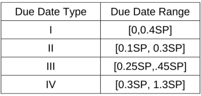
In order to evaluate the performances of the proposed heuristics, we conducted experiments on several randomly generated problems with sizes of 20, 30, 40, 60, 80, 100, 150 jobs. The processing times are taken as uniformly distributed in the range [0,25] and [0,100] representing low and high processing time variability, respectively. The due dates are also distributed uniformly on the four different ranges as shown in Table 2. Here, SP denotes the sum of processing times of the N jobs. Note that, these due date and processing time distributions are used in Keha and Koksalan (2003).

Table 2: Due Date Ranges

Due Date Type Due Date Range

I [0,0.4SP] II [0.1SP, 0.3SP] III [0.25SP,.45SP] IV [0.3SP, 1.3SP]

Before performing an extensive numerical study, we solved about 50 sample problems with 20, 30, 40 and 60 jobs to gain some insights on the significant beam width values to use in our experiments with BS-I and BS-D. For this purpose, we consider the behavior of average percentage deviation of each heuristic from optimum with respect to increasing beam widths. In this context, we define the average percentage deviation of a heuristic from optimum as

Average Percentage Deviation =

∑ ∑

∑ ∑

Here, M is the total number of problems, F (m,n) is the minimum mean flowtime resulting from the heuristic solution of the mth problem for nT = n, and

F OPT(m,n) is the corresponding optimal solution. nT(m,Moore) and nT(m,SPT) are

the number of tardy jobs in sequences formed according to Moore’s Algorithm and SPT order, respectively, for the mth problem. Finally, ϕm,n is defined as

1, if F(m,n)> F_OPT(m,n)

n m,

ϕ = 0, o.w.

Average percentage deviation illustrates the average gap between the heuristic and the optimal solution over all efficient schedules and test problems where this gap is positive. These cases will be referred to as deviation instances in the rest of the thesis. Figure 1 illustrates average percentage deviation of BS-D with respect to increasing beam width values in sample problems. As seen in Figure 1, the average percentage deviation is stabilized after a beam width value of 10. Therefore, in the rest of the experiments we use BS-I and BS-D with beam width value 10.

6.1 Comparison with the Optimal Solution

In this subsection, we report the results of our comparison of the proposed heuristics with the optimal solution considering several measures. Since Nelson’s B&B Algorithm can solve problems with size up to 60 jobs within reasonable amount of time, comparing the heuristics with optimal solution on larger size

Figure1: Average Percentage Deviation of BS-D from Optimum vs Beam Width

0 0.05 0.1 0.15 0.2 0.25 0.3 1 3 5 7 9 11 13 15 17 19 21 23 25 27 29 31 33 35 Beam Width A ver age P e rcent a ge D evi at io n

problems is not possible. Therefore we decided to solve problems with sizes of 20, 30, 40, 60 jobs. The processing time and due date values for these problems have been generated according to our discussion early in Chapter 6. For each job size, due date and processing time distribution, we solved 5 randomly generated problems.

Considering all possible combinations, we have solved 40 (2x4x5) problems for each job size which makes 160 in total. These 160 problems were solved with Nelson’s B&B method, BS-I, BS-D, Keha and Koksalan (2003)’s genetic algorithm (GA(K&K)), Koktener and Koksalan (2000)’s simulated annealing (SA(K&K)), proposed tabu-search (TS) and proposed genetic algorithm (GA). Keha and Koksalan (2003) use tournament selection method to choose two parent schedules which are modified in order to build two new schedules. Tournament selection is choosing the best schedules with respect to a fitness function as parents among a number of randomly selected schedules. This number is referred as tournament size. For our experiments we take tournament size as 5. In addition, we also solved the test problems with a heuristic suggested by Nelson et al. (1986). This heuristic is based on expanding the node with minimum flowtime at

each level of a given B&B tree of Nelson et al.’s optimum solution. We recognize that this heuristic is nothing but a special version of our proposed beam search algorithms with beam width 1. In the rest of the thesis, we refer to this heuristic as

Nelson’s Heuristic.

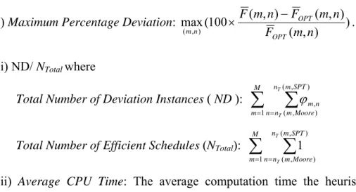
In addition to the average percentage deviation, the following three measures were considered in our experiments.

i) Maximum Percentage Deviation: ) ) , ( ) , ( ) , ( 100 ( max ) , ( _{F m n} n m F n m F OPT OPT n m − × .

ii) ND/ NTotal where

Total Number of Deviation Instances ( ND ):

∑ ∑

= = M m SPT m n Moore m n n n m T T 1 ) , ( ) , ( , ϕ

Total Number of Efficient Schedules (NTotal):

∑ ∑

= = M m SPT m n Moore m n n T T 1 ) , ( ) , ( 1

iii) Average CPU Time: The average computation time the heuristic spent in solving a test problem.

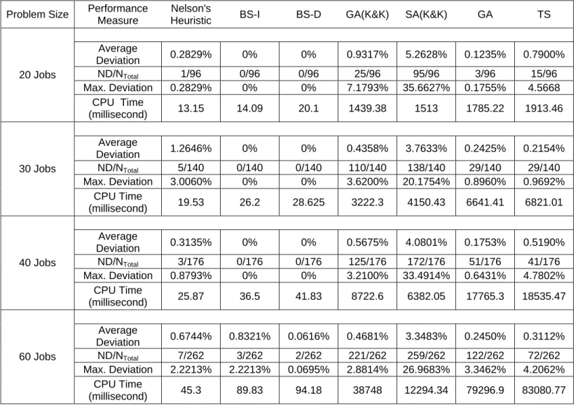
Table 3 illustrates the results of our experiments with 20, 30, 40, 60 jobs. The results indicate that both beam search based heuristics and Nelson’s Heuristic perform better than GA(K&K) and SA(K&K) according to all performance measures. Only in the 60 jobs case, the average percentage deviation value of the BS-I seems to be larger than the GA(K&K). The reason behind this is that BS-I’s average percentage deviation is calculated according to only 3 deviation instances. Since the deviation value in one of these few instances are high, average percentage deviation value of BS-I is higher than the GA(K&K). However, we conclude that both BS-I performs better than the GA(K&K) since the other performance measures favor beam search based algorithm.

Nelson’s Heuristic, BS-I and BS-D find nearly all efficient schedules optimally. As expected, both algorithms perform a bit better than the Nelson’s Heuristic since Nelson’s Heuristic is equivalent to BS-I or BS-D with beam width

1. BS-D performs slightly better than BS-I for the problems with 60 jobs. Although the performance of the GA(K&K), SA(K&K) and Nelson’s Heuristic worsens as the size of the problem increases, the performance of our proposed beam search based heuristics is quite stable with respect to problem size. Indeed, all the problems with job sizes 20, 30 and 40 were solved optimally by the proposed beam search algorithms. Only among the problems with 60 jobs, there are some instances where the F value found by BS-I and BS-D for a test problem deviate from optimum.

Both GA and TS perform better than the GA(K&K) and SA(K&K) but not as good as beam search based algorithms. GA performs a bit better than TS according to the average percentage deviation criterion. However, TS finds more efficient schedules optimally than the GA does, for the problems with 40 and 60 jobs. Their average deviation values seem to be stable according to the job size. However, as job sizes increases the rate ND/NTotal increases for both TS and GA algorithms.

Therefore, performances of these heuristics are negatively affected by the increasing problem size.

As Table 3 shows, Nelson’s Heuristic is the fastest of all 5 approximate solution methods that we tested in this experiment. Although GA(K&K)’s solution quality is better than SA(K&K)’s, GA(K&K) is much slower than SA(K&K). GA and TS are the two slowest heuristics. Indeed, Nelson’s Heuristic performs much better than these four methods resulting with less CPU time. Both of our proposed beam search algorithms work slightly slower than the Nelson’s Heuristic but faster than the others.

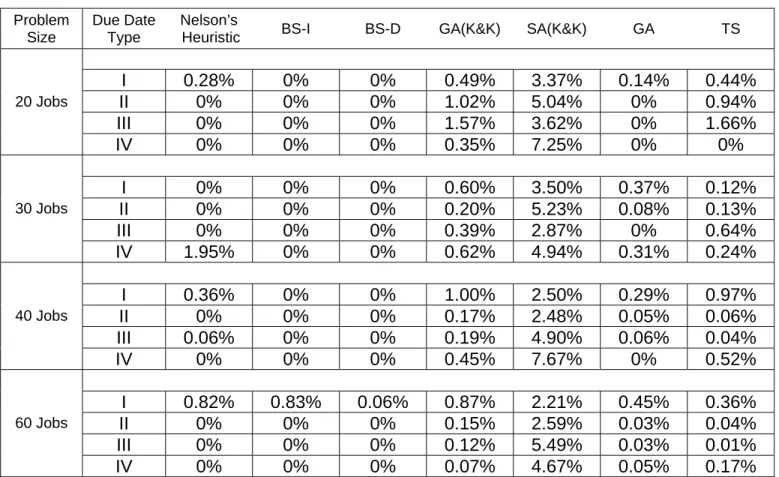
Tables 4 and 5 illustrate the average percentage deviation from optimum solution for each due date distribution type and for each problem size with low and high processing time distributions, respectively. These tables illustrate that BS-I, BS-D and Nelson’s Heuristic provide better solutions than GA, SA, SA(K&K) and

Table 3: Comparison of the Heuristics with the Optimum Solution

Problem Size Performance Measure

Nelson's

Heuristic BS-I BS-D GA(K&K) SA(K&K) GA TS Average Deviation 0.2829% 0% 0% 0.9317% 5.2628% 0.1235% 0.7900% ND/NTotal 1/96 0/96 0/96 25/96 95/96 3/96 15/96 Max. Deviation 0.2829% 0% 0% 7.1793% 35.6627% 0.1755% 4.5668 20 Jobs CPU Time (millisecond) 13.15 14.09 20.1 1439.38 1513 1785.22 1913.46 Average Deviation 1.2646% 0% 0% 0.4358% 3.7633% 0.2425% 0.2154% ND/NTotal 5/140 0/140 0/140 110/140 138/140 29/140 29/140 Max. Deviation 3.0060% 0% 0% 3.6200% 20.1754% 0.8960% 0.9692% 30 Jobs CPU Time (millisecond) 19.53 26.2 28.625 3222.3 4150.43 6641.41 6821.01 Average Deviation 0.3135% 0% 0% 0.5675% 4.0801% 0.1753% 0.5190% ND/NTotal 3/176 0/176 0/176 125/176 172/176 51/176 41/176 Max. Deviation 0.8793% 0% 0% 3.2100% 33.4914% 0.6431% 4.7802% 40 Jobs CPU Time (millisecond) 25.87 36.5 41.83 8722.6 6382.05 17765.3 18535.47 Average Deviation 0.6744% 0.8321% 0.0616% 0.4681% 3.3483% 0.2450% 0.3112% ND/NTotal 7/262 3/262 2/262 221/262 259/262 122/262 72/262 Max. Deviation 2.2213% 2.2213% 0.0695% 2.8814% 26.9683% 3.3462% 4.2062% 60 Jobs CPU Time (millisecond) 45.3 89.83 94.18 38748 12294.34 79296.9 83080.77

GA(K&K) with respect to each job size, processing time and due date distribution type. In fact, BS-I and BS-D deviate from the optimal solution only in the problems with 60 jobs, high processing times and Type 1 due dates.

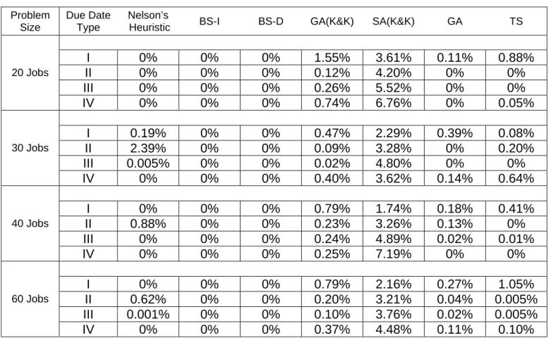
Tables 4 and 5 also indicate that the problems generated by using Type IV due date distribution are solved quite effectively by the beam search based heuristics and Nelson’s Heuristic. This distribution type represents problems with loose due dates, which implies that beam search based algorithms work well for the problems with loose due dates. Although these algorithms work also well for the problems with tighter due date distribution types (I, II, III), the most deviation instances occur in these problem types. Processing time distribution, on the other hand, does not affect the solution quality of BS-I and BS-D. For Nelson’s Heuristic, deviation from optimality mostly occurs for the problems with low processing times combined with Type 1 due dates and for problems with high processing times combined with Type 2 due dates. It can also be seen that BS-I and BS-D algorithms perform better in the problems with high processing time variability. The same situation is also valid for the GA and TS algorithms. In Appendix F, the performance measure given in Table 3 is presented for each processing time and due date distribution in detail for 20, 30, 40 and 60 jobs cases.

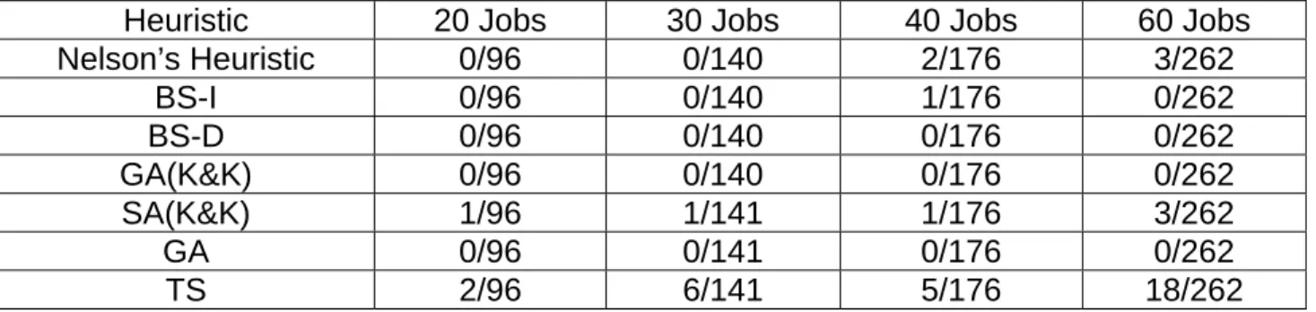
Although the quality of the solutions generated by beam search based heuristics is quite stable with respect to problem sizes, we observe that as the problem size increases Nelson’s Heuristic, BS-I, BS-D, SA(K&K) and TS algorithms may fail to find a solution for some of the efficient schedules. As stated before, for a given problem, there are nT(SPT) - nT(Moore) + 1 efficient

schedules and it is desired to find each of these schedules approximately. However, in some of the 160 test problems, beam search based heuristics, Nelson’s Heuristics, SA(K&K) and TS fail to find an approximate solution

Table 4: Average Deviation from Optimum in the Problems with Low Processing Time Variability Problem Size Due Date Type Nelson’s

Heuristic BS-I BS-D GA(K&K) SA(K&K) GA TS I 0.28% 0% 0% 0.49% 3.37% 0.14% 0.44% II 0% 0% 0% 1.02% 5.04% 0% 0.94% III 0% 0% 0% 1.57% 3.62% 0% 1.66% 20 Jobs IV 0% 0% 0% 0.35% 7.25% 0% 0% I 0% 0% 0% 0.60% 3.50% 0.37% 0.12% II 0% 0% 0% 0.20% 5.23% 0.08% 0.13% III 0% 0% 0% 0.39% 2.87% 0% 0.64% 30 Jobs IV 1.95% 0% 0% 0.62% 4.94% 0.31% 0.24% I 0.36% 0% 0% 1.00% 2.50% 0.29% 0.97% II 0% 0% 0% 0.17% 2.48% 0.05% 0.06% III 0.06% 0% 0% 0.19% 4.90% 0.06% 0.04% 40 Jobs IV 0% 0% 0% 0.45% 7.67% 0% 0.52% I 0.82% 0.83% 0.06% 0.87% 2.21% 0.45% 0.36% II 0% 0% 0% 0.15% 2.59% 0.03% 0.04% III 0% 0% 0% 0.12% 5.49% 0.03% 0.01% 60 Jobs IV 0% 0% 0% 0.07% 4.67% 0.05% 0.17%

Table 5: Average Deviation from Optimum in the Problems with High Processing Time Variability Problem Size Due Date Type Nelson’s

Heuristic BS-I BS-D GA(K&K) SA(K&K) GA TS I 0% 0% 0% 1.55% 3.61% 0.11% 0.88% II 0% 0% 0% 0.12% 4.20% 0% 0% III 0% 0% 0% 0.26% 5.52% 0% 0% 20 Jobs IV 0% 0% 0% 0.74% 6.76% 0% 0.05% I 0.19% 0% 0% 0.47% 2.29% 0.39% 0.08% II 2.39% 0% 0% 0.09% 3.28% 0% 0.20% III 0.005% 0% 0% 0.02% 4.80% 0% 0% 30 Jobs IV 0% 0% 0% 0.40% 3.62% 0.14% 0.64% I 0% 0% 0% 0.79% 1.74% 0.18% 0.41% II 0.88% 0% 0% 0.23% 3.26% 0.13% 0% III 0% 0% 0% 0.24% 4.89% 0.02% 0.01% 40 Jobs IV 0% 0% 0% 0.25% 7.19% 0% 0% I 0% 0% 0% 0.79% 2.16% 0.27% 1.05% II 0.62% 0% 0% 0.20% 3.21% 0.04% 0.005% III 0.001% 0% 0% 0.10% 3.76% 0.02% 0.005% 60 Jobs IV 0% 0% 0% 0.37% 4.48% 0.11% 0.10%

specifically for the efficient schedule that have nT(Moore) tardy jobs (Table 6).

The number of the problems such a situation occurs is relatively small, and most of the cases that can not be solved by Nelson’s Heuristic, are solved by BS-I and BS-D. Nevertheless, the number of these instances seems to be increasing as the problem size increases. In order to see whether this trend will continue for larger problem sizes and to better observe the performance of our heuristics, we performed some further experiments on problems with 80,100 and150 jobs.

Table 6: Number of Efficient Schedules for which No Solution is Found

Heuristic 20 Jobs 30 Jobs 40 Jobs 60 Jobs Nelson’s Heuristic 0/96 0/140 2/176 3/262 BS-I 0/96 0/140 1/176 0/262 BS-D 0/96 0/140 0/176 0/262 GA(K&K) 0/96 0/140 0/176 0/262 SA(K&K) 1/96 1/141 1/176 3/262 GA 0/96 0/141 0/176 0/262 TS 2/96 6/141 5/176 18/262

6.2 Experiments on Larger Problems

We generated larger size problems with 80, 100 and 150 jobs using the same processing time and due date distributions stated before. For each job size, processing time and due date distribution type, we generated 5 problems and obtained 120 problems in total. We compared Nelson’s Heuristic with I, BS-D, GA, TS, SA(K&K) and GA(K&K) algorithms and measured their relative performance. In our experiments with larger problems, we first consider average percentage difference of each heuristic’s solution from Nelson’s Heuristic. The average percentage difference is the arithmetic mean of the percentage differences

over all the efficient solutions and all the problems with the same size. In mathematical terms, it is defined as follows.

Average Percentage Difference =

∑ ∑

∑ ∑

where F (m,n) is the minimum flowtime provided by the considered heuristic for the mth problem when nT = n. FNelson(m,n) is the minimum flowtime resulting

from Nelson’s Heuristic. nT(m,Moore) and nT(m,SPT) are the number of tardy jobs

in the sequences formed according to Moore’s Algorithm and SPT order, respectively, for the mth problem. Finally, ψ_m,n is given below.

1, if F(m,n)≠ FNelson(m,n)

n m,

ψ = 0, o.w.

The other measures we consider in the experiments with larger problems are as follows.

N+: Number of cases where a specific heuristic performs better than the Nelson’s

Heuristic. N+ =

∑ ∑

N-: Number of cases a specific heuristic performs worse than the Nelson’s

Heuristic. N- =

∑ ∑

1, if F(m,n)< F_Nelson(m,n)

n m,

μ = 0, o.w.

Maximum Percentage Difference: ) ) , ( ) , ( ) , ( 100 ( max ) , ( _{F m n} n m F n m F Nelson Nelson n m − × .

Minimum Percentage Difference: ) ) , ( ) , ( ) , ( 100 ( min ) , ( _{F m n} n m F n m F Nelson Nelson n m − × .

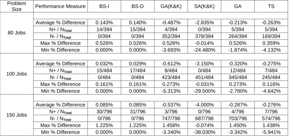
The corresponding results are presented in Table 7. As seen in the table, proposed heuristics and Nelson’s Heuristic perform better than the SA(K&K), GA(K&K), GA and TS, also in larger size problems with respect to all these measures. As it can be understood from the N+/NTotal measure, in more than %90

of the cases Nelson’s Heuristic performs better than or equal to these iterative algorithms.

Proposed beam search algorithms perform slightly better than the Nelson’s Heuristic. As the job size increases, number of instances in which proposed heuristics perform better than the Nelson’s Heuristic increases. We also observe that BS-D performs slightly better than the BS-I on the problems with larger job sizes. In most of the cases, however, their solution qualities are almost the same. As it can be seen in Table 7, BS-D outperforms Nelson’s Heuristic in a few more instances than BS-I does.GA and TS perform better than the GA(K&K) and SA(K&K) almost for all measures presented in Table 7. TS and GA’s performance are nearly same for the cases in which they both find a solution. In

Table 7: Comparison of the other Heuristics with Nelson’s Heuristic Problem

Size Performance Measure BS-I BS-D GA(K&K) SA(K&K) GA TS Average % Difference 0.143% 0.140% -0.487% -2.835% -0.213% -0.263% N+ / NTotal 14/394 15/394 4/394 0/394 5/394 5/394 N- / NTotal 0/394 0/394 352/394 378/394 264/394 169/394 Max % Difference 0.526% 0.526% 0.526% -0.014% 0.526% 0.359% 80 Jobs Min % Difference 0.000% 0.000% -3.693% -24.480% -1.874% -4.132% Average % Difference 0.032% 0.029% -0.612% -3.150% -0.320% -0.275% N+ / NTotal 15/484 17/484 8/484 0/484 12/484 7/484 N- / NTotal 0/484 0/484 423/484 451/484 345/484 245/484 Max % Difference 0.161% 0.161% 0.273% -0.031% 0.273% 0.116% 100 Jobs Min % Difference 0.000% 0.000% -5.313% -29.500% -2.780% -4.642% Average % Difference 0.085% 0.085% -0.537% -4.000% -0.287% -0.276% N+ / NTotal 30/796 31/796 3/796 0/796 4/796 7/796 N- / NTotal 0/796 0/796 747/796 687/796 703/796 574/796 Max % Difference 1.225% 1.225% 1.458% -0.074% 1.450% 1.438% 150 Jobs Min % Difference 0.000% 0.000% -3.340% -38.030% -3.342% -5.941%

these cases, overall average difference from Nelson’s Heuristic is nearly same. GA’s maximum deviation values are less than TS’s, and number of instances that TS performs as well as Nelson’s Heuristic is more than those that GA does. However, the real handicap of TS is that there are considerable number of instances in which it can not find an approximately efficient schedule for some NT

values (Table 8). GA, on the other hand, finds efficient schedules approximately for every instance.

In Appendix G, the performance measure given in Table 7 is presented for each processing time and due date distribution in detail for the 80, 100 and 150 jobs cases. According to the tables in Appendix G, most of the instances in which BS-I and BS-D perform better than the Nelson’s Heuristic occur among the test problems with Type I due date. These problems also require much more CPU time than the others. In addition, GA performs better than the TS in the problems with Type I and IV due date distributions and TS performs better in the problems with Type II and III due date distributions.

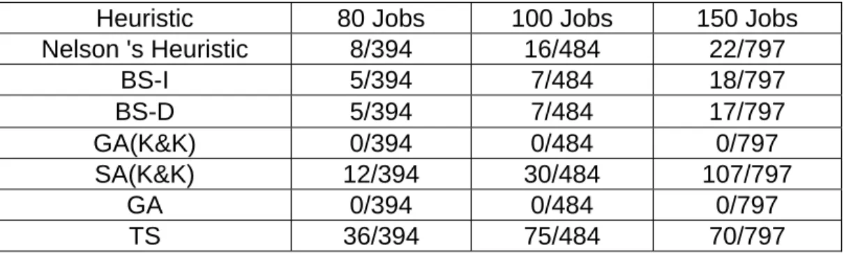
We again observed the cases where compared heuristics fail to find approximately efficient schedules for some of the NT values in the efficient range.

The number of such instances is given in Table 8. This table illustrates that as the size of the problem increases such cases appear more frequently for Nelson’s Heuristic. Problems, where feasible solutions cannot be found, frequently coincide with Type I due date distribution, and less frequently with Type II and III. BS-D and BS-I algorithms halved the number of these cases in the problems with 80 and 100 jobs. However, the experiments on the problems with 150 jobs demonstrate that the performance of our proposed algorithms on this issue worsens as the size of the problem increases.

Table 8: Number of Efficient Schedules for which No Solution is Found

Heuristic 80 Jobs 100 Jobs 150 Jobs Nelson 's Heuristic 8/394 16/484 22/797 BS-I 5/394 7/484 18/797 BS-D 5/394 7/484 17/797 GA(K&K) 0/394 0/484 0/797 SA(K&K) 12/394 30/484 107/797 GA 0/394 0/484 0/797 TS 36/394 75/484 70/797

While the number of no solution cases is quite high for SA(K&K) and TS algorithms, GA and GA(K&K) find an approximate solution for every NT value of

the problems considered in our experiments. Nevertheless, as it can be seen in Table 9, the computation time requirements for GA and GA(K&K) are a lot more than that of the beam search based algorithms. Therefore, for large size problems, if the decision makers desire to find approximately efficient schedules for all NT

values in the efficient range, they should first use BS-D or BS-I algorithms in order to minimize the number of instances where no solution is found. Then genetic algorithm should be used to solve the remaining instances.

Table 9: Average CPU Time in Milliseconds

Heuristic 80 Jobs 100 Jobs 150 Jobs Nelson's Heuristic 80.03 135.95 486.28 BS-I 276.13 570.7 2601.5 BS-D 258.15 565.25 2517.55 GA(K&K) 136836 26925.5 2057585.5 SA(K&K) 27836.76 48184.16 139499.3 GA 272333.6 681263.7 4094870.2 TS 272381.5 630742.8 3273617.3

C h a p t e r 7

CONCLUSION

As a result of our experiments, we concluded that BS-D and BS-I perform quite well for the multicriteria scheduling problem of minimizing average flowtime and number of tardy jobs. In most of the cases, these two algorithms find the efficient schedules optimally. Even in the cases where BS-D or BS-I deviate from optimum, the deviation is quite small and the deviation is stable with respect to problem size. In addition, both BS-D and BS-I perform better than the other heuristics given in this thesis with respect to all problem types that we test. The only disadvantage of our proposed beam search heuristics is that, they, although rarely in some cases, fail to find approximately efficient solutions for some of the nT values in the efficient ranges. For such cases, we

propose that GA or GA(K&K) be used.

We believe that the good performance of our proposed approach is due to the beam search mechanism. In fact, GA(K&K) and SA(K&K), which are two existing heuristics in the literature, search among all possible sequences for the efficient schedules. However, BS-I and BS-D limit the search space by utilizing Theorem 1 and Smith’s Algorithm. Hence, they find better solutions by searching a smaller space and more efficiently than GA(K&K) and SA(K&K) do.

Theorem 1 and Smith’s Algorithm are also utilized by GA and TS. Therefore, GA and TS outperform GA(K&K) and SA(K&K). However, our

experiments show that in general the proposed beam search algorithms perform better than GA and TS. Since, this study shows that utilizing the characteristics of the efficient solutions in the approximate or optimal solution methods to limit the search space is quite effective; we believe that such a beam search mechanism can be also quite beneficial to solve the other multicriteria scheduling problems. Therefore, we strongly suggest using this technique in the future multicriteria scheduling studies.

As further studies, BS-I and BS-D can also be applied to the other bicriteria single machine problems such as minimizing weighted flowtime and number of tardy jobs, and minimizing weighted flowtime and weighted number of tardy jobs. With the insights gained from this study, we already extended our current research to consider the first problem. We consider the second problem which seems to be more challenging, as a future work.

We believe that beam search applications are quite promising to solve multicriteria scheduling problems in general. Therefore, another line of research may extend this work to more complex settings, such as parallel machine environments. As a final open area of possible investigation, we note the robustness of the solutions which is a fundamental application issue.

BIBLIOGRAPHY

Aydogdu, M., Sabuncuoglu, I., 2006. “A Tabu-searh algorithm for the single machine bicriteria scheduling problem: Minimization of average flowtime and number of tardy jobs”. Technical Report, Bilkent University IE Department. Billaut, J.-C., T_kindt, V., 1999. “Some guidelines to solvemulticriteria scheduling problems”, IEEE International Conference on Systems, Man and

Cybernetics Proceeding. 6, 463–468.

Blum, C., 2002. “ACO applied to group shop scheduling: A case study on intensification and diversification, in M. Dorigo, G. Di Caro and M. Sampels (eds)”, Proceedings of ANTS 2002 – From Ant Colonies to Artificial Ants: Third

International Workshop on Ant Algorithms, Lecture Notes in Computer Science.

2463, 14–27.

Chen, C.L., Bulfin, R.L., 1993. “Complexity of single machine multi-criteria scheduling problems”, European Journal of Operational Research. 70, 115–125. Dileepan. P, Sen. T., 1988. “Bicriterion static scheduling research for a single machine”, Omega. 16-1, 53-59.

Duarte, R., Rego, C., Gamboa, D., 2004. “A Filter and Fan Approach for the Job Shop Scheduling Problem: A Preliminary Study”, Proceedings: International

Conference on Knowledge Engineering and Decision Support. 401-406.

Emmons, H., 1975. “One machine sequencing to minimize mean flowtime with minimum tardy”, Naval Research Logistics Quarterly. 22-3, 585-592.

Erol, S., Guner, E., Tani, K., 1998. “One machine scheduling to minimize maximum earliness with minimum number of tardy jobs”, International Journal

of Production Economics. 55, 213-219.

Fry, T., Armstrong, R., Lewis H., 1989. “A framework for single machine multiple objective scheduling research”, Omega. 17-6, 595 - 607.

Ghirardi, M., Potts, C. N., 2005. “Makespan minimization for scheduling unrelated parallel machines: A recovering beam search approach”, European

Journal of Operational Research. 165-2, 457–467.

Heck, H., Roberts, S., 1992. “A note on the extension of a result on scheduling with secondary criteria”, Naval Research Logistics Quarterly. 19, 403-405.

Hoogeveen, J.A., 2005. “Multicriteria Scheduling”, European Journal of

Operational Research. 167-3, 592-623.

Huo, Y., Leung, J. Y. T., Zhao, H., 2004. “Complexity of two-dual criteria scheduling problems”, Submitted to Operations Research Letters.

Kardas, S., Sabuncuoglu, I., 2006. “A Genetic algorithm for the single machine bicriteria scheduling problem: Minimization of average flowtime and number of tardy jobs”. Technical Report, Bilkent University IE Department.

Keha, A. B., Koksalan, M., 2003. “Using genetic algorithms for single-machine bicriteria scheduling problems”, European Journal of Operational Research. 145, 543–556.

Kiran, A. S., Unal A. T., 1991. “A single-Machine Problem with multiple Criteria”, Naval Research Logistics. 38, 721-727.

Koksalan, M., 1999. “A Heuristic Approach to Bicriteria Scheduling”, Naval

Koksalan, M., Azizoglu, M., Kondakci, S., 1998. “Minimizing flowtime and maximum earliness on a single machine”, IIE Transactions. 30, 192–200.

Koktener, E.K., Koksalan, M., 2000. “A simulated annealing approach to bicriteria scheduling problems on a single machine”, Journal of Heuristics. 6, 311–327.

Kondakci, S., Azizoglu, M., Köksalan, M., 2003. “Scheduling with multiplecriteria”, Computers & Industrial Engineering. 45-2, 257-269.

Kondakci, S. K., Bekiroglu T., 2000. ”Scheduling with bicriteria: total flowtime and number of tardy jobs”, International Journal of Production Economics. 53, 91- 99.

McMullen, P., Tarasewich, P., Frazier, G., 2000, “Using genetic algorithms to solve the multi-product JIT sequencing problem with set-ups”, International

Journal of Production Research. 38-12, 2653-2670.

Moore, J. M., 1968. “An n job, one machine sequencing algorithm for minimizing the number of late jobs”, Management Science. 15, 102-109.

Nagar, A., Haddock, J., Heragu, S., 1995. “Multiple and bicriteria scheduling: A literature survey”, European Journal of Operations Research. 81, 88 –104.

Nelson, R. T., Sarin, R. K., Daniels, R. L., 1986. “Scheduling with multiple performance measures: the one machine case”, Management. Science 32-4, 464-479.

Sabuncuoglu, I. Bayiz. M., 1999. “Job shop scheduling with beam search”,

European Journal of Operational Research. 118-2, 390-412.

Sabuncuoglu, I., Karabuk, S., 1998. “A beam search algorithm and evaluation of scheduling approaches for FMSs”, IIE Transactions. 30-2, 179-191.

Sen, T., Gupta, S. K., 1983. “A branch and bound procedure to with multiple performance measures: the one machine case”, Management Science. 32, 464-479.

Smith, W. E., 1956. “Various Optimizers for Single Stage Production”, Naval

Research Logistics Quarterly 3, 1-2.

T’kindt, V., Bouibede-Hocine, K., Esswein, C., 2005. “Counting and enumeration complexity with application to multicriteria scheduling”. A quarterly Journal of

Operations Research. 3-1, 1-21.

Wan, G., Yen, B. P. C., 2003. “Single Machine Bicriteria Sceduling: A survey”,

APPENDIX

A. Example for Nelson et al.’s (1986) Branch and Bound

Algorithm

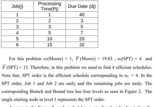
The process times and the due dates of our example are given below.

Table 1: Sample Problem Parameters Job(j) Processing

Time(Pj) Due Date (dj)

1 1 40 2 2 3 3 3 5 4 5 7 5 10 20 6 15 32

For this problem nT(Moore) = 1, F (Moore) = 19.83 , nT(SPT) = 4 and F (SPT) = 13. Therefore, in this problem we need to find 4 efficient schedules.

Note that, SPT order is the efficient schedule corresponding to nT = 4. In the

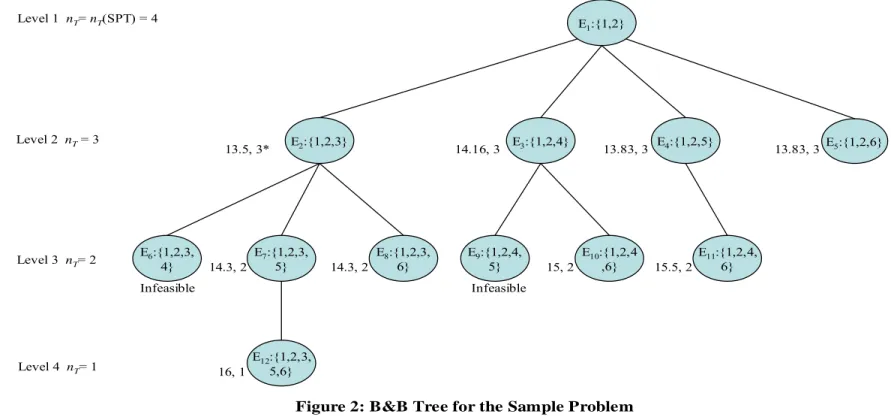
SPT order, Job 1 and Job 2 are early and the remaining jobs are tardy. The corresponding Branch and Bound tree has four levels as seen in Figure 2. The single starting node in level 1 represents the SPT order.

As seen in the Figure 2, each node k has a set of early jobs denoted as Ek.

Since the starting node at level 1 represents SPT order, E1: {1, 2} is the set of

jobs that is early in the SPT order. In the efficient schedule for nT = 3, besides

Job 1 and Job 2 another job among 3,4,5 and 6 must be also early (See Theorem 1). Thus, at the second level, these four jobs are tried one by one by

E₁:{1,2} E₂:{1,2,3} E₃:{1,2,4} E₄:{1,2,5} E₅:{1,2,6} 13.5, 3* 14.16, 3 13.83, 3 13.83, 3 E₆:{1,2,3, 4} E₇:{1,2,3, 5} E₈:{1,2,3, 6} Infeasible 14.3, 2 14.3, 2 E₁₀:{1,2,4 ,6} E₉:{1,2,4, 5} 15, 2 Infeasible E₁₁:{1,2,4, 6} 15.5, 2 E₁₂:{1,2,3, 5,6} 16, 1 Level 1 n_T= n_T(SPT) = 4 Level 2 n_T= 3 Level 3 n_T= 2 Level 4 nT= 1

Figure 2: B&B Tree for the Sample Problem

being added to the set of early jobs referred by 2nd, 3rd, 4th and 5th nodes. For example, in the 2nd node, Job 3 is added to E3, and then, by using Smith’s

Algorithm, the schedule that gives minimum flowtime while keeping jobs 1, 2 and 3 non-tardy is found. The resulting flowtime is 13.5. In a similar fashion, other three nodes at the second level are constructed, and the minimum flowtime values are found as 14.16, 13.83 and 13.83. Since the smallest flowtime at this level is given by the second node, the efficient schedule for nT = 3 corresponds to the

sequence at this node.

At the third level, all possible subsets of {3,4,5,6} (tardy jobs in SPT order) with cardinality two is added to the early jobs of SPT order to find efficient schedule for nT = 2. For this reason, each node at level 2 is further expanded by

adding one more job. For example, node 2 (E2: {1,2,3}) is expanded to the next

level to form nodes 6, 7, and 8 by adding job 4, 5 and 6. Node 3 (E3: {1,2,4}) is

expanded to the next level to form nodes 9 and 10 by adding jobs 5 and 6. However, Job 4 is not added to E3 to prevent repetition. After all nodes are

expanded to level three, for each node, Smith’s Algorithm is run. As a result, it appears that efficient schedule for nT = 2 is the one that corresponds to E7 =

{1,2,3,5} with flowtime 14.3. The algorithm continues in this manner.

B. Example for Independent Beam Search Algorithm

As an example, we consider the problem given in Appendix-A. Let us solve the same problem also with independent beam search algorithm. As can be seen in Figures 2 and 3, the first two levels of both the B&B and the BS-I tree are the same. Both trees start with a node that represents SPT order. Then, four new nodes are expanded from this initial node by adding jobs 3,4,5 and 6 to E2, E3, E4 and E5,

respectively. Using Smith’s Algorithm, the schedules that give minimum flowtime while keeping the jobs in E2, E3, E4 and E5 nontardy are found. Since the schedules

found for nodes 2 and 4 have the smallest flowtime, they are selected to be expanded to the next level.

At level 3, the new nodes are generated by adding one more job to E2 and E4.

Nodes 6, 7 and 8 are generated by adding jobs 4, 5 and 6 to E2. Similarly, nodes 9,

10 and 11 are generated by adding jobs 3, 4 and 6 to E4. As the schedules found

for nodes 7 and 9 have the smallest F values, they are expanded to the next level. The algorithm continues in a similar way for the fourth level.

E₁:{1,2} E2:{1,2,3} E3:{1,2,4} E4:{1,2,5} E5:{1,2,6} 13.5, 3 14.16, 3 13.83, 3 13.83, 3 E6:{1,2,3, 4} E7:{1,2,3, 5} E8:{1,2,3, 6} Infeasible 14.3, 2 14.3, 2 E10:{1,2,5, 4} E11:{1,2,5, 6} 15.5, 2 E13:{1,2,3 5,6} 16, 1 Level 1 nT= nT(SPT) = 4 Level 2 n_T= 3 Level 3 n_T= 2 Level 4 nT= 1

Figure 3: Independent Beam Search Tree for the Sample Problem where b = 2

E9:{1,2,5, 3} 14.3, 2 E12:{1,2,3 5,4} E15:{1,2,5 3,6} E14:{1,2,5 3,4} 16, 1 Infeasible Infeasible Infeasible

C. Example for Dependent Beam Search Algorithm

Dependent beam search algorithm is also applied to the sample problem given in Appendix-A. The results are presented in Figure 4. As can be seen in Figure 4, at the third level, the two nodes with minimum F value are nodes 7 and 8. Without considering the fact that both these nodes are expanded from the node 2, they are expanded to the next level.

E1:{1,2} E₂:{1,2,3} E₃:{1,2,4} E₄:{1,2,5} E₅:{1,2,6} 13.5, 3 14.16, 3 13.83, 3 13.83, 3 E6:{1,2,3 4} E7:{1,2,3 5} E8:{1,2,3 6} Infeasible 14.3, 2 14.3, 2 E10:{1,2,5 4} E11:{1,2,5 6} 15.5, 2 E₁₃:{1,2,3 5,6} 16, 1 Level 1 n_T= n_T(SPT) = 4 Level 2 n_T= 3 Level 3 n_T= 2 Level 4 n_T= 1

Figure 4: Dependent Beam Search Tree for the Sample Problem where b = 2

E9:{1,2,5 3} 14.3, 2 E₁₂:{1,2,3 5,4} E₁₅:{1,2,3 6,5} E₁₄:{1,2,3, 6,4} 16, 1 Infeasible Infeasible Infeasible